Floating Black Hole in the Karch-Randall Model
and its Holographic Dual

Abstract:

To investigate the holography in the Karch-Randall (KR) braneworld model, we construct time-symmetric initial data of black holes floating in the bulk, and compare it with its holographic dual, which is described by four-dimensional self-gravitating quantum field theory in asymptotically AdS₄ spacetime. We also give a definition and an explicit formula of mass in the KR model extending the definition by Abbott and Deser for asymptotically AdS spacetime. We obtain supporting evidence for the holography in the KR model such as good agreements of phase structures and characteristic values between the two theories, and find clues that the Hawking-Page transition of the four-dimensional quantum theory in a microcanonical ensemble is holographically dual to a transition in the bulk black hole configuration.

1 Introduction

The AdS/CFT correspondence [1] has been attracting intensive attentions these years, and its extensions are discussed in wide settings. In this paper, we focus on one of such an extension to the braneworld models. The Randall-Sundrum (RS) model [2] is a braneworld model that is composed of infinitely extending AdS₅ bulk and a four-dimensional positive tension brane. A remarkable feature of this model is that four-dimensional gravity is well reproduced on the brane though the bulk spacetime is infinitely extending. If we apply the AdS/CFT correspondence to the AdS bulk, we obtain a duality of new type as follows [3, 4, 5, 6]. Since the AdS boundary is cut off by the brane in this model, we may consider the CFT resides on the brane instead of the AdS boundary. It is believed that this CFT suffers an exotic UV cutoff by this introduction of the brane. Adding to that, this deformed CFT couples to four-dimensional gravity on the brane in this setting. Though this duality is not fully established, there are many pieces of circumstantial evidence for it and still attracting much interest [7, 8, 9, 10, 11, 12, 13, 14, 15, 16].

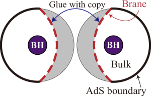
Figure 1: Schematic picture of the KR model, which is composed of $Z_{2}$-symmetric AdS₅ bulk regions and an AdS₄ brane. We consider bulk black holes in this model.

An interesting extension of this duality is to modify the four-dimensional geometry on the brane from asymptotically flat to AdS. This braneworld model with an asymptotically AdS brane is called Karch-Randall (KR) model [18], and its realization in the string theory is given in Ref. [19]. It is known that four-dimensional gravity is realized for length scale shorter than $k^{2}/\tilde{k}^{3}$, where $\tilde{k}$ and $k$ are curvatures of the brane and the bulk respectively, though there are no normalizable zero mode and four-dimensional graviton is massive. This massive graviton appears also in the four-dimensional gravity coupled to CFT due to loop correction to the graviton propagator [20, 21], so the duality seems to hold even in this extended setting. In the KR model, boundary of the bulk is a composite of the brane and the AdS boundary which share a common $S^{2}$ boundary, as is shown in Fig. 1. Then, the duality suggests that the bulk classical gravity corresponds to CFTs on those two boundaries. Since the two boundaries can communicate via bulk in the five-dimensional perspective, the CFTs on the boundaries are suggested to communicate with each other through the common boundary [22].

In the holography of this type, the CFTs couple to gravity and it is in asymptotically AdS spacetime. Then, the Hawking-Page transition may happen on the brane between thermal AdS phase and quantum-corrected black hole phase if the duality holds even in the presence of strong gravity. Based on this idea, it is conjectured that the transition in the five dimensions is realized as a configurational transition between a black hole floating in the bulk and the one localized on the brane [23]. A rough reasoning for it is as follows. When the bulk black hole is sufficiently small, it can be trapped at the throat, at which the gravitational potential is minimized. This floating black hole will induce a localized effective energy density on the brane, which can be regarded as a star made of the CFT in hydrostatic equilibrium. As we increase the bulk black hole size, it will touch the brane and become a brane-localized black hole. An observer on the brane will regard this phenomenon as a transition from a CFT star to a quantum-corrected black hole [23, 24]. In this paper, we would like to test this conjecture by constructing explicit solutions in the four-dimensional and five-dimensional pictures.

However, there are some problems to conduct comparison between the four-dimensional CFT stars and five-dimensional bulk black holes. Since the CFT stars are static objects, we should compare them with static solutions in five-dimensions, though we do not know such a static solutions so far. Another problem is that we do not know much about self-gravitating CFT. We cope with these difficulties by some approximations. Firstly, we use five-dimensional time-symmetric initial data, which is a snapshot of a momentarily static spacetime, instead of static solutions. This initial data will share some common properties with static solutions, especially when its mass is minimized among the available set of initial data with the same entropy. If the initial data set is complete, that initial data with minimum mass will be a static solution. Next, we use radiation fluid approximation of the four-dimensional self-gravitating CFT, which is valid for high enough temperature [24, 26]. We later see that this condition of high temperature is always satisfied in the regime we are interested in. Using these approximations, we construct solutions numerically in four-dimensional and five-dimensional picture and test the conjecture of duality. As a first step, we focus on the bulk floating black holes and the four-dimensional CFT stars, and study the duality between them.

One problem in the analysis is that there is no known good definition of mass so far in the KR model, which is necessary to know the thermodynamic properties of the five-dimensional system. In this paper, we give an appropriate definition of mass in the KR model according to Abbott and Deser’s definition of mass in an asymptotically AdS spacetime [27]. This is another feature of this work.

Organization of this paper is as follows. We firstly illustrate how to construct a floating black hole initial data in Sec. 2. In Sec. 3, we propose a definition of mass in the KR model and give an explicit mass formula for initial data constructed in Sec. 2. Using these tools, we analyze the initial data and summarize their basic properties in Sec 4. After that, we compare the five-dimensional bulk floating black holes with four-dimensional CFT stars in Sec. 5. We briefly summarize how to construct CFT star solutions, and then we compare them with the initial data. We find good agreements of phase structures and characteristic values between them. Finally, we give concluding remarks in Sec. 6.

2 Floating black hole initial data

In this section, we illustrate the construction method of time-symmetric initial data of floating black holes in the KR model. An initial data is a set of spatial geometry and its time derivatives which solves the Hamiltonian constraint and momentum constraints in the Einstein equations. In the case that the spacetime is time-symmetric about a $t=\text{constant}$ surface, the momentum constraints are trivially satisfied. Thus we have to solve only the Hamiltonian constraint in this case.

To construct an initial data of the KR model, we have to solve the five-dimensional Hamiltonian constraint in the bulk and the four-dimensional one on the brane simultaneously. In this work, we solve those equations by taking a well-known static solution in the bulk and embedding the brane that satisfies the constraints.

In the bulk, we take the AdS-Schwarzschild solution:

$$ds^{2}=-Udt^{2}+\frac{dr^{2}}{U}+r^{2}\left(d\chi^{2}+\sin^{2}\chi\,d\Omega_{\text{II}}\right)~{}~{},\qquad U=1+k^{2}r^{2}-\frac{\mu}{r^{2}}~{}~{},$$ (1)

where $k$ is the five-dimensional bulk curvature, which is related to the five-dimensional cosmological constant as $\Lambda_{\text{5}}=-6k^{2}$. $\mu$ is the mass parameter of the black hole, and $d\Omega_{\text{II}}$ is the metric of a unit two-sphere. The black hole horizon is at $r_{g}$, the largest root of the equation $U(r)=0$.

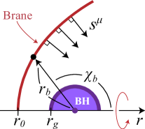
Figure 2: Configuration of the brane and the black hole in an initial data in the global coordinates.

Taking this AdS-Schwarzschild black hole spacetime as a background, we determine the brane trajectory on it solving the four-dimensional Hamiltonian constraint. Let us introduce four-dimensional induced metric on the brane $\gamma_{ab}$ and unit normal of the brane $s_{\mu}$ that extends from the brane into the bulk. Here the Latin indices ($a,b,\dots$) run through only the four-dimensional coordinates parallel to the brane. The extrinsic curvature of the brane is defined to be $K_{ab}=-\gamma_{a}{}^{\mu}\gamma_{b}{}^{\nu}\nabla_{\mu}s_{\nu}$.

In the KR model, the five-dimensional energy-momentum tensor along the brane $T_{ab}$ is given by

$$T_{ab}=\sigma\gamma_{ab}~{}~{},\qquad\sigma\equiv\frac{3\sqrt{k^{2}-\tilde{k}^{2}}}{4\pi G_{5}}~{}~{},$$ (2)

and is localized on a four-dimensional surface in the bulk. $\sigma$ is the brane tension and $\tilde{k}$ is the four-dimensional curvature that is related to the four-dimensional cosmological constant as $\Lambda_{\text{4}}=-3\tilde{k}^{2}$, and $G_{5}$ is the five-dimensional gravitational constant. This model reduces to the RS model with a flat brane by setting $\tilde{k}=0$. In this work, we focus on the regime that $k\gg\tilde{k}$, i.e. the deformation from the RS model is small.

Using these quantities, Israel’s junction conditions at the brane are written as

$$K_{ab}-K\gamma_{ab}=\frac{1}{2}\cdot 8\pi G_{5}T_{ab}~{}~{},$$ (3)

where we used the $Z_{2}$-symmetry about the brane. These equations are the five-dimensional Einstein equations integrated across the brane, and their time-time and time-space components are the Hamiltonian constraint and the momentum constraints, respectively. Let us assume here the time-symmetry about the $t=\text{constant}$ surface we are focusing on. Then, the momentum constraints are trivially satisfied, and we only have to solve the Hamiltonian constraint, which can be rewritten as

$$D_{i}s^{i}=-3\sqrt{k^{2}-\tilde{k}^{2}}~{}~{},$$ (4)

where $D$ is the covariant derivative with respect to $\gamma_{ab}$ and the index $i$ runs through only the three-dimensional spatial coordinates on the brane.

If we assume the $O(3)$ symmetry of the brane, its trajectory in the bulk can be parametrized as $(r,\chi)=\left(r_{b}(R),\chi_{b}(R)\right)$, where $R$ is the proper length along the brane measured from the axis of the $O(3)$ rotational symmetry. Under this parametrization the Hamiltonian constraint (4) becomes a set of second order differential equations about $r_{b}$ and $\chi_{b}$. Supplying the regularity condition on the axis, those equations can readily be integrated. Once the brane trajectory is determined, an initial data is obtained by cutting the bulk spacetime along the brane, taking the part of the bulk that contains the black hole, and gluing that bulk with its copy along the brane. The resultant initial data possesses two copies of bulk regions separated by a four-dimensional asymptotically AdS brane, and each bulk region encompasses a floating black hole.

In the above construction procedure, we can set freely the mass parameter $\mu$ of the background AdS-Schwarzschild spacetime and the brane’s starting point $r_{b}(0)\equiv r_{0}$. Thus, the initial data constructed by the above method constitute a two-parameter family. By the way, if we make the brane starting point $r_{0}$ too close to the bulk black hole, the brane trajectory directly falls into the black hole and an asymptotically AdS brane is not realized. Examining Eq. (4), we find the lower bound on $r_{0}$, $r_{\text{min}}$, to realize an asymptotically AdS brane to be the largest root of the equation $U(r_{\text{min}})=r_{\text{min}}^{2}(k^{2}-\tilde{k}^{2})$.

In some initial data, typically that with small $\mu$ and $r_{0}$, an apparent horizon appears that encloses the bulk black hole and crosses perpendicularly the brane. Apparent horizon appearance implies the existence of an event horizon outside of it. The black holes in such initial data are not floating in the bulk but are localized on the brane. We neglect such initial data and focus only on those with floating black holes in this work.

Before closing this section, let us summarize the series solution of the brane trajectory in the asymptotic region for the later use. The brane trajectory can be parametrized as $\chi=\chi_{b}(r)$. Expanding this expression in the asymptotic region as

$$\chi_{b}(r)=\sum_{i=0}\chi_{i}(kr)^{-i}$$ (5)

and substituting it into the Hamiltonian constraint (4), we find that $\chi_{0}$ is a free parameter and $\chi_{1}$ is determined by $k$ and $\tilde{k}$ as $\chi_{1}=\{(k/\tilde{k})^{2}-1\}^{1/2}$. The coefficients $\chi_{2}$ and $\chi_{3}$ are functions of $\chi_{0}$ and $\chi_{1}$. The equation for $\chi_{4}$ is automatically satisfied, and the remaining coefficients $\chi_{i>4}$ are determined by $\chi_{0}$ and $\chi_{4}$. Thus, the series solution in the asymptotic region constitutes a two-parameter family whose free parameters are $\chi_{0}$ and $\chi_{4}$. We see later that we can freely change the parameter $\chi_{0}$ by the Lorentz transformation, and that $\chi_{4}$ is related to the mass contained in the initial data.

3 The Abbott-Deser mass of initial data

To analyze the thermodynamic property of black holes in the KR model, we have to know about its mass. However, there is no known definition of mass in the KR model so far and it is non-trivial how to define it. In this section, we show that we can define conserved mass by generalizing the definition of mass in asymptotically AdS spacetime by Abbott and Deser. We also illustrate in detail how to calculate this Abbott-Deser mass of initial data constructed in Sec. 2. The Abbott-Deser mass we derive in Sec. 3.1 is given by a surface integral of metric perturbation in the coordinates that are Gaussian normal (GN) near the brane. We refer to it simply as GN coordinates. Since the initial data is constructed in the AdS global coordinates, we have to transform the coordinates into the GN coordinates to calculate the mass. We summarize the coordinate transformation procedure in Sec. 3.2, and study the metric perturbation due to the bulk black hole in Sec. 3.3. Finally, we give an explicit formula of the Abbott-Deser mass of the initial data in Sec. 3.4.

3.1 The Abbott-Deser mass in the KR model

In this section, we give a definition of mass in the KR model extending the definition by Abbott and Deser for asymptotically AdS spacetime. A naive extension results in an apparent violation of the mass conservation law due to the brane’s contribution. We show that this problem can be circumvented at least if we introduce the GN coordinates with respect to the brane, and that conserved mass can be appropriately defined.

The five-dimensional Einstein equations in the KR model are given by

$$G_{\mu\nu}\equiv R_{\mu\nu}-\frac{1}{2}Rg_{\mu\nu}+\Lambda_{\text{5}}g_{\mu\nu}+\frac{\sigma\delta(y-y_{b})}{\sqrt{g_{yy}}}\gamma_{\mu\nu}=0~{}~{},$$ (6)

where the last term is the contribution of the brane. The coordinate $y$ in the delta function is the one perpendicular to the brane in the GN coordinates in which the brane is at $y=\text{constant}$ surface at $y=y_{b}$ and the metric is taken to be $g_{y\mu}=0$ for $\nu\neq y$ on the brane.

Let us consider a background solution $\bar{g}_{\mu\nu}$ and a perturbed solution $g_{\mu\nu}$ given by $g_{\mu\nu}={\bar{g}}_{\mu\nu}+h_{\mu\nu}$. We assume that both ${\bar{g}}_{\mu\nu}$ and $g_{\mu\nu}$ solve the Einstein equations (6), and that ${\bar{g}}_{\mu\nu}$ is static and possesses a timelike Killing vector $\bar{\xi}^{\mu}$. We define $\delta G_{\mu\nu}$ to be $\mathcal{O}(h)$ part of the Einstein tensor. Then, this $\delta G_{\mu\nu}$ satisfies the first order Bianchi identity $\delta G_{\mu\nu}{}^{;\nu}=0$, where the semicolon is the background covariant derivative with respect to $\bar{g}_{\mu\nu}$, by virtue of the Einstein equations for ${\bar{g}}_{\mu\nu}$.

Using these equations, conserved energy can be defined as follows. Firstly, $\delta G_{\mu\nu}$ can be rewritten as

$$\delta G_{\mu\nu}= \phantom{+}K_{\mu\alpha\nu\beta}{}^{;\beta\alpha}+\frac{1}{2}\left(\bar{R}_{\nu\rho}H^{\rho}{}_{\mu}+\bar{R}_{\lambda\nu\mu}{}^{\rho}H^{\lambda}{}_{\rho}\right)$$

$$+\frac{1}{2}h^{\lambda\rho}\bar{R}_{\lambda\rho}g_{\mu\nu}-\frac{1}{2}\bar{R}h_{\mu\nu}+\Lambda h_{\mu\nu}+\delta\left\{\frac{\sigma\delta(y-y_{b})}{\sqrt{g_{yy}}}\gamma_{\mu\nu}\right\},$$ (7)

where the $K_{\mu\alpha\nu\beta}$ and $H_{\mu\nu}$ are defined as

$$K_{\mu\alpha\nu\beta}\equiv\frac{1}{2}\left(\bar{g}_{\mu\beta}H_{\nu\alpha}+\bar{g}_{\nu\alpha}H_{\mu\beta}-\bar{g}_{\mu\nu}H_{\alpha\beta}-\bar{g}_{\alpha\beta}H_{\mu\nu}\right)~{},\qquad H_{\mu\nu}\equiv h_{\mu\nu}-\frac{1}{2}h\bar{g}_{\mu\nu}~{},$$ (8)

and indices are raised by the background metric ${\bar{g}}_{\mu\nu}$. $\delta\left\{\sigma\delta(y-y_{b})\gamma_{\mu\nu}/\sqrt{g_{yy}}\right\}$ is $\mathcal{O}(h)$ part of $\sigma\delta(y-y_{b})\gamma_{\mu\nu}/\sqrt{g_{yy}}$. Contracting Eq. (7) with $\bar{\xi}^{\mu}$ and using the background Einstein equations ${\bar{G}}_{\mu\nu}=0$, we obtain

$$\delta G_{\mu\nu}\bar{\xi}^{\nu}= \left(K_{\mu\alpha\nu\beta}{}^{;\beta}\bar{\xi}^{\nu}-K_{\mu\beta\nu\alpha}\bar{\xi}^{\nu;\beta}\right)^{;\alpha}$$

$$+\frac{\sigma\delta(y-y_{b})}{2\sqrt{\bar{g}_{yy}}}\left(-2\bar{\gamma}^{\lambda\nu}h_{\mu\nu}\bar{\xi}_{\lambda}+h\bar{\gamma}_{\mu}{}^{\lambda}\bar{\xi}_{\lambda}-\bar{\gamma}_{\rho\lambda}h^{\rho\lambda}\bar{\xi}_{\mu}\right)+\delta\left\{\frac{\sigma\delta(y-y_{b})}{\sqrt{g_{yy}}}\gamma_{\mu\nu}\right\}\bar{\xi}^{\nu}~{}.$$ (9)

Then, we define the Abbott-Deser mass $M$ as

$$M\equiv\frac{1}{8\pi G_{5}}\int_{\Sigma}d^{4}x\sqrt{-{\bar{g}}}\;\delta G^{\tau\nu}\bar{\xi}_{\nu}~{}~{},$$ (10)

where $\tau$ is the time coordinate of the GN coordinates, and the integral is taken over a large four-dimensional volume $\Sigma$. When there are no brane, i.e. $\sigma=0$, Eq. (9) becomes a total divergence, and we can transform Eq. (10) into a surface integral over three-dimensional spacelike surface $\partial\Sigma$. It implies the conservation of $M$.

We show below that this conservation law holds even when the brane exists, at least in the GN coordinates. In our setting, the background spacetime including the brane is assumed to be static and the coordinates are taken to be in the GN coordinates, i.e. $\bar{\xi}^{\mu}=0=\bar{\gamma}_{0\mu}$ for $\mu\neq t$ and $\bar{g}_{y\mu}=0$ for $\mu\neq y$. Then, the terms in Eq. (9) other than the total divergence term reduce to

$$\frac{\sigma\delta(y-y_{b})}{2\sqrt{\bar{g}_{yy}}}\!\left(-2\bar{\gamma}^{\tau\nu}h_{\tau\nu}+h-\bar{\gamma}_{\rho\sigma}h^{\rho\sigma}\right)\!\bar{\xi}_{\tau}+\delta\left\{\frac{\sigma\delta(y-y_{b})}{\sqrt{g_{yy}}}\gamma_{\tau\tau}\right\}\!\bar{\xi}^{\tau}\\ =\frac{\sigma\delta(y-y_{b})}{2\sqrt{\bar{g}_{yy}}}\left(-2h^{\tau}_{~{}\tau}+h^{y}_{~{}y}\right)\bar{\xi}_{\tau}+\delta\left\{\frac{\sigma\delta(y-y_{b})}{\sqrt{g_{yy}}}\gamma_{\tau\tau}\right\}\bar{\xi}^{\tau}~{}.$$ (11)

Let us assume here that the perturbed metric $g_{\mu\nu}$ is written in the GN coordinates, i.e. $h_{y\mu}=0$ for $\mu\neq y$. Under this condition, the second term in the right-hand side of Eq. (11) becomes $\sigma\delta(y-y_{b})(h^{\tau}_{~{}\tau}-h^{y}_{~{}y}/2)\bar{\xi}_{\tau}$ , and it cancels the first term. Then, the Abbott-Deser mass (10) becomes a surface integral as

$$M =\frac{1}{8\pi G_{5}}\int_{\Sigma}d^{4}x\sqrt{-{\bar{g}}}\left(K^{\tau\alpha\nu\beta}{}_{;\beta}\bar{\xi}_{\nu}-K^{\tau\beta\nu\alpha}\bar{\xi}_{\nu;\beta}\right)_{;\alpha}$$

$$=\frac{1}{8\pi G_{5}}\oint_{\partial\Sigma}dS_{\alpha}\sqrt{-\bar{g}}\left[K^{\tau\alpha\nu\beta}{}_{;\beta}\bar{\xi}_{\nu}-K^{\tau\beta\nu\alpha}\bar{\xi}_{\nu;\beta}\right]~{}~{},$$ (12)

and thus it is conserved. A proof of the Abbott-Deser mass conservation in a general coordinate system is probably possible, but we do not investigate it here.

3.2 Coordinate transformation of the background geometry

The goal of the following subsections is to calculate the Abbott-Deser mass of the initial data we constructed. The expression of the Abbott-Deser mass we defined is given in terms of the metric perturbation in the GN coordinates, while the initial data is constructed in the AdS global coordinates (1). Thus, we have to transform the coordinates first for the mass calculation. We consider the transformation of the background spacetime with no bulk black hole in this subsection, and after that we take into account the geometry deformation due to the bulk black hole in the next subsection.

When there is no bulk black hole, the metric of the KR model in the GN coordinates is given by

$$ds^{2}=dy^{2}+\frac{\tilde{k}^{2}}{k^{2}}\cosh^{2}\left(ky\right)\left(-\tilde{U}d\tau^{2}+\frac{1}{\tilde{U}}d\lambda^{2}+\lambda^{2}d\Omega_{\text{II}}\right)~{},\qquad\tilde{U}=1+\tilde{k}^{2}\lambda^{2}~{}~{},$$ (13)

where the brane location is determined by $(\tilde{k}/k)\cosh(ky_{b})=1$ . We can find the coordinate transformation from the global coordinates (1) to these GN coordinates (13) by comparing the metric components, which is summarized as

$$kr\cos\chi=\sinh\left(ky\right)~{},\quad kr\sin\chi=\tilde{k}\lambda\cosh\left(ky\right)~{},\quad U=\tilde{U}\cosh^{2}\left(ky\right)~{},\quad kt=\tilde{k}\tau~{}.$$ (14)

By this transformation, the brane trajectory in the GN coordinates is mapped to that in the global coordinates whose asymptotic behavior for $r\to\infty$ is given by $\chi_{0}=\pi/2$, as we can see from the first equation of (14).

However, $\chi_{0}$ does not become $\pi/2$ for a general initial data. Hence, we first perform a transformation in the global coordinates so that $\chi_{0}$ becomes $\pi/2$. Such a transformation is given by

$$r^{\prime}\sin\chi^{\prime}=r\sin\chi~{}~{},\qquad r^{\prime}\cos\chi^{\prime}=\gamma\left(r\cos\chi-v\sqrt{r^{2}+k^{-2}}\right)~{}~{},$$ (15)

where $v=\cos\chi_{0}$ and $\gamma=(1-v^{2})^{-1/2}$. This transformation is the Lorentz transformation of the higher-dimensional embedding of AdS . The metric (1) is kept invariant by it, while the brane is translated by this transformation from the original position $\chi=\chi_{0}+\mathcal{O}(r^{-1})$ to the desired position $\chi^{\prime}=\pi/2+\mathcal{O}(r^{\prime-1})$. By applying two transformations (15) and (14) successively, we can convert an initial data with no bulk black hole into the KR model written in the GN coordinates. If we trace back this transformation from the metric (13), we find that the asymptotic trajectory of a pure AdS brane in the global coordinates is given by

$$\chi_{4}=-\frac{k^{2}\cos\chi_{0}\left\{\left(3+2\cos^{2}\chi_{0}\right)k^{2}-4\tilde{k}^{2}\right\}}{8\tilde{k}^{4}\sin^{3}\chi_{0}}$$ (16)

for general $\chi_{0}$.

3.3 Perturbation by the black hole

In this subsection, we consider the case that a bulk black hole exists. In this case, the bulk geometry and the brane trajectory are deformed and the coordinate transformation (14) and (15) does not give a metric in the GN coordinates. To be more precise, the brane trajectory in the asymptotic region acquires deviation of $\mathcal{O}(r^{-4})$ due to the bulk black hole, and it results in violation of the GN coordinate condition: $h_{y\mu}=0$ for $\mu\neq y$ on the brane. To restore the GN coordinate condition, we have to apply an additional gauge transformation. As a result, the total metric perturbation is given by a sum of the contribution from the background metric deformation and that from the additional gauge transformation.

Let us formulate the deviation due to the bulk black hole explicitly. When the bulk black hole exists, a brane trajectory in the global coordinates is deformed as

$$\chi(r)=\chi^{BG}(r)+\frac{\delta\chi_{4}}{\left(kr\right)^{4}}+\mathcal{O}\left(r^{-5}\right)~{},$$ (17)

where $\chi=\chi^{\text{BG}}(r)$ represents a brane trajectory of a pure AdS brane. The order of the brane trajectory deviation, $r^{-4}$, is known from the form of the series solution for $r\to\infty$ (see Eq. (5) and below). Applying the background coordinate transformation (14) and (15), we obtain the following brane trajectory:

$$y=y_{0}+\frac{\delta y_{3}}{\big{(}\tilde{k}\lambda\big{)}^{3}}+\mathcal{O}\left(\lambda^{-4}\right)~{},\qquad\delta y_{3}=-\frac{\tilde{k}^{4}\sin^{3}\chi_{0}}{k^{5}}\delta\chi_{4}~{}~{}.$$ (18)

To obtain a metric that satisfies the GN condition, we have to eliminate this deviation $\delta y_{3}$. It is realized by an additional gauge transformation defined as

$$x^{\prime\mu}=x^{\mu}+\zeta^{\mu}~{}~{},\qquad\left(\zeta^{y},\zeta^{\lambda}\right)=\left(-\frac{\delta y_{3}F(y)}{\big{(}\tilde{k}\lambda\big{)}^{3}},\frac{G(y)}{\big{(}\tilde{k}\lambda\big{)}^{2}}\right)~{}~{},$$ (19)

where $F(y)$ and $G(y)$ are arbitrary functions that vanish for $y\to\infty$ and satisfy $F(y_{b})=1$. To satisfy the GN coordinate condition, we require later an additional condition on $G(y)$.

In the resultant GN coordinates, the metric perturbation from the background (13) is given by $h_{\mu\nu}=h^{\text{BH}}_{\mu\nu}+h^{\zeta}_{\mu\nu}$, where $h^{\text{BH}}_{\mu\nu}$ comes from the metric perturbation due to the AdS-Schwarzschild black hole, that is $h^{\text{global}}_{rr}=U^{-1}-(1+k^{2}r^{2})^{-1}$ in the global coordinates. This perturbation is transformed to that in the GN coordinates as $h^{\text{BH}}_{\mu\nu}=(\partial r/\partial x^{\mu})(\partial r/\partial x^{\nu})h^{\text{global}}_{rr}$, where $\mu$ and $\nu$ are $y$ or $\lambda$. $h^{\zeta}_{\mu\nu}=-2\zeta_{(\mu;\nu)}$ is the contribution from the gauge transformation $\zeta^{\mu}$. In the asymptotic region $\lambda\to\infty$, the leading term with respect to $\lambda$ of the $(y,\lambda)$ component of each metric perturbation becomes

$$h^{\text{BH}}_{y\lambda}=\frac{\mu k\left(1-v^{2}\right)^{2}\sinh\left(ky\right)}{\tilde{k}^{4}\lambda^{5}\cosh^{5}\left(ky\right)}~{}~{},\qquad h^{\zeta}_{y\lambda}=-\frac{3k^{2}F(y_{b})\delta y_{3}+\tilde{k}G^{\prime}(y_{b})\cosh^{2}\left(y_{b}\right)}{k^{2}\tilde{k}^{3}\lambda^{4}}~{}~{}.$$ (20)

Then, we find that the GN coordinate condition $0=h_{y\lambda}=h^{\text{BH}}_{\mu\nu}+h^{\zeta}_{\mu\nu}$ is satisfied for $G^{\prime}(y_{b})=-3\tilde{k}\delta y_{3}$, where we used the relation $(\tilde{k}/k)\cosh\left(ky_{b}\right)=1$ and the condition $F(y_{b})=1$. This formula for $G^{\prime}(y_{b})$ is correct only in the asymptotic region $\lambda\to\infty$, but it is sufficient to calculate the Abbott-Deser mass as we see in the next subsection.

3.4 Explicit formula of mass

In this subsection, we give an explicit formula of the Abbott-Deser mass (12) for floating black hole initial data using the formulae obtained in the previous subsections.

Some analysis shows that the integrand of Eq. (12) is a function of the spatial components of the metric perturbation $h_{\mu\nu}$, which is calculated in Sec. 3.3. We normalize the timelike Killing to be $\bar{\xi}^{\tau}=-1$, in other words we measure the mass with respect to the time coordinate on the brane. To perform an explicit integration, we take the boundary $\partial\Sigma$ to be a cylinder of radius $\lambda_{B}$ that is truncated at $y=y_{B}$ as shown in Fig. 3. After the integration, we take the limit of $\lambda_{B}$ and $y_{B}\to\infty$.

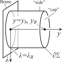
Figure 3: Integration surface.

Firstly, the integration on the “side” of $\partial\Sigma$, that is the cylindrical surface $\lambda=\lambda_{B}$, is given as

$$~{}2\times\frac{1}{8\pi G_{5}}\oint_{\text{side}}\!\!\!\!\!\!dyd\theta d\phi\sqrt{-\bar{g}}\left[K^{\tau\lambda\nu\beta}{}_{;\beta}\bar{\xi}_{\nu}-K^{\tau\beta\nu\lambda}\bar{\xi}_{\nu;\beta}\right]$$

$$=\frac{\tilde{k}^{4}\lambda_{B}^{2}}{k^{4}G_{5}}\int^{y_{B}}_{y_{b}}\!\!\!dy\cosh^{4}\left(ky\right)\left[K^{\tau\lambda\nu\beta}{}_{;\beta}\xi_{\nu}-K^{\tau\beta\nu\lambda}\xi_{\nu;\beta}\right]\bigg{|}_{\lambda=\lambda_{B}}\;.$$ (21)

The factor two in the left-hand side is multiplied since the same contribution comes from the both sides of the brane. For the perturbation due to the black hole $h^{\text{BH}}_{\mu\nu}$, the integrand of Eq. (21) becomes $\mathcal{O}\left(\lambda_{B}^{-1}\right)$ and thus the integral vanishes in the limit $\lambda_{B}\to\infty$. On the other hand, the contribution from the gauge perturbation $h^{\zeta}_{\mu\nu}$ becomes

$$\lim_{\lambda_{B},y_{B}\to\infty}\frac{\tilde{k}^{4}\lambda_{B}^{2}}{k^{4}G_{5}}\int^{y_{B}}_{y_{b}}\!\!\!dy\cosh^{4}\left(ky\right)\left[K^{\tau\lambda\nu\beta}{}_{;\beta}\xi_{\nu}-K^{\tau\beta\nu\lambda}\xi_{\nu;\beta}\right]$$

$$~{}~{}~{}~{}=-\frac{\tilde{k}^{3}}{2k^{4}G_{5}}\left[\cosh^{2}(ky)\left(\frac{G^{\prime}\cosh^{2}(ky)}{\tilde{k}}-\frac{5k^{2}\delta y_{3}F}{\tilde{k}^{2}}\right)\right]^{y=\infty}_{y=y_{b}}=-\frac{4\delta y_{3}}{\tilde{k}G_{5}}=\frac{4\tilde{k}^{3}\sin^{3}\chi_{0}}{k^{5}G_{5}}\delta\chi_{4}~{},$$ (22)

where we used the boundary conditions for $F$ and $G^{\prime}$ as well as $(\tilde{k}/k)\cosh\left(ky_{b}\right)=1$.

Next, the integration on the “caps” of the cylinder, that is the surfaces $y=\pm y_{B}$, is given as

$$~{}2\times\frac{1}{8\pi G_{5}}\oint_{\text{cap}}\!\!\!\!\!d\lambda d\theta d\phi\sqrt{-\bar{g}}\left[K^{\tau y\nu\beta}{}_{;\beta}\bar{\xi}_{\nu}-K^{\tau\beta\nu y}\bar{\xi}_{\nu;\beta}\right]$$

$$=\frac{\tilde{k}^{4}\cosh^{4}\left(ky_{B}\right)}{k^{4}G_{5}}\int_{0}^{\lambda_{B}}\!\!\!d\lambda\,\lambda^{2}\left[K^{\tau y\nu\beta}{}_{;\beta}\bar{\xi}_{\nu}-K^{\tau\beta\nu y}\bar{\xi}_{\nu;\beta}\right]\bigg{|}_{y=y_{B}}\;.$$ (23)

$h^{\text{BH}}_{\mu\nu}$ gives a nonzero contribution to this integral as

$$\lim_{\lambda_{B},y_{B}\to\infty}\frac{\tilde{k}^{4}\cosh^{4}\left(ky_{B}\right)}{k^{4}G_{5}}\int_{0}^{\lambda_{B}}\!\!\!d\lambda\,\lambda^{2}\left[K^{\tau y\nu\beta}{}_{;\beta}\xi_{\nu}-K^{\tau\beta\nu y}\xi_{\nu;\beta}\right]$$

$$~{}~{}~{}=\int_{0}^{\infty}\!\!\!d\lambda\,\frac{3\mu\tilde{k}^{4}\left(1-v^{2}\right)^{2}\lambda^{2}}{2kG_{5}\big{(}\tilde{U}^{1/2}+v\big{)}^{4}}=\frac{\mu\tilde{k}}{4kG_{5}\sin\chi_{0}}\left\{3\chi_{0}+\sin\chi_{0}\cos\chi_{0}\left(2\cos^{2}\chi_{0}-5\right)\right\}\;,$$ (24)

while $h^{\zeta}_{\mu\nu}$ gives no contribution since $\zeta^{\mu}$ vanishes for $y\to\infty$.

After all, we obtain an expression of the Abbott-Deser mass as

$$M=\frac{1}{k^{2}G_{5}}\left[\frac{4\tilde{k}^{3}\sin^{3}\chi_{0}}{k^{3}}\,\delta\chi_{4}+\frac{\mu k\tilde{k}}{4\sin\chi_{0}}\left\{3\chi_{0}+\sin\chi_{0}\cos\chi_{0}\left(2\cos^{2}\chi_{0}-5\right)\right\}\right]~{}~{},$$ (25)

which is totally expressed in terms of the quantities in the global coordinates. Once we construct an initial data numerically, its mass can be calculated by reading out $\chi_{0}$ and $\delta\chi_{4}$ from the brane trajectory and plugging those into the above formula.

Let us comment on the tensionless limit of the mass formula, that is the limit to make $\chi_{0}\to\pi/2$ and $k\to\tilde{k}$ simultaneously. In this limit, the five-dimensional system reduces to an AdS-Schwarzschild black hole with a tensionless brane on its equator plane, which do not contribute to the mass at all. This limit yields $M=3\pi\mu/8G_{5}$, which is an ordinary mass formula of a five-dimensional AdS-Schwarzschild black hole [17].

4 Analysis

In this and the next sections, we analyze our floating black hole initial data in the KR model using the Abbott-Deser mass we obtained in the previous section. We firstly summarize the properties of the initial data in this section. In Sec. 4.1, we calculate the mass of the initial data for fixed values of entropy to study thermodynamic stability of the system in a microcanonical ensemble. In Sec. 4.2, we estimate how an initial data is close to a static solution by observing additional matter that we have to put on the brane to make it static.

4.1 Local extrema of entropy

In this subsection, we calculate the Abbott-Deser mass of the initial data and try to find an initial data that is close to a static solution. To be more precise, we try to find an initial data that realizes maximum entropy keeping its mass fixed. The logic behind this search is as follows. If we have a set of all possible time-symmetric initial data, the all static solutions must be contained in this set since a static solution is also time-symmetric. Since we have the area increase law of the event horizon, a time-symmetric initial data that realizes the maximum entropy must be a static solution. Of course we can search only a finite region of the initial data phase space, and hence the initial data that realizes the maximum entropy in our initial data family is not necessarily static. Nevertheless, we can expect it to reflect some properties of a static solution since it satisfy some of the necessary conditions of a static solution. We later compare this initial data with maximum entropy to a four-dimensional static CFT star.

As we mentioned in Sec. 2 briefly, we focus on the regime that the five-dimensional model is only slightly detuned from the RS model, i.e. $\tilde{k}/k\ll 1$, in this paper. In the following numerical analysis, we set $\tilde{k}/k=1/100$. Every results are almost irrelevant to this ratio if it is smaller than this value. For technical convenience, we search initial data that minimize the mass keeping the entropy fixed instead of searching the one that maximize the entropy for fixed mass, since the former is much simpler to implement in our initial data construction method. This search is totally equivalent to the search for the entropy-maximum initial data keeping the mass fixed.

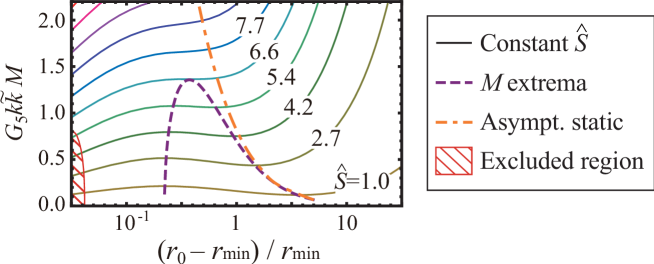
Figure 4: Plot of mass $M$ for initial data sequences for fixed values of entropy $\hat{S}\equiv G_{5}(k\tilde{k})^{3/2}S$ for $\tilde{k}/k=1/100$. The horizontal axis shows the distance between the brane position on the rotational axis $r_{0}$ and the lower bound for $r_{0}$, $r_{\text{min}}$, where $r_{\text{min}}$ takes different values on different $\hat{S}$ constant sequences. A sequence for $\hat{S}$ smaller than $6.6$ possesses a local maximum and a minimum of mass. By connecting the local extrema of various sequences, we obtain the dashed line in the plot, which have a peek at $G_{5}k\tilde{k}M=1.4$ . The dash-dotted line represents initial data that becomes static in the asymptotic region. When the entropy is small, we see that the initial data that realizes the mass local minimum is almost asymptotically static. In any initial data sequence, the mass local maximum is always further than the local minimum from the point of the asymptotically-static initial data. The initial data in the shaded region possesses an outer apparent horizon, and this region is excluded from the analysis in this paper.

Figure 4 shows variance of the mass $M$ for sequences of fixed values of the entropy $S=A_{\text{BHs}}/4G_{5}$. We can see that a mass minimum and a maximum appear in each sequence for small entropy, while no extrema appears in a sequence for large entropy. At $G_{5}(k\tilde{k})^{3/2}S=6.6$, sequences of mass maximum and of mass minimum annihilate in pair. The disappearance of mass local minimum suggests that the thermodynamical stability in a microcanonical ensemble changes from stable to unstable there, and that a transition from bulk floating black hole to the brane-localized black holes occurs near this point.

Figure 5: Schematic picture of the effective potential for a small particle in the bulk of the KR model.

Let us further investigate the sequence of mass extrema. The line of mass local minima is smoothly connected with the line of mass local maxima, as is shown in Fig. 4. We can interpret it in the Newtonian sense as follows. When the floating black hole is sufficiently small, it will be approximated by a small particle of mass $M_{sp}$. Then, there are two positions in the bulk where this small particle can stay in a static manner: the potential minimum, that is the throat of the AdS₅ at which the warp factor is minimized, and the near brane point at which the brane’s repulsion force $a=k$ is cancelled by the gravitational attraction due to its mirror image behind the brane $a\sim-G_{5}M_{sp}/(2d)^{3}$, where $d$ is proper distance between the small particle and the brane. We show a schematic picture of the effective gravitational potential for a small particle in Fig. 5. See also [23, 24] for detail about this effective potential. When the small particle sits at the latter point near the brane, the system is in unstable equilibrium and the energy will be maximized. For example, mass-maximum initial data in the sequence of $G_{5}(k\tilde{k})^{3/2}S=2.0\times 10^{-3}$ has black holes with $G_{5}k\tilde{k}M_{sp}\sim G_{5}k\tilde{k}M/2=1.3\times 10^{-2}$, and then the position of the unstable equilibrium is estimated as $\tilde{k}d=\tilde{k}(G_{5}M_{sp}/8k)^{1/3}=5.4\times 10^{-3}$. This value is roughly equal to the actual proper distance between the brane and the black hole in our initial data, which is $4.4\times 10^{-3}$. As the floating black hole becomes large, those two points of equilibrium get closer to each other and finally annihilate. This annihilation corresponds to the turn over of the mass-extrema sequence in Fig. 4.

We find some initial data, especially those with small floating black hole located very near the brane, have an outer apparent horizon. We exclude such initial data in this paper to focus only on the bulk floating black hole solutions. We also mention that any initial data with maximum or minimum mass seems not to have an outer apparent horizon, at least for $G_{5}(k\tilde{k})^{3/2}S\gtrsim 1$.

4.2 Difference of initial data from static solutions

In our initial data construction, the brane does not become static in the GN coordinates by itself in general. Since we would like to compare the initial data with static CFT stars, we have to know how “far” an initial data is from a static state. For this purpose, we try to find asymptotically-static initial data, in which the brane becomes static in the asymptotic region.

Since the transformation (14) maps a static brane in the GN coordinates to a brane with $\chi_{0}=\pi/2$ in the AdS global coordinates and it does not mix the temporal coordinate with the spatial coordinates, a brane with $\chi_{0}=\pi/2$ becomes static at $\lambda\to\infty$. We denote an initial data with such a brane as an asymptotically-static initial data. We can find such an initial data uniquely in an initial data sequence for a fixed $S$. The dash-dotted line in Fig. 4 is of the sequence of such asymptotically-static initial data. In the figure, we find that the mass-minimum initial data are approximately asymptotically static when the entropy is small. We can also see that the mass-maximum initial data is always more distant from the asymptotically static one than the mass-minimum one with the same entropy.

The result that a mass-minimum initial data becomes closer to an asymptotically-static initial data for small bulk black holes is a natural one in the following sense; When the bulk black hole is small, it will be approximated by a small particle. If we place it at the potential minimum of the bulk gravitational field, it will stay there in a static manner without disturbing the background geometry. Then, the whole system including the small particle will be almost static, and it approximates the asymptotically-static initial data well.

We can assess the staticity of an initial data in a more quantitative way as follows. When a brane in an initial data is dynamical, we can make it static by putting some additional matter on it. The amount of this additional matter will be a good indicator of staticity. By comparing it with the effective energy-momentum tensor or the cosmological constant on the brane, we can see to what extent the initial data is close to a static solution.

The additional matter to make the brane static is estimated as follows. The four-dimensional Einstein equations on the brane are given by

$$G^{\text{4D}}_{ab}+\Lambda_{4}g^{\text{4D}}_{ab}=-\mathcal{E}_{ab}~{}~{},$$ (26)

where $\mathcal{E}_{ab}\equiv C_{\mu\lambda\nu\rho}\gamma^{\mu}_{~{}a}s^{\lambda}\gamma^{\nu}_{~{}b}s^{\rho}$ is the bulk Weyl tensor projected onto the brane and $G^{\text{4D}}_{ab}$ is the Einstein tensor for four-dimensional metric induced on the brane [29]. Effective energy density and pressure on the brane are defined using four-dimensional Newton constant $G_{4}=kG_{5}$ as $\rho\equiv\mathcal{E}^{\tau}_{~{}\tau}/8\pi G_{4}$ and $P_{i}\equiv-\mathcal{E}^{i}_{~{}i}/8\pi G_{4}$ for $i=\lambda$ and $\theta$, respectively. To keep the brane static, we have to add an additional energy-momentum tensor $\delta T_{ab}$, which replaces Eq. (26) with

$$G^{\text{4D}}_{ab}+\Lambda_{4}g^{\text{4D}}_{ab}=-\mathcal{E}_{ab}+8\pi G_{4}\delta T_{ab}~{}~{}.$$ (27)

Now that the brane is static, the induced metric on the brane is given by

$$ds^{2}=g^{\text{4D}}_{ab}dx^{a}dx^{b} =-Udt^{2}+\left(\frac{1}{U}+r^{2}\sin^{2}\chi\right)dr^{2}+r^{2}\sin^{2}\chi\left(d\theta^{2}+\sin^{2}\theta d\phi^{2}\right)$$

$$=-\biggl{(}\frac{\tilde{k}}{k}\biggr{)}^{2}Ud\tau^{2}+\frac{1}{\tilde{U}^{\prime}}d\lambda^{2}+\lambda^{2}\left(d\theta^{2}+\sin^{2}\theta d\phi^{2}\right)~{}~{},$$ (28)

where $\tilde{U}^{\prime}$ is defined by the last equality of this equation. Using this metric, $\delta T_{ab}$ is obtained via Eq. (27). By comparing $\delta T_{\mu\nu}$ with $-\mathcal{E}_{ab}/8\pi G_{4}$ or $\Lambda_{\text{4}}$, we can estimate how the brane is close to a static state. We note here that $\delta\rho\equiv-\delta T^{\tau}_{~{}\tau}$ automatically vanishes since the Hamiltonian constraint is satisfied. Below, we investigate properties of the nontrivial components $\delta P_{i}\equiv\delta T^{i}_{~{}i}$.

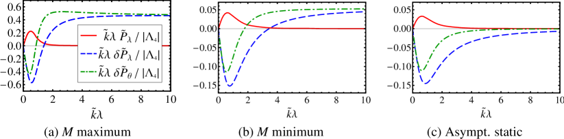
Figure 6: Distributions of effective pressure $\tilde{P}_{\lambda}\equiv 8\pi G_{4}P_{\lambda}$ and additional pressure $\delta\tilde{P}_{i}\equiv 8\pi G_{4}P_{i}$ for $i=\lambda$ and $\theta$. The panels (a) and (b) show the distributions for initial data with maximum and minimum $M$ of an initial data sequence for $G_{5}(k\tilde{k})^{3/2}S=4.3$ , and the panel (c) shows that for the asymptotically-static initial data in the same sequence. The all quantities are normalized by $\Lambda_{4}$. $\delta P_{i}$ decays as $\lambda^{-1}$ and is much smaller for the asymptotically-static initial data than the others. Note that scale of the vertical axis in the panel (a) is much larger than those of the other panels.

In Fig. 6, we plot distributions of effective matter and additional matter for mass-maximum, mass-minimum and asymptotically-static initial data in the initial data sequence for $G_{5}(k\tilde{k})^{3/2}S=4.3$ . These plots shows that additional matter of much larger amount is necessary to make the mass-maximum initial data static compared to the mass-minimum and asymptotically-static ones. Note that scale of the vertical axis of Fig. 6(a) is much larger than those of Figs. 6(b) and 6(c). This confirms that the mass-minimum initial data is closer to a static solution compared to the mass-maximum one.

This fact about mass-maximum initial data indicates that the genuine static solution of the floating black hole in unstable equilibrium, even if existed, is far from the initial data we constructed. The reason for it may be as follows: the floating black hole in the unstable equilibrium is highly deformed by the self-gravity due to its mirror image behind the brane and the repulsion force due to the brane, and then it cannot be well approximated by an AdS-Schwarzschild black hole we used in the initial data construction.

5 Comparison with Four-dimensional CFT stars

Using the tools prepared in the previous sections, we conduct a comparison between the five-dimensional floating black hole initial data and the four-dimensional CFT stars.

We firstly illustrate the numerical construction method of the CFT star configuration and summarize basic properties of the CFT stars in Sec. 5.1, though the construction method is originally given by [30] and a detailed analysis is done by [24]. In Secs. 5.2 and 5.3, we compare the sequence of the CFT stars with the sequence of initial data at mass extrema, which is expected to mimic a sequence of five-dimensional static solutions. We compare the structure of the whole sequences in Sec. 5.2, and after that we focus on some specific solutions in the sequences in Sec. 5.3.

5.1 Construction method

When the temperature is sufficiently high compared to the characteristic energy scale on the brane, $T\gg\tilde{k}$, we can approximate the CFT with radiation fluid, whose energy density is given by $\rho=aT_{\text{loc}}^{~{}~{}4}$ where $T_{\text{loc}}$ is the local temperature determined from the global temperature $T$ as $T_{\text{loc}}=(-g_{\tau\tau})^{-1/2}T$. In our setting, two sets of the CFT reside on the brane since we have two bulk regions on each side of the brane. Then, the radiation density constant is given by $a=(\pi^{2}/30)\times 15N^{2}\times 2=\pi^{3}/2k^{3}G_{5}$, where the factor $15=6+2+(7/8)\times 8$ is the effective spin state number of the CFT multiplets: six real scalars, one vector and four Weyl fermions.

Assuming spherical symmetry and staticity, general four-dimensional metric can be parametrized as

$$ds^{2}=-e^{2\psi}V(\lambda)dt^{2}+V(\lambda)^{-1}d\lambda^{2}+\lambda^{2}\left(d\theta^{2}+\sin^{2}\theta d\phi^{2}\right)$$ (29)

and $V=1+\tilde{k}^{2}\lambda^{2}-2m(\lambda)/\lambda$. We require that $\lim_{\lambda\to\infty}\psi=0$ to realize asymptotically AdS₄ spacetime and $m(\lambda=0)=0$ to maintain the regularity at the center. Then, the four-dimensional Einstein equations for energy-momentum tensor of the radiation fluid $T^{\mu}_{~{}\nu}=\text{Diag}[-\rho,p,p,p]$ with $\rho=3p=aT^{4}e^{-4\psi}V^{-2}$ are given by

$$\frac{dm}{d\lambda}=4\pi\lambda^{2}\rho~{},\qquad\frac{d\rho}{d\lambda}=\frac{-4\rho\left(G_{4}m+4\pi G_{4}\lambda^{3}\rho/3+\tilde{k}^{2}\lambda^{3}\right)}{\lambda^{2}+\tilde{k}^{2}\lambda^{4}-2G_{4}\lambda m}~{}.$$ (30)

Assuming regularity at $\lambda=0$ and giving central density $\rho(\lambda=0)\equiv\rho_{c}$, we can solve these equations to obtain one-parameter family of solutions $m(\rho_{c};\lambda)$ and $\rho(\rho_{c};\lambda)$. Four-dimensional mass is given by $M=\lim_{\lambda\to\infty}m(\lambda)$. Using the solutions $m$ and $\rho$, the global temperature and the metric function $\psi$ can be obtained from the expression of the energy density as $T=\lim_{\lambda\to\infty}(\rho V^{2}/a)^{1/4}$ and $\psi=(1/4)\log(aT^{4}/\rho V^{2})$. The total entropy of the system $S$ can be obtained by integrating proper entropy density $s=(4/3)aT_{\text{loc}}^{~{}~{}3}$. We note this $S$ satisfies the thermodynamic first law $dM=TdS$.

Since the CFT resides not only on the brane but also on the AdS boundaries, we have to add their contributions to $M$ and $S$. For convenience of the derivation, let us consider from the five-dimensional point of view. We introduce a second AdS brane of curvature $\tilde{k}_{b}$ in the bulk near the AdS boundary, and consider the CFT on it. Let us refer to this CFT on the second brane as CFT2. In the GN coordinates (13), such a brane is at $y=y_{b}$ such that $(\tilde{k}/k)\cosh(ky_{b})=\tilde{k}/\tilde{k}_{b}$. The induced geometry on that second brane is given by

$$ds^{2}=\biggl{(}\frac{\tilde{k}}{\tilde{k}_{b}}\biggr{)}^{2}\left(-\tilde{U}d\tau^{2}+\frac{d\lambda^{2}}{\tilde{U}}+\lambda^{2}d\Omega_{\text{II}}\right)=-\tilde{U}_{b}d\tau_{b}^{2}+\frac{d\lambda_{b}^{2}}{\tilde{U}_{b}}+\lambda_{b}^{2}d\Omega_{\text{II}}~{}~{},$$ (31)

where $\tilde{U}=1+\tilde{k}^{2}\lambda^{2}$ and $\tilde{U}_{b}=1+\tilde{k}_{b}^{2}\lambda_{b}^{2}$. From this equation, we find that the coordinates on the brane $\tau_{b}$ and $r_{b}$ are related to those in the GN coordinates as

$$\tau_{b}/\tau=\lambda_{b}/\lambda=\tilde{k}/\tilde{k}_{b}~{}~{}.$$ (32)

The CFT on the second brane have to be in thermal equilibrium with that on the first brane. Hence, the global temperature on the second brane, which is the equilibrium temperature measured by $\tau_{b}$, is given by $T_{b}=(\tau/\tau_{b})T=(\tilde{k}_{b}/\tilde{k})T$. We note here that the radiation fluid approximation is valid also on the second brane since this relation and the condition $T\gg\tilde{k}$ implies $T_{b}\gg\tilde{k}_{b}$. Since the CFT decouples from gravity in the limit to take the second brane to the AdS boundary, we can neglect the back reaction of the radiation to the background geometry. Then, energy density and entropy density are given by $\rho=aT^{~{}~{}4}_{\text{loc}}$ and $s=(4/3)aT_{\text{loc}}^{~{}~{}3}$ with $T_{\text{loc}}=\tilde{U}_{b}^{-1/2}T_{b}$, and total mass and entropy are given by

$$M_{b}=\int_{0}^{\infty}4\pi\lambda_{b}^{2}\rho\,d\lambda_{b}=\frac{\pi^{2}a}{\tilde{k}^{4}}\tilde{k}_{b}T^{4}~{}~{},\qquad S_{b}=\int_{0}^{\infty}4\pi\lambda_{b}^{2}s\;\sqrt{g_{\lambda_{b}\lambda_{b}}}d\lambda_{b}=\frac{4\pi^{2}a}{3\tilde{k}^{3}}T^{3}~{}~{}.$$ (33)

Due to the rescaling of the time coordinate (32), an observer on the first brane measures the mass and entropy on the second brane as $M_{\text{CFT2}}=(\tilde{k}/\tilde{k}_{b})M_{b}$ and $S_{\text{CFT2}}=S_{b}$. These $M_{\text{CFT2}}$ and $S_{\text{CFT2}}$ are independent of $\tilde{k}_{b}$ and of the brane position, we can safely take the limit to send the second brane to the AdS boundary making $\tilde{k}_{b}\to 0$. Note that there are two AdS boundaries in our setting, and their contributions can be taken into account simply by setting the radiation density constant $a$ to $\pi^{3}/2k^{3}G_{5}$ in the above calculation. Below in this paper, we always include these $M_{\text{CFT2}}$ and $S_{\text{CFT2}}$ to the total mass $M$ and entropy $S$.

By the way, the radiation fluid approximates a weak-coupling CFT, though the five-dimensional gravity is expected to be dual to a strongly-coupled CFT. It is known that this gap can be filled by reducing the CFT’s degrees of freedom $N^{2}=\pi/2k^{2}G_{4}$ to $(3/4)\times N^{2}$. Inclusion of this factor can be easily performed as follows. When we change $G_{4}$ and $k$, $M$, $S$, $T$, $\rho$, and $G_{5}$ are rescaled as $M\propto G_{4}^{-1}$, $\rho\propto G_{4}^{-1}$, $T\propto k^{1/2}$, and $S\propto G_{4}^{-1}k^{-1/2}$, respectively. Using this scaling, we find that, for example, each quantity is rescaled as $M\to M$, $\rho\to\rho$, $T\to(3/4)^{-1/4}T$, and $S\to(3/4)^{1/4}S$ if we fix $G_{4}$ to be constant and introduce the factor $3/4$ by changing $k$. We always take this factor into account in the analysis of CFT stars hereafter in this paper.

Let us summarize features of the CFT star solution sequence. When $\rho_{c}$ is lower than the four-dimensional cosmological constant $\Lambda_{\text{4}}=-3\tilde{k}^{2}$, the background geometry does not change much from the pure AdS₄, and the total mass and entropy are proportional to $\rho_{c}$ and $\rho_{c}^{3/4}$, respectively. In this regime, the CFT stars have positive specific heat and thus they are thermodynamically stable. Increasing $\rho_{c}$, the total mass and the entropy is maximized for the same critical $\rho_{c}$. The system becomes thermodynamically unstable for $\rho_{c}$ larger than this critical value if the system is in a microcanonical ensemble.

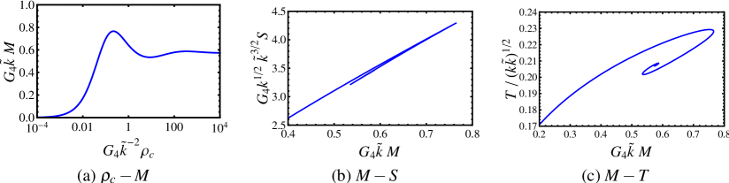
Figure 7: Plots of characteristic quantities of the CFT star sequence. The panel (a) shows the behavior of $M$ against $\rho_{c}$. $M$ is maximized at $G_{4}\rho_{c}/\tilde{k}^{2}=0.22$, and it shows oscillatory behavior for larger $\rho_{c}$. The system becomes thermodynamically unstable for $\rho_{c}$ larger than this critical value if the system is in a microcanonical ensemble. The panels (b) and (c) show variance of $S$ and $T$ against $M$, respectively. In the both panels, the curves turn around at the critical $\rho_{c}$ and converges to a point in the limit of infinite $\rho_{c}$.

In the limit of infinite central density, the radiation fluid may gravitationally collapse and form a small black hole. In the AdS spacetime, this black hole can settle into thermodynamical equilibrium with its own Hawking radiation, since the gravitational potential due to the negative cosmological constant works as an effective cavity. We call this system in thermal equilibrium as a quantum-corrected black hole. It is shown that the CFT star sequence is smoothly connected to the quantum-corrected black hole sequence in the limit of infinite central density [24]. This quantum-corrected black holes are conjectured to be dual to five-dimensional brane-localized black holes, though we do not pursue this duality between them in this paper.

5.2 Comparison of the solution sequences

In this and the next sections, we juxtapose the CFT star sequence with the sequence of the five-dimensional floating black hole initial data at local extrema of mass. Firstly, we compare the whole solution sequences of the four-dimensional CFT picture and the five-dimensional KR picture. In Fig. 8, we show the relation of $M$, $S$ and $T$ along the solution sequences. The curves for the CFT star sequence are the same as those in Figs. 7(b) and 7(c). For initial data, the temperature $T$ is not well-defined since the information of the lapse function, which is crucial for the temperature determination, is missing. We thus define $T$ of initial data using the thermodynamic first law $T\equiv dM/dS$. This $T$ will approximate the physical temperature of the system if the initial data is close to a static solution.

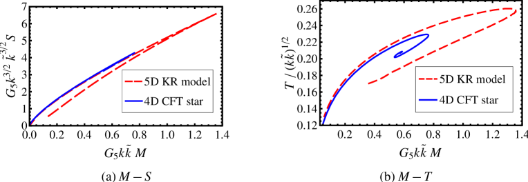
Figure 8: $M-S$ and $M-T$ diagram for solution sequences. The dashed line is of the five-dimensional initial data at the mass extrema, and the solid line is of the four-dimensional CFT stars. In the left panel for $M-S$ relation, the curves of the two pictures have sharp edges at certain critical values of mass, which are $G_{5}k\tilde{k}M=0.77$ for the four-dimensional CFT star sequence and $1.4$ for the five-dimensional initial data sequence. We can see qualitative similarities between the curves of the two pictures in each panel, while there are quantitative differences. The curves of the two pictures match each other well in the range from the origin to the critical $M$ of the CFT star sequence. The deviation of the two curves becomes significant in the parameter region where the initial data become far from static solutions (see Fig. 4).

In the plot, we can see some common features between the curves of the initial data and of the CFT stars. The curves near the origin of the graph correspond to the sequences of small floating black holes or low central density CFT stars. As we increase the black hole size or the central density, they approach the critical points at which $M$ is maximized, and then they turn around. In this sense, thermodynamic phase structures are qualitatively the same between the two pictures. Since the Hawking-Page transition occurs in the four-dimensional picture and a transition of the bulk black hole configuration is suggested to occur (see Sec. 4.1) at the critical points, this result suggests that these transitions in the two pictures are holographic dual of each other.

A quantitative difference appears in the part of the sequences after the critical point of the CFT star sequence, which is at $(G_{5}k\tilde{k}M,G_{5}(k\tilde{k})^{3/2}S,T/(k\tilde{k})^{1/2})=(0.77,4.3,0.23)$ . No feature appears in the initial data sequence at the critical point of the CFT star sequence, and the critical point in the five-dimensional initial data sequence appears at $(G_{5}k\tilde{k}M,G_{5}(k\tilde{k})^{3/2}S,T/(k\tilde{k})^{1/2})=(1.4,6.6,0.26)$ . A conceivable reason for this mismatch is that the initial data in that parameter region is far from a static state. Figures 4 and 6 show that mass-maximum initial data are very different from static solutions, and deviation of an initial data from a static solution becomes larger as we move along the sequence toward the mass-maximum initial data. When the staticity is largely violated, the duality between the mass-extremum initial data and the static CFT stars will break down. In fact, the deviation of the initial data from asymptotically-static solutions becomes manifest for $G_{5}(k\tilde{k})^{3/2}S\gtrsim 4$ as is shown in Fig. 4. This naive expectation will be confirmed using five-dimensional static solutions, which are yet to be constructed.

5.3 Comparison of solutions

Next, we compare some specific solutions in the both pictures to investigate to what extent the duality holds. In the CFT picture, we take a CFT star solution at the critical point, at which $M$ is maximized, as a representative. In the KR picture, we choose a mass-minimum initial data which share the same $M$ with that CFT star solution. In other words, we pick up solutions near the point $(G_{5}k\tilde{k}M,G_{5}(k\tilde{k})^{3/2}S)=(0.77,4.3)$ in Fig. 8(a) from both sequences, and compare those solutions to each other. We compare the energy-momentum tensor of the four-dimensional CFT star $T_{ab}$ with the effective energy-momentum tensor $-\mathcal{E}_{ab}/8\pi G_{5}$ between such solutions. This effective energy-momentum tensor is traceless by definition, which is a common property with $T_{ab}$ of the radiation fluid. We would like to clarify other similarities between them in this subsection. Adding to the energy-momentum, we also compare the four-dimensional geometries between the two pictures.

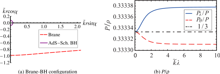
Figure 9: Initial data at the data point $(G_{5}k\tilde{k}M,G_{5}(k\tilde{k})^{3/2}S)=(0.77,4.3)$ and the effective pressure on its brane. The left panel shows the configurations of the brane and the bulk floating black hole. The bulk region is the upper side of the brane, and the lower side of the brane is to be cut away. The right panel shows the ratios of the effective pressure components $P_{i}$ in radial and angular directions to the effective energy density $\rho$ on the brane. Relative difference of those ratios from $1/3$ is smaller than a percent. It shows that the effective pressure on the brane is almost isotropic.

In Fig. 9(a), we show the configuration of the brane and the floating black hole for the data point mentioned above. As a first check, we study properties of the effective pressure distribution in Fig. 9(b). We find that the pressure is approximately isotropic, i.e. $P_{\lambda}\simeq P_{\theta}$, similarly to the radiation fluid. Since the brane’s effective energy-momentum tensor is traceless, i.e. $\rho=P_{\lambda}+2P_{\theta}$, this result means that the equation of state of the effective matter is quite similar to the radiation fluid.

Figure 10: Comparison of characteristic quantities at the data point $(G_{5}k\tilde{k}M,G_{5}(k\tilde{k})^{3/2}S)=(0.77,4.3)$ . The left panel shows distributions of effective energy density on the brane and of the CFT star. The right panel shows the metric function $m(\lambda)$ in $\tilde{U}=1+\tilde{k}^{2}\lambda^{2}-2G_{4}m(\lambda)/\lambda$. In both figures, we can see that the curves of the two pictures are close for a large $\lambda$, while they deviate near the center $\lambda=0$.

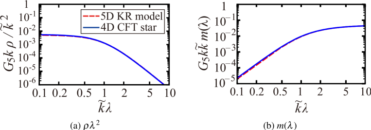
Figure 11: Comparison of characteristic quantities at the data point $(G_{5}k\tilde{k}M,G_{5}(k\tilde{k})^{3/2}S)=(0.10,0.89)$ , at which the initial data is almost asymptotically static as we can see in Fig. 4. In this case, almost exact match is realized between $\rho$ or $m(\lambda)$ of the two pictures.

In Fig. 10, we compare radial profiles of energy density $\rho$ and the metric function $m(\lambda)$. Firstly, we compare $\rho$ of the two pictures in Fig. 10(a). We can see that the curves of the two pictures share common qualitative behaviors, such as power-law fall-off in the asymptotic region $\lambda\to\infty$. Secondary, Fig. 10(b) shows that the intrinsic geometry of the four-dimensional spacetime in the CFT picture is quite similar to that induced on the brane in the five-dimensional KR picture. Asymptotic values of $m(\lambda)$ in the two pictures are almost same, which is a non-trivial result since we tuned the total mass $M$ of the solutions to be common but did not tuned the value of $\lim_{\lambda\to\infty}m(\lambda)$ directly. Recall that $M$ of a CFT star is given by a sum of the asymptotic value of $m(\lambda)$ and the mass of the CFT2 as we explained in Sec. 5.1, and that $M$ of an initial data is not related directly to $m(\lambda)$ determined from the induced geometry on the first brane. These similarities between the two pictures supports the conjectured correspondence in the KR model. However, quantitative difference between the curves becomes big in the central region $\lambda\simeq 0$ as we can see in the both plots. We expect this discrepancy to be reduced if we use static solutions instead of initial data for comparison.

In Fig. 11, we show $\rho$ and $m(\lambda)$ for the data point $(G_{5}k\tilde{k}M,G_{5}(k\tilde{k})^{3/2}S)=(0.10,0.89)$, for which the mass-minimum initial data is almost equivalent to an asymptotically-static initial data (see Fig. 4). In this case, two pictures give almost exactly the same $\rho(\lambda)$ and $m(\lambda)$. This fact supports the above naive expectation that the coincidence will improve for five-dimensional static solutions.

6 Summary

Using the time-symmetric initial data, we showed that the Hawking-Page transition in a microcanonical ensemble on four-dimensional spacetime is well reproduced in the five-dimensional KR model as a transition of bulk black hole configuration. We found good agreements between those two pictures in thermodynamical phase structures and in some characteristic values such as energy density distributions or the intrinsic geometries. These results strongly suggest that the holographic description initially claimed in the RS model also holds in the KR model.

As a byproduct, we obtained a definition of conserved mass in the KR model by extending the definition of mass for asymptotically AdS spacetime by Abbott and Deser. We also gave an explicit mass formula for the initial data we constructed. This definition reproduces an ordinary mass formula for an AdS-Schwarzshilcd black hole. Since this definition of mass is valid even for dynamical spacetime, it will have a wide application to the analysis of gravitational phenomena in the KR model.

Although we used time-symmetric initial data in this study, it is definitely preferred to use static solutions to compare with static CFT stars, which will improve the agreement between the two pictures significantly. Such five-dimensional static solutions may be constructed only numerically. We will study this issue in our future work. In addition to that, it was conjectured in Ref. [8] that brane-localized black holes in the KR model are dual to four-dimensional quantum-corrected black holes, whose properties are intensively studied in Ref. [24]. Investigation of this duality using five-dimensional initial data or static solutions will clarify further the properties of the holography in the KR model.

Another ambitious future work is to test the holography of this type in dynamical set-up using the technique of numerical relativity in higher-dimensional spacetime, which is now available in asymptotically flat spacetime [31, 32]. The initial data studied in this paper also provide a steady step toward this project. We would like to pursue it in the future.

- [1] J. M. Maldacena, Adv. Theor. Math. Phys. 2 (1998) 231 [Int. J. Theor. Phys. 38 (1999) 1113] [arXiv:hep-th/9711200].
- [2] L. Randall and R. Sundrum, Phys. Rev. Lett. 83, 4690 (1999) [arXiv:hep-th/9906064].
- [3] E. Witten, remarks at ITP Santa Barbara conference, “New Dimensions in Field Theory and String Theory,” http://www.itp.ucsb.edu/online/susy_c99/discussion/.
- [4] H. L. Verlinde, Nucl. Phys. B 580 (2000) 264 [arXiv:hep-th/9906182].
- [5] S. S. Gubser, Phys. Rev. D 63 (2001) 084017 [arXiv:hep-th/9912001].
- [6] S. W. Hawking, T. Hertog and H. S. Reall, Phys. Rev. D 62 (2000) 043501 [arXiv:hep-th/0003052].
- [7] T. Shiromizu and D. Ida, Phys. Rev. D 64 (2001) 044015 [arXiv:hep-th/0102035].
- [8] T. Tanaka, Prog. Theor. Phys. Suppl. 148 (2003) 307 [arXiv:gr-qc/0203082].
- [9] R. Emparan, A. Fabbri and N. Kaloper, JHEP 0208 (2002) 043 [arXiv:hep-th/0206155].
- [10] H. Kudoh, T. Tanaka and T. Nakamura, Phys. Rev. D 68 (2003) 024035 [arXiv:gr-qc/0301089].
- [11] T. Tanaka, arXiv:gr-qc/0402068.
- [12] A. L. Fitzpatrick, L. Randall and T. Wiseman, JHEP 0611 (2006) 033 [arXiv:hep-th/0608208].
- [13] L. Grisa and O. Pujolas, JHEP 0806 (2008) 059 [arXiv:0712.2786 [hep-th]].
- [14] N. Tanahashi and T. Tanaka, JHEP 0803 (2008) 041 [arXiv:0712.3799 [gr-qc]].
- [15] H. Yoshino, JHEP 0901 (2009) 068 [arXiv:0812.0465 [gr-qc]].
- [16] V. E. Hubeny, D. Marolf and M. Rangamani, arXiv:0908.2270 [hep-th].
- [17] R. Emparan and H. S. Reall, Living Rev. Rel. 11 (2008) 6 [arXiv:0801.3471 [hep-th]].
- [18] A. Karch and L. Randall, JHEP 0105 (2001) 008 [arXiv:hep-th/0011156].
- [19] A. Karch and L. Randall, JHEP 0106 (2001) 063 [arXiv:hep-th/0105132].
- [20] M. Porrati, JHEP 0204 (2002) 058 [arXiv:hep-th/0112166].
- [21] M. J. Duff, J. T. Liu and H. Sati, Phys. Rev. D 69 (2004) 085012 [arXiv:hep-th/0207003].
- [22] R. Bousso and L. Randall, JHEP 0204 (2002) 057 [arXiv:hep-th/0112080].
- [23] T. Tanaka, arXiv:0709.3674 [gr-qc].
- [24] K. Kashiyama, N. Tanahashi, A. Flachi and T. Tanaka, arXiv:0910.5376 [gr-qc].
- [25] A. Chamblin and A. Karch, Phys. Rev. D 72 (2005) 066011 [arXiv:hep-th/0412017].
- [26] S. Bhattacharyya, S. Lahiri, R. Loganayagam and S. Minwalla, JHEP 0809 (2008) 054 [arXiv:0708.1770 [hep-th]].
- [27] L. F. Abbott and S. Deser, Nucl. Phys. B 195 (1982) 76.
- [28] S. Creek, R. Gregory, P. Kanti and B. Mistry, Class. Quant. Grav. 23 (2006) 6633 [arXiv:hep-th/0606006].
- [29] T. Shiromizu, K. i. Maeda and M. Sasaki, Phys. Rev. D 62 (2000) 024012 [arXiv:gr-qc/9910076].
- [30] D. N. Page and K. C. Phillips, Gen. Rel. Grav. 17 (1985) 1029.
- [31] H. Yoshino and M. Shibata, arXiv:0907.2760 [gr-qc].
- [32] K. i. Nakao, H. Abe, H. Yoshino and M. Shibata, arXiv:0908.0799 [gr-qc].