Probing spectral properties of radio-quiet quasars searched for optical microvariability

Abstract

We obtained SDSS spectra for a set of 37 radio-quiet quasars (RQQSOs) that had been previously examined for rapid small scale optical variations, or microvariability. Their H$\beta$ and Mg ii emission lines were carefully fit to determine line widths (FWHM) as well as equivalent widths (EW) due to the broad emission line components. The line widths were used to estimate black hole masses and Eddington ratios, $\ell$. Both EW and FWHM are anticorrelated with $\ell$. The EW distributions provide no evidence for the hypothesis that a weak jet component in the RQQSOs is responsible for their microvariability.

1 Introduction

Over the past 15 years there have been rather extensive examinations of a significant sample of radio-quiet QSOs (RQQSOs) and Seyfert galaxies for small brightness changes (typically 0.02 mag) over short times (a few hours) (e.g., Stalin et al. 2004b; Carini et al. 2007; Ramírez et al. 2009). This phenomenon of microvariability, or intranight optical variability (INOV) was first confirmed for blazars (e.g., Miller, Carini & Goodrich 1989; Carini 1990) for which microvariability almost certainly arises from the relativistic jet (e.g., Marsher, Gear & Travis 1992), at least when the source is in an active state; however, in low states it is possible that rapid fluctuations are due to processes originating in or just above the accretion disc (for a review, see Wiita 2006). Since RQQSOs lack significant jets, the microvariability in radio-quiet objects may arise from processes on the accretion disc itself, and thus could possibly be used to probe the discs (e.g., Gopal-Krishna, Wiita & Altieri 1993; Stalin et al. 2004a; Kelly, Bechtold & Siemiginowska 2009).

Recently Carini et al. (2007) reported new observations for several sources and also compiled a sample of 117 objects from the literature which have been searched for microvariability (their Table 3). Of these, 47 are classified as Seyfert galaxies, 6 as broad absorption line (BAL) QSOs, and 64 as QSOs. In addition, in order to learn which classes might be the most fruitful for making further searchs for microvariability they also classified their sample in terms of following: redshift distribution; radio loudness, through $R$, the ratio of the radio [5 GHz] flux to the optical [4400Å] flux); optical magnitude, $m_{V}$; luminosity; and observing strategy. In their entire sample 21.4% of the objects were found to exhibit microvariability, but among objects classified as Seyfert galaxies, BAL QSOs and QSOs, microvariability was found in 17%, 50% and 23.2%, respectively (Carini et al. 2007). The observed high fraction of microvariations in BAL QSOs (although the sample is quite small) suggests that while planning microvariability studies to investigate the physical processes in or near the accretion disc, it might be worthwhile to invest more observing time on the BALQSO class.

With improvements in observation quality as well as in sample size, constraints on the models capable of producing the intranight variability have also improved over last decade. Recently, Czerny et al. (2008) have used non-simultaneous optical and X-ray data of 10 RQQSOs with confirmed INOV to compare observational constraints on the variability properties with the predictions of theoretical models such as: (i) irradiation of an accretion disc by a variable X-ray flux (e.g., Rokaki, Collin-Souffrin & Magnan 1993; Gaskell 2006); (ii) an accretion disc instability (e.g., Mangalam & Wiita 1993); (iii) the presence of a weak Doppler boosted jet, or “blazar component” (e.g., Gopal-Krishna et al. 2003). Their investigation suggests that a blazar component model yields the highest probability of detecting INOV.

In this blazar component scenario, spectral properties of the sources can play a crucial role in constraining the models further. For instance, if blazar components are dominating the variability of RQQSOs, then, due to the increase in the continuum level, one would expect emission lines to be diluted. Therefore smaller equivalent widths (EWs) of prominent emission lines such as H$\beta$ and Mg ii should be detected in sources that showed microvariability when compared to their average values in the whole sample. If we take the extreme case of BL Lacertae objects, which often lack observable emission lines and are usually defined as objects that have no emission line with an EW $\geq$5Å (e.g., Stickel et al. 1991; cf., Marchã et al. 1996), this dilution by the jet component is understood to be severe. So it becomes very important to test whether microvariability of RQQSOs has any correlation with spectral parameters such as EW and full width at half maximum (FWHM) of prominent emission lines. The H$\beta$ and Mg ii emission lines are very promising for such investigations, as these lines have also been found to be very useful in estimating other key parameters of AGN central engines such as black hole (BH) mass (e.g., McGill et al. 2008) and Eddington ratio (e.g., Dong et al. 2009a, 2009b). The average H$\beta$ EW of a large sample of quasars is found to be around 62.4Å (Foster et al. 2001), so any correlation of H$\beta$ EW or FWHM would not only give insight about the nature of variability, such as the presence or absence of blazar components, but also would be very useful for making a promising sample for future microvariability studies. Similarly the measurements of BH masses for RQQSOs that show microvariability may well be another important constraint on the models trying to understand the nature of their optical microvariability.

Here we have worked toward these goals by exploiting the optical spectra available from Sloan Digital Sky Survey (SDSS) Data Release 7 (DR7; Abazajian et al. 2009) with careful spectral modeling of the H$\beta$ and Mg ii emission line regions. First we aim to investigate any effect of these key spectral parameters (e.g., EW and FWHM) on microvariability of RQQSOs. Second we estimate other relevant AGN parameters such as the black hole mass, M_bh, and the Eddington ratio in the context of our RQQSOs sample, which has been extensively searched for microvariability.

The paper is organized as follows. Section 2 describes the data sample and selection criteria while Section 3 gives details of our spectral fitting procedure. In Section 4 we focus on BH mass measurements and in Section 5 we give estimates of Eddington ratios and of BH growth times. Section 6 gives a discussion and conclusions. Throughout, we have used a cosmology with $H_{\rm 0}$=70 km s^-1 Mpc^-1, $\Omega_{\rm M}$=0.3 and $\Omega_{\rm\Lambda}$=0.7.

Table 1: Our sample of radio-quiet QSOs and Seyfert galaxies from the compilation of Carini et al. (2007)

QSO Name	$z_{em}$	$\alpha_{2000}$			$\delta_{2000}$			mV	MV	Variable?	Class
Mrk 1014	0.163	01	59	50.2	$+$00	23	41	15.9	$-$23.8	Y	Sy 1
US 3150	0.467	02	46	51.9	$-$00	59	31	17.1	$-$25.0	N	NLS1
US 3472	0.532	02	59	37.5	$+$00	37	36	16.8	$-$25.7	N	QSO
Q J0751$+$2919	0.912	07	51	12.3	$+$29	19	38	16.2	$-$27.7	Y	QSO
PG 0832$+$251	0.331	08	35	35.9	$+$24	59	41	16.1	$-$25.5	Y	QSO
US 1420	1.473	08	39	35.1	$+$44	08	11	17.5	$-$27.3	N	QSO
US 1443	1.564	08	40	30.0	$+$46	51	13	17.2	$-$27.8	N	QSO
US 1498	1.406	08	42	15.2	$+$45	25	44	17.7	$-$26.7	N	QSO
US 1867	0.513	08	53	34.2	$+$43	49	01	16.9	$-$25.2	N	Sy 1
PG 0923$+$201	0.192	09	25	54.7	$+$19	54	04	15.5	$-$24.8	Y	Sy 1
PG 0931$+$437	0.456	09	35	02.6	$+$43	31	11	16.0	$-$26.4	N	QSO
PG 0935$+$416	1.966	09	38	57.0	$+$41	28	21	16.8	$-$28.8	N	QSO
CSO 233	2.030	09	39	35.1	$+$36	40	01	18.4	$-$27.3	N	QSO
CSO 18	1.300	09	46	36.9	$+$32	39	51	17.0	$-$27.9	N	QSO
US 995	0.226	09	48	59.4	$+$43	35	18	16.9	$-$23.4	Y	QSO
PG 0946$+$301	1.220	09	49	41.1	$+$29	55	19	16.2	$-$28.2	N	BAL QSO
CSO 21	1.190	09	50	45.7	$+$30	25	19	17.3	$-$27.3	N	QSO
TON 34	1.925	10	19	56.6	$+$27	44	02	15.7	$-$29.8	Y	QSO
PG 1049$-$005	0.357	10	51	51.5	$-$00	51	17	15.8	$-$25.7	N	Sy 1
TON 52	0.434	11	04	07.0	$+$31	41	11	17.3	$-$24.9	Y	QSO
PG 1206$+$459	1.155	12	08	58.0	$+$45	40	36	15.7	$-$28.4	N	QSO
UM 497	2.022	12	25	18.4	$+$02	06	57	17.7	$-$28.0	N	QSO
PG 1248$+$401	1.032	12	50	48.3	$+$39	51	40	16.3	$-$27.6	N	QSO
CSO 174	0.653	12	51	00.3	$+$30	25	42	17.0	$-$26.1	N	QSO
CSO 179	0.782	12	53	17.5	$+$31	05	50	17.0	$-$26.4	N	QSO
Q 1252$+$0200	0.345	12	55	19.7	$+$01	44	12	16.2	$-$25.3	Y	QSO
PG 1254$+$047	1.018	12	56	59.9	$+$04	27	34	16.3	$-$27.6	N	BAL QSO
PG 1259$+$593	0.472	13	01	12.9	$+$59	02	07	15.9	$-$26.2	N	QSO
PG 1307$+$085	0.154	13	09	47.0	$+$08	19	49	15.1	$-$24.6	N	Sy 1
PG 1309$+$355	0.183	13	12	17.7	$+$35	15	20	15.6	$-$24.6	N	Sy 1.2
CSO 879	0.549	13	21	15.8	$+$28	47	20	16.7	$-$25.8	N	QSO
PG 1338$+$416	1.204	13	41	00.8	$+$41	23	14	16.8	$-$27.5	N	QSO
CSO 448	0.316	14	24	55.6	$+$42	14	05	17.0	$-$24.3	Y	QSO
PG 1444$+$407	0.267	14	46	46.0	$+$40	35	06	16.1	$-$24.7	N	Sy 1
PG 1522$+$101	1.328	15	24	24.5	$+$09	58	30	16.2	$-$28.4	N	QSO
Q 1628.5$+$3808	1.461	16	30	13.6	$+$37	58	21	17.7	$-$27.2	Y	QSO
PG 1630$+$377	1.478	16	32	01.1	$+$37	37	49	16.3	$-$28.6	N	QSO

2 Data sample and selection criteria

Our sample is chosen from the compilation of 117 radio-quiet AGNs in Carini et al. (2007). These sources have all been searched, often extensively, for optical microvariability. When there have been several attempts at monitoring the same RQQSO or Seyfert galaxy by different groups of authors around the globe they often have used different popular names or even different IAU names for the same source. Therefore we first looked in all the papers cited in the compiled data (Carini et al. 2007, their Table 3) and obtained the right ascensions ($\alpha_{2000.0}$) and declinations($\delta_{2000.0}$) of all the sources monitored by different groups involved in searches for their optical microvariability. Then we searched these sources in the recent catalog of AGN and Quasars by Véron-Cetty & Véron (2006) and made the list of all sources monitored until 2005 by giving their popular name from Véron-Cetty & Véron (2006).

We searched for consistently produced optical spectra of these sources by looking for these targets in SDSS DR7 (Abazajian et al. 2009) and found that out of these 117 sources (Carini et al. 2007) SDSS DR7 spectra were available for the 37 sources listed in Table 1. The first four columns give identification information and redshift, the next two provide apparent and absolute V magnitudes and the last two indicate whether microvariability was detected and whether the radio quiet AGN has been classified as a QSO, BALQSO, Seyfert (Sy) galaxy, or Narrow Line Seyfert 1 (NLS1) galaxy. From among the 37 sources in our sample, 8 source spectra cover both Mg ii and H$\beta$ lines, 11 spectra covered only H$\beta$ lines while 18 spectra covered only Mg ii doublet lines. This set of RQQSOs becomes an unique sample to look for any dependence on microvariability of their optical spectral properties as its members had been already targeted to search for optical microvariability in the past.

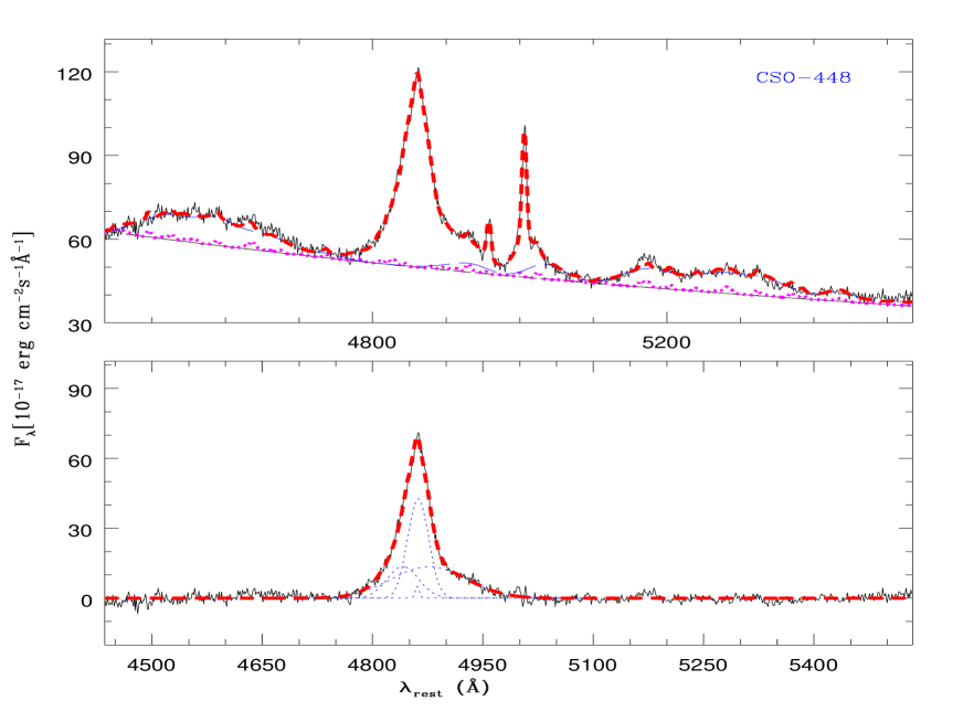
Figure 1: The best fit to the H$\beta$ emission line of the SDSS spectra of the QSO CSO 448. Upper panel: complete spectrum fit (thick dashed/red) and components of the fit: power law continuum (thin dashed/black line), broad Fe ii  (dot-dashed/blue), narrow Fe ii  (dotted/magenta) lines. Lower panel: continuum, Fe ii  and metal line subtracted spectrum (solid/black) with the best fit total H$\beta$ profile (thick dashed/red) and H$\beta$  components (dotted/blue) lines. Note that the entire fit is performed simultaneously (not first continuum subtraction then H$\beta$ fit) but these aspects are shown separately for the sake of clarity.

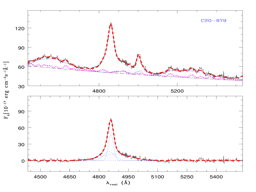
Figure 2: Same as Fig. 1 for CSO 879.

3 Line analysis through simultaneous spectral fitting

The spectra were first corrected for Galactic extinction using the extinction map of Schlegel et al. (1998) and the reddening curve of Fitzpatrick (1999). Then they were transformed into the rest frame using the redshift given in the header of the SDSS spectra.

In order to have accurate measurements of spectral properties such as the EWs and FWHMs of emission lines, one has to carefully take into account the contribution from continuum as well as from Fe ii emission multiplets. The common practice was to first fit and subtract the AGN continuum and then the Fe ii emission (e.g., Boroson & Green 1992; Marziani et al. 2003) and finally the other emission lines. The other possibility is to fit simultaneously the continuum and the Fe ii emission multiplets and other emission lines (e.g., Dong et al. 2008, 2009a). Unfortunately, for the optical spectra of most of RQQSOs in our sample, fitting the continuum and the Fe ii emission is very complicated because: (i) there are essentially no emission-line free regions where the continuum can be determined (Vanden Berk et al. 2001); (ii) the prominence of Fe ii features and their blending with the H$\beta$ and Mg ii lines; (iii) the H$\beta$ line is highly blended with the O iii$\lambda\lambda$4959,5007 lines. As a result, we have opted to carry out simultaneous fits of continuum, Fe ii emission, H$\beta$ and Mg ii and all other metal emission lines present in the spectra.

For this purpose we follow the following procedure.

3.1 H$\beta$  region fit

For fitting the optical region comprising the H$\beta$ line, we consider the rest wavelength range between 4435 and 5535 Å. The continuum is modeled by a single power law, as since we limit ourselves to below 5600Å  there is no need of a double or broken power law fit (e.g, Dong et al. 2008). As the profile of the H$\beta$ line is rather complex, it is fitted with multiple (as many as four) Gaussians. As an initial guess we consider two narrow, one broad and one very broad components. To reduce the arbitrariness of the component fits and also to make the decomposition more physical, we have constrained the redshift and width of the two narrow components of H$\beta$ to be the same as those of the O iii$\lambda\lambda$4959,5007 lines. The line profile of O iii$\lambda$5007 (and hence of O iii$\lambda$4959 ) are modeled as double Gaussians, with one stronger narrow component with width less than 2000 km s${}^{-1}~{}$ and one weaker broader component with width less than 4000 km s${}^{-1}~{}$. However, if for some source spectra the second component is not statistically required, the procedure we use automatically drops it during the fit. So, basically we have only four free parameters for the width and redshift of O iii$\lambda\lambda$4959,5007 and narrow H$\beta$  components (two for redshift and two for width).

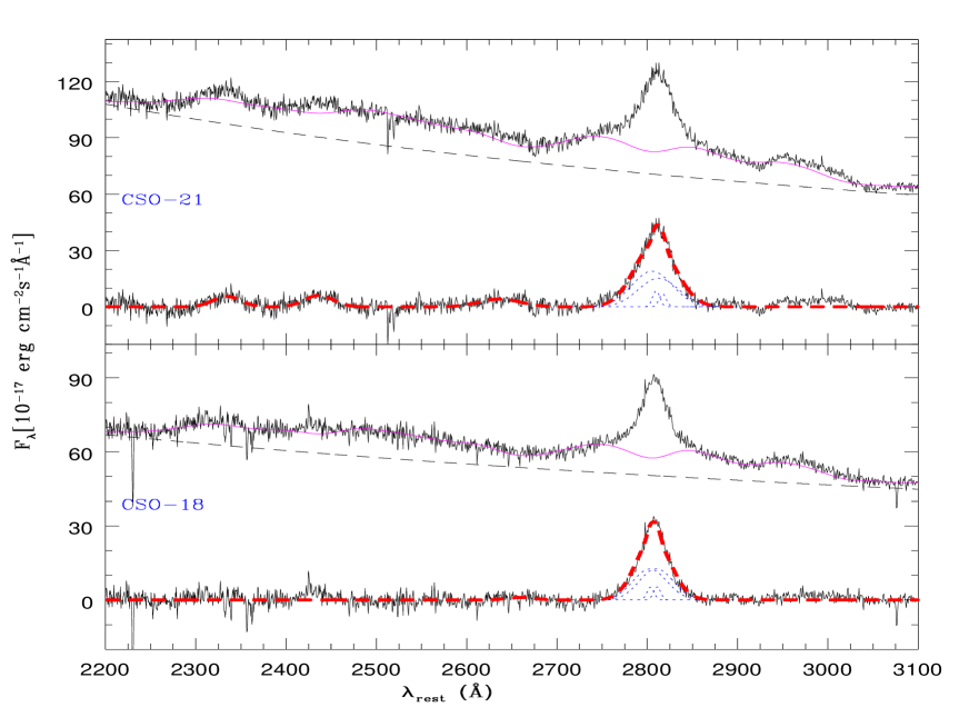
Figure 3: Mg ii emission line fits for two RQQSOs, CSO 21 and CSO 18. The upper plot in each panel shows the SDSS spectra and continuum as a dashed line with the best fit UV Fe ii  template as a solid (magenta) line. The lower plot in each panel show the continuum and Fe ii  subtracted spectrum (solid) the best fit Mg ii profile (thick dashed/red) and Mg ii$\lambda\lambda$2796,2803  components by (dotted/blue) lines. Note that the entire fits are performed simultaneously (not first continuum subtraction, then Mg ii fit) but are shown separately for the sake of clarity.

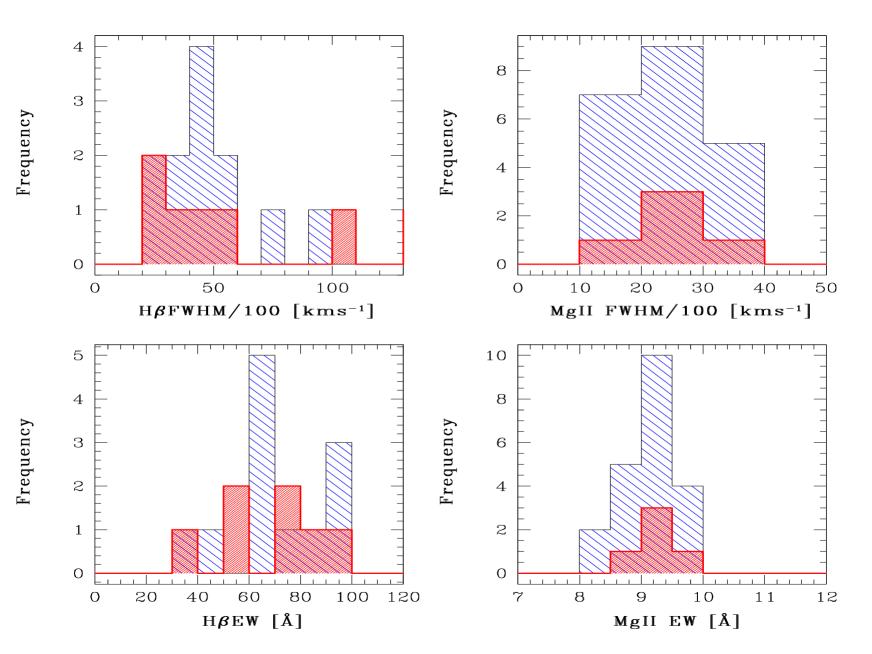
Figure 4: Histograms of FWHM and rest frame equivalent width (EW) based on best fits of H$\beta$ and Mg ii lines. The shaded regions correspond to sources with confirmed optical microvariability while the non-shaded regions are for those sources for which optical microvariability is not detected.

The optical Fe ii  emission is modeled with two separate sets of templates in analytical forms similar to those used by Dong et al. (2008). One template is for the broad-line system and the other for the narrow-line system, and we assume the form $C(\lambda)=c_{b}C_{b}(\lambda)+c_{n}C_{n}(\lambda)$, where $C_{b}(\lambda)$ represents the broad Fe ii lines and $C_{n}(\lambda)$ the narrow Fe ii lines, with the relative intensities fixed at those of I ZW 1, as given in Tables A.1 and A.2 of Véron-Cetty, Joly & Véron (2004). The redshift of the broad Fe ii lines and the H$\beta$  component is fitted as a free parameter while their widths are kept the same, with a constraint that they should be larger than 1000 km s${}^{-1}~{}$; this width is used for estimating the BH masses. Similarly for the narrow Fe ii line the redshift is fitted as a free parameter but the width is kept the same as that of the stronger narrow O iii$\lambda$5007 component. The fourth (very broad) H$\beta$ component, if required for the fit, is subject only to the constraint that its width should be more than 1000 km s${}^{-1}~{}$. The emission lines other than Fe ii and O iii$\lambda\lambda$4959,5007 (see Table 2 in Vanden Berk et al. 2001), are modeled with single Gaussians. The final fit is achieved by simultaneously varying all the free parameters to minimize the $\chi^{2}~{}$ value until the reduced $\chi^{2}_{r}$ is $\approx 1$. Samples of our spectral fitting in the optical region are given for H$\beta$ in Fig. 1 and Fig. 2. The values for FWHM and EW (both the broad component, EW_B, and total, EW_all) for the H$\beta$ lines are given in Table 2.

Table 2: Results of the H$\beta$ line analyses

QSO Name	z	$\frac{L(5100\AA)}{10^{44}\rm erg~{}s^{-1}}$	FWHM(km s-1)	log($\frac{M_{bh}}{M_{\odot}}$)	$\frac{L_{bol}}{L_{edd}}$	EWB(Å)	EWall(Å)
CSO 174	0.653	18.41	7034.92	9.24	0.07	10.42	$95.31\pm 0.98$
CSO 179	0.782	52.71	5039.39	9.18	0.24	47.80	$87.87\pm 1.21$
CSO 448	0.317	7.45	3133.75	8.34	0.23	14.42	$78.97\pm 0.66$
CSO 879	0.551	27.24	4072.64	8.85	0.26	21.36	$91.02\pm 0.67$
Mrk 1014	0.163	3.77	2393.82	7.96	0.28	30.69	$53.53\pm 0.51$
PG 0832$+$251	0.331	13.89	5059.36	8.89	0.12	20.72	$84.59\pm 0.55$
PG 0923$+$201	0.192	8.85	10461.15	9.42	0.02	48.81	$75.77\pm 0.49$
PG 0931$+$437	0.458	31.42	9537.59	9.62	0.05	11.47	$68.42\pm 0.52$
PG 1049$-$005	0.359	24.17	5193.56	9.03	0.15	22.16	$76.06\pm 0.40$
PG 1259$+$593	0.474	42.13	2922.88	8.65	0.63	4.33	$41.06\pm 0.50$
PG 1307$+$085	0.154	5.22	4080.08	8.49	0.11	62.77	$99.83\pm 0.54$
PG 1309$+$355	0.183	10.98	4326.57	8.70	0.15	20.86	$35.27\pm 0.46$
PG 1444$+$407	0.268	10.15	3528.12	8.51	0.21	8.26	$66.90\pm 0.50$
Q 1252$+$0200	0.344	16.62	23694.59	10.27	0.01	26.78	$90.09\pm 0.54$
TON 52	0.434	16.68	2724.97	8.39	0.46	11.90	$38.78\pm 0.69$
US 1867	0.514	25.11	2837.29	8.52	0.52	33.89	$68.80\pm 0.46$
US 3150	0.469	14.44	3402.68	8.55	0.27	14.78	$68.28\pm 0.67$
US 3472	0.532	25.48	4587.36	8.94	0.20	14.30	$69.93\pm 0.64$
US 995	0.227	3.90	4509.77	8.51	0.08	46.58	$51.95\pm 0.58$

Table 3: Results of the Mg ii line analyses

QSO Name	z	$\frac{L(3000\AA)}{10^{44}\rm erg~{}s^{-1}}$	FWHM(kms-1)	Log($\frac{M_{bh}}{M_{\odot}}$)	Log($\frac{M_{bh}}{M_{\odot}}$)	$\frac{L_{bol}}{L_{edd}}$	EWB(Å)	EWall(Å)
CSO 18	1.300	139.87	$2728.10\pm 0.49$	8.71	9.25	0.32	20.28	$22.09\pm 0.37$
CSO 21	1.190	151.63	$3244.49\pm 0.82$	8.88	9.41	0.24	22.80	$24.65\pm 0.33$
CSO 233	2.030	220.37	$1670.96\pm 0.95$	8.40	8.92	1.08	17.60	$17.60\pm 0.84$
CSO 879	0.549	44.02	$1548.88\pm 0.50$	7.90(8.85)	8.50	0.56	10.47	$14.96\pm 0.33$
PG 0935$+$416	1.966	711.91	$2518.34\pm 1.19$	9.08	9.53	0.86	4.68	$5.00\pm 0.34$
PG 0946$+$301	1.220	355.37	$2216.44\pm 0.37$	8.78	9.27	0.78	13.62	$14.80\pm 0.27$
PG 1206$+$459	1.155	607.67	$2441.60\pm 0.76$	9.01	9.47	0.84	12.30	$13.46\pm 0.21$
PG 1248$+$401	1.032	254.23	$2337.98\pm 0.28$	8.73	9.24	0.59	16.82	$18.84\pm 0.30$
PG 1254$+$047	1.018	231.12	$3603.36\pm 0.57$	9.08	9.60	0.24	15.65	$18.63\pm 0.28$
PG 1259$+$593	0.472	76.12	$2417.71\pm 0.65$	8.44(8.65)	9.01	0.30	8.77	$12.71\pm 0.28$
PG 1338$+$416	1.204	249.35	$3062.60\pm 0.85$	8.96	9.47	0.34	13.22	$16.08\pm 0.29$
PG 1630$+$377	1.478	612.30	$2793.42\pm 1.91$	9.13	9.59	0.65	12.12	$13.45\pm 0.26$
Q 1628.5$+$3808	1.461	193.09	$2167.82\pm 0.58$	8.59	9.12	0.60	16.54	$16.54\pm 0.37$
Q J0751$+$2919	0.912	347.62	$2432.96\pm 0.37$	8.85	9.34	0.64	14.79	$15.98\pm 0.25$
UM 497	2.022	342.38	$1901.77\pm 0.56$	8.63	9.13	1.04	22.83	$22.83\pm 0.46$
US 1420	1.473	199.32	$1708.34\pm 0.45$	8.40	8.92	0.98	7.50	$10.76\pm 0.33$
US 1443	1.564	302.09	$2589.39\pm 0.61$	8.87	9.37	0.53	14.10	$14.10\pm 0.30$
US 1498	1.406	162.70	$1844.98\pm 0.29$	8.41	8.94	0.76	11.73	$12.87\pm 0.34$
US 1867	0.513	39.58	$1745.21\pm 0.39$	7.98(8.52)	8.58	0.42	13.12	$16.87\pm 0.24$
US 3150	0.467	22.81	$1467.23\pm 1.09$	7.68(8.55)	8.31	0.45	8.84	$13.46\pm 0.39$
US 3472	0.532	45.26	$2234.99\pm 0.39$	8.23(8.94)	8.83	0.27	15.13	$18.94\pm 0.32$
TON 52	0.434	28.10	$1739.86\pm 0.78$	7.88(8.39)	8.51	0.36	17.31	$17.31\pm 0.49$
CSO 174	0.653	36.73	$3564.17\pm 1.06$	8.58(9.24)	9.19	0.10	32.41	$36.94\pm 0.36$
TON 34	1.925	1761.85	$3006.16\pm 0.62$	9.47	9.88	0.94	10.77	$14.04\pm 0.28$
CSO 179	0.782	95.95	$2691.86\pm 0.28$	8.59(9.18)	9.15	0.28	20.44	$25.62\pm 0.33$
PG 1522$+$101	1.328	765.86	$3437.96\pm 0.90$	9.37	9.82	0.48	15.66	$16.13\pm 0.25$

3.2 Mg ii  doublet region fit

For fitting the Mg ii doublet region, we consider a rest wavelength range between 2200 and 3200 Å. The continuum in this region is modeled by a power law, i.e., $a_{1}\lambda^{-\alpha}$. For fitting the Mg ii  doublet we have tried both Gaussians and truncated 5-parameter Gauss-Hermite series (Salviander et al. 2007; Dong et al. 2009a). In Gaussian profile fits, our initial guess consists of two Gaussian components for each line of the Mg ii  doublet; however, whenever the second component is not statistically required the procedure automatically drops it during the fit. Only two cases where single components fits were found to be sufficient were detected (UM 479 and US 1443). To test for any overfitting caused by assuming two components, we also forced our procedure to fit only single components; however, in doing so for all other sources, a very good fit is found neither for the wings of the lines nor for their central narrow cores. The truncated 5-parameter Gauss-Hermite series was also tried, but the fits in this case also were not as good as those from the two component Gaussian profile model, so our final analyses employ that fitting approach.

In our two component Gaussian profile fits, the redshift and width of each component (narrow/broad) of Mg ii$\lambda$2796  were tied to the respective components of the Mg ii$\lambda$2803 line. In addition, we have constrained the width of narrow component to be smaller than 1000 km s${}^{-1}~{}$  and the width of the broader Mg ii component to be same as width of UV Fe ii  emission line in the region (UV Fe ii ). We used an UV Fe ii template generated by Tsuzuki et al. (2006), basically from the measurements of I ZW 1, which also employ calculations with the CLOUDY photoionization code (Ferland et al. 1998). This template is scaled and convolved to the FWHM value equivalent to the broad components of Mg ii  by taking into account the FWHM of the I ZW 1 template. The best fit value of the broad component of Mg ii  obtained in this way is finally used in our calculation of BH mass. The emission lines other than Fe ii lines identified from the composite SDSS QSO spectrum (see Table 2 in Vanden Berk et al. 2001), are modeled with single Gaussians. The final fit is achieved by varying all the free parameters simultaneously by minimizing the $\chi^{2}~{}$ value, until the reduced $\chi^{2}_{r}$ is $\approx 1$. Demonstrations of our spectral fitting in the UV region are given in Fig. 3, and values for FWMHs and EWs are given in Table 3.

3.3 Optical microvariability and spectral properties

Among the 19 sources for which we have spectral coverage of the H$\beta$ line, optical microvariability is shown by 7 of them while the other 12 have not been seen to show this property (Carini et al. 2007). Similarly, among the 26 sources with spectral coverage of Mg ii doublet, only 5 show optical microvariability but the other 21 do not.

We have used our best fit values of FWHM and EW to search for any correlation between them and optical microvariability. The median value of total rest frame EW of the H$\beta$ line (i.e., the sum of the EWs of all fitted components) for 12 sources without optical microvariability is found to be $\sim 69$ Å. Its value for the 7 sources having optical microvariability is $\sim 79$ Å. This seems to be contrary to the expectation based on a blazar component model of microvariability for RQQSOs, which would predict smaller EW values for variable sources, due to dilution of emission line strength by jet components (Czerny et al. 2008). However, it should be noted that observed H$\beta$ profiles certainly require multiple components to fit them. Therefore, if optical microvariability is a phenomenon related to the central AGN engine, then it is presumably better to do such a comparison only using the broad component of the H$\beta$ line (Section 3.1). This is because the clouds responsible for this broad component are clearly in the sphere of influence of the massive BH, while the other components may not be. The median value of rest frame EW of this component for objects showing any optical microvariability is $26.8$ Å  and for objects without optical microvariability it is $20.8$ Å, which is again contrary to the expectation based on a blazar component model of optical microvariability. The corresponding values of median FWHM of these broad components for sources with and without microvariability are somewhat different, at $4509$ km s^-1 and $4326$ km s^-1, respectively.

Similar to what we did with the H$\beta$ line, we have also used our Mg ii spectral fits to look for any correlation with microvariability. The median value of rest frame EW of broad Mg ii doublet components (with width tied to the UV Fe ii template width) is found to be $9.15$ Å  for the five sources with optical microvariability and $9.24$ Å  for the 21 sources without any confirmed microvariability. These values are essentially identical, and so again do not support the simple blazar component model for microvariability in RQQSOs. The corresponding values of median FWHM for sources with and without microvariability are $2432$ km s ^-1 and $2447$ km s^-1, respectively, and so are indistinguishable.

In Fig. 4 we show the histograms of our FWHM and rest frame EW values based on our best fits for H$\beta$ and Mg ii lines. The shaded and non-shaded regions correspond respectively to sources with and without confirmed optical microvariability. As the figure shows, the distributions of sources with and without microvariability are on the whole quite similar, though there seems to be a hint that the median EW width of the H$\beta$ line might be larger for sources with optical microvariability compared to those without optical microvariability. To quantify this posibility we performed Kolmogorov-Smirnov tests on all the distributions shown in Fig. 4. The probabilities that the sources with and without confirmed optical microvariability are drawn from similar distributions are: 0.613 for $\rm H\beta(\rm EW)$; 0.664 for $\rm Mg~{}II(\rm EW)$; 0.792 for $\rm H\beta(\rm FWHM)$ and 0.995 for $\rm Mg~{}II(\rm FWHM)$. As these null probabilities are all high our data samples do not establish or support any relation of FWHM or EW with the optical microvariability properties. The lack of a difference in the EW values does not support simple models in which the microvariability arises from jets.

4 Black Hole Mass Measurements

The strong M_BH-$\sigma$ correlation between supermassive black hole (SMBH) mass and the velocity dispersion of the surrounding spheroidal stellar system (e.g., Tremaine et al. 2002) have shown that black hole (BH) assembly is intimately related to the bulge properties of its host galaxy. This paradigm of “BH–galaxy co-evolution” boosted the efforts to measure BH masses over a wide range (e.g., Richstone et al. 1998; Nelson 2000; Bower et al. 2000). However, one cannot obtain BH mass estimates from either stellar or gas dynamics, based upon traditional methods, beyond $\sim$100 Mpc, due to the difficulty in resolving the BH sphere of influence. For these more distant sources the only viable way to probe BH masses is through their AGN activity.

The reverberation mapping technique (e.g., Blandford & McKee 1982; Peterson 1993) is the most direct method to probe gas dynamics on spatial scales close to the BH in AGN, but the required long-duration spectroscopic monitoring campaigns currently preclude the method from being applied to large numbers of objects. Because the time-lags involved grow linearly with the SMBH mass, only relatively nearby Seyfert galaxies with modest values of $M_{\rm BH}$ have been studied in this fashion. Therefore for any large statistical studies one has to rely on the more indirect technique of virial single-epoch methods, which were pioneered by Dibai (1980) and shown to be consistent with reverberation mapping masses (e.g., Bochkarev & Gaskell 2009). These measurements make use of the widths of emission lines such as H$\beta$ , Mg ii or C iv in conjunction with the bolometric luminosity (e.g., Vestergaard & Peterson 2006). This method relies upon the FWHM indicating the typical velocities of clouds bound to the BH and the assumption that the mean distances, $r$, of the clouds emitting particular lines are determined by their ionization potentials, and thus scale with the ionizing continuum, $L$, of the QSO. We have used our H$\beta$ or Mg ii FWHM measurements to compute the BH mass of RQQSOs in our sample, as such estimates will also impose important constraints in studies trying to understand the nature of RQQSOs (e.g., Czerny et al. 2008).

Vestergaard & Peterson (2006) presented improved empirical relationships useful for estimating the central BH mass based on FWHMs of emission lines such as H$\beta$ , Mg ii and C iv . We used their following scaling relation to estimate the BH masses based on H$\beta$  lines (Vestergaard et al. 2006, their Eq. 5)

$$\log\,M_{\rm BH}(\rm H\beta)=\log\,\left[\left(\frac{\rm FWHM(H\beta)}{1000~{}km~{}s^{-1}}\right)^{2}\right]$$ (1)

$$\mbox{}+(6.91\pm 0.02)+\log\,\left(\frac{\lambda\it L_{\lambda}{\rm(5100\,\AA)}}{10^{44}\rm erg~{}s^{-1}}\right)^{0.50\pm 0.06}~{},$$

where $L_{\lambda}{\rm(5100\,\AA)}$ is the monochromatic luminosity at 5100 Å, which we have computed from the best fit power-law continuum, $a_{1}\lambda^{-\alpha}$, in our simultaneous fit of the whole spectral region (see Section 3.1).

As is evident from this equation, careful measurements of the FWHM of emission lines are crucial for good BH mass estimations. So it is very important to decompose the lines into broad and narrow components, since the former are much more likely to be in the BH sphere of influence, while the later are contributed from the much more distant narrow line region under the dynamical influence of the galaxy’s stellar component. Therefore, as described in Section 3.1, we have constrained the narrow component’s profile to be linked to the O iii$\lambda\lambda$4959,5007 line profile while the broad component’s profile is associated with the broad Fe ii emission multiplet. We have modeled the whole Fe ii emission multiplet by also decomposing it into broad and narrow component contributions. This aspect of the fitting has been largely ignored in almost all previous BH mass estimation studies until recent efforts by Dong et al. (2008, 2009a). So in the above Eq. 1 the FWHM we used, from among our Gaussian de-composition of H$\beta$  line (Section 3), is the one with its width tied with the width of the broad Fe ii  emission line, after correcting for instrumental broadening. The result of our analysis using H$\beta$ lines is summarized in Table 2.

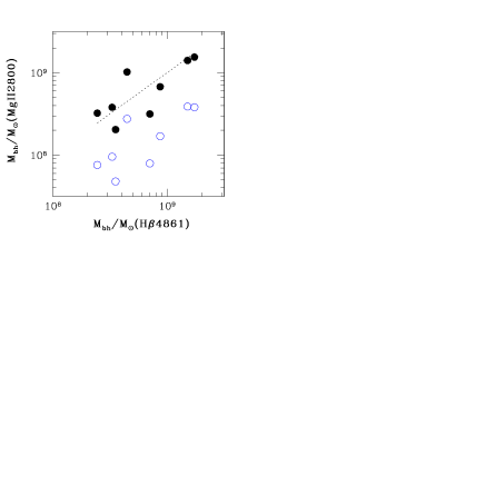
Figure 5: Comparison of BH masses estimated using H$\beta$ and Mg ii lines for the eight sources for which spectra cover both H$\beta$ and Mg ii lines. The Mg ii based BH masses using Eq. 2 (McLure & Dunlop 2004) are shown by hollow circles, while those based on Eq. 3 (Dietrich et al. 2009) are shown by filled circles. The dotted line shows equal BH masses estimated using H$\beta$ and Mg ii lines.

To estimate black hole masses based on Mg ii , we initially adopted the calibrations in McLure & Dunlop (2004), i.e.,

$$\log\,M_{\rm BH}(\rm Mg~{}II)=(0.62\pm 0.14)\log\left(\frac{\lambda\it L_{\lambda}\rm(3000\,\AA)}{10^{44}\rm erg~{}s^{-1}}\right)$$ (2)

$$\mbox{}+2\log\left(\frac{\rm FWHM(Mg~{}II)}{\rm km~{}s^{-1}}\right)+0.505~{},$$

where the monochromatic luminosity at 3000 Å  has been computed from our power-law fit of the continuum and the FWHM used is the broad component of our double Gaussian decomposition model, after correcting for the instrumental broadening. The result of our Mg ii  analysis for black hole mass based on the McLure & Dunlop (2004) scaling relation is summarized in Column 5 of Table 3.

In our sample eight QSO spectra cover both Mg ii and H$\beta$ lines, which allow us to compare whether or not the black hole masses estimated with them are consistent with one another. As can be noted from column 5 of Table 3, where BH mass estimates based on H$\beta$ lines are in parentheses, the differences can be even as large as 0.95 dex (e.g., CSO 879, Fig. 2). Also, we note that in all eight cases the Mg ii based mass estimate is smaller than the one based on the H$\beta$ line. One possible reason could be the uncertainty in the slope, $\beta$ of the $r$–$L$ relation; from Eq. 2, $\beta=0.62\pm 0.14$, so the nominal uncertainty is $\sim 25$ per cent. Recent studies on the $r$–$L$ relation also indicate that the slope of the radius–luminosity relation is close to $\beta=0.5$, consistent with basic predictions of photoionization models (e.g., Davidson & Netzer 1979; Osterbrock & Ferland 2005). The presence of steeper slopes in some analyses appear to be caused by not correcting for contributions of the host galaxy to the continuum luminosity (Bentz et al. 2006; Bentz et al. 2009). Dietrich et al. (2009) have addressed this problem by assuming the slope of the $r$–$L$ relation to be 0.5, as seems to hold for the H$\beta$ line, and they then calculated the average scaling constant $D$; following their Eq. (6), viz,

$$M_{bh}(H\beta) = M_{bh}(\rm Mg~{}II)=D\,\biggl{(}{\lambda L_{\lambda}(3000)\over{10^{46}{\rm erg\,s}^{-1}}}\biggr{)}^{0.5}\,$$ (3)

$$\biggl{(}{FWHM({\rm MgII}\lambda 2800)\over{1000\,{\rm km\,s}^{-1}}}\biggr{)}^{2}M_{\odot}\ ~{},$$

where the M_bh(H$\beta$) values were computed from their near-infrared spectra and the FWHM(MgII$\lambda$ 2800) values came from their optical spectra. They find $D=(2.0\pm 0.5)\times 10^{8}\,M_{\odot}$. Using this empirical constant $D$ in Eq.  3, we recalculated the Mg ii -based BH masses; the results are given in the sixth column of Table 3. As can be noted from columns (5) and (6) and illustrated in Fig. 5, the discrepancy between the masses from the two lines for the cases where both can be evaluated is reduced, and ranges from 0.05 to 0.36 dex, which is within the expected systematic uncertainty of black hole masses (around a factor of 4) based on single epoch measurements (Vestergaard & Peterson 2006). These consistent BH mass estimates range from $\sim 10^{8}$ to $>10^{9}~{}M_{\odot}$ for our sample. We note that the prescriptions we have adopted are not unique and that several other prescriptions for black hole masses in terms of virial parameters obtained from H$\alpha$ as well as H$\beta$ and Mg ii also have been considered. These have been recently summarized by McGill et al. (2008) who show that the level of agreement we have obtained can be improved upon somewhat with the consideration of a larger number of AGN.

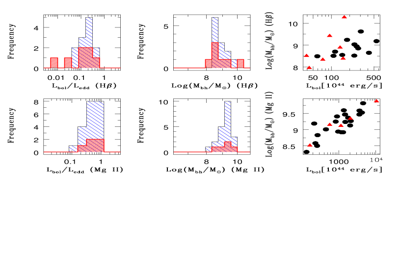
Figure 6: The upper left and middle panels show the histograms of Eddington ratio $L_{bol}/L_{edd}$ and ${\rm log}(M_{bh}/M_{\odot})$ based on the H$\beta$ line, while the corresponding bottom panels show the results based on the Mg ii line. The shaded regions correspond to sources with confirmed optical microvariability while the non-shaded regions are for those sources for which optical microvariability is not detected. The right upper and bottom panels respectively show plots of ${\rm log}(M_{bh}/M_{\odot})$ versus $L_{bol}$. Triangles and circles respectively show sources with and without confirmed optical microvariability.

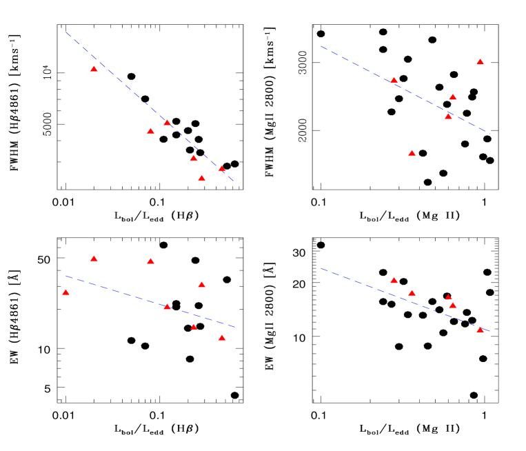
Figure 7: Observed variation of FWHM (upper) and EW (lower) with Eddington ratio ($\ell={\rm L}_{bol}/{\rm L}_{edd}$) based on both H$\beta$ (left) and Mg ii (right) lines. Triangles and circles respectively show sources with and without confirmed optical microvariability. The dashed lines show the linear regression fits treating $\ell$ as the independent variable. The correlations of both FWHM and EW with $\ell$, suggest that the Eddington ratio is one of the fundamental parameters responsible for some AGN properties.

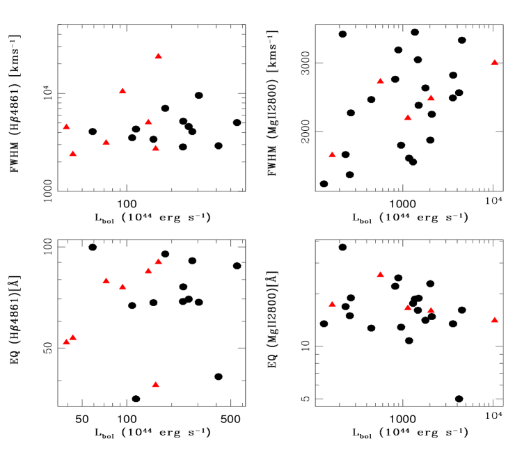
Figure 8: As in Fig. 7 with $L_{\rm bol}$ as the independent variable. This panel indicates that most of the sources with optical microvariability are of low luminosities.

Table 4: BH growth time estimates (in units of Gyr) from the H$\beta$ line analysis

object	z	$L_{bol}$/$L_{edd}$ = 1.0			$L_{bol}$/$L_{edd}$ obs.			age of the
		$M_{bh}$(seed)			$M_{bh}$(seed)			Universe
		$10\,M_{\odot}$	$10^{3}\,M_{\odot}$	$10^{5}\,M_{\odot}$	$10\,M_{\odot}$	$10^{3}\,M_{\odot}$	$10^{5}\,M_{\odot}$	[$10^{9}$ yr]
CSO 174	0.653	0.83	0.63	0.43	11.81	8.94	6.07	7.44
CSO 179	0.782	0.82	0.62	0.42	3.42	2.58	1.75	6.73
CSO 448	0.317	0.74	0.54	0.33	3.20	2.33	1.46	9.89
CSO 879	0.551	0.79	0.59	0.39	3.03	2.26	1.49	8.08
Mrk 1014	0.163	0.70	0.50	0.30	2.49	1.78	1.06	11.43
PG 0832$+$251	0.331	0.79	0.59	0.39	6.59	4.92	3.25	9.77
PG 0923$+$201	0.192	0.84	0.64	0.44	42.22	32.19	22.16	11.12
PG 0931$+$437	0.458	0.86	0.66	0.46	17.29	13.28	9.27	8.73
PG 1049$-$005	0.359	0.81	0.60	0.40	5.37	4.03	2.69	9.52
PG 1259$+$593	0.474	0.77	0.57	0.37	1.22	0.90	0.58	8.62
PG 1307$+$085	0.154	0.75	0.55	0.35	6.83	5.01	3.18	11.53
PG 1309$+$355	0.183	0.77	0.57	0.37	5.15	3.81	2.47	11.22
PG 1444$+$407	0.268	0.75	0.55	0.35	3.59	2.63	1.68	10.35
Q 1252$+$0200	0.344	0.93	0.73	0.53	92.97	72.91	52.85	9.66
TON 52	0.434	0.74	0.54	0.34	1.61	1.18	0.74	8.91
US 1867	0.514	0.75	0.55	0.35	1.45	1.06	0.68	8.33
US 3150	0.469	0.76	0.56	0.36	2.80	2.06	1.32	8.65
US 3472	0.532	0.80	0.60	0.40	3.98	2.98	1.98	8.20
US 995	0.227	0.75	0.55	0.35	9.41	6.91	4.40	10.76

Table 5: BH growth time estimates (in units of Gyr) from the Mg ii line analysis

object	z	$L_{bol}$/$L_{edd}$ = 1.0			$L_{bol}$/$L_{edd}$ obs.			age of the
		$M_{bh}$(seed)			$M_{bh}$(seed)			Universe
		$10\,M_{\odot}$	$10^{3}\,M_{\odot}$	$10^{5}\,M_{\odot}$	$10\,M_{\odot}$	$10^{3}\,M_{\odot}$	$10^{5}\,M_{\odot}$	[$10^{9}$ yr]
CSO 18	1.300	0.83	0.63	0.43	2.59	1.96	1.33	4.73
CSO 21	1.190	0.84	0.64	0.44	3.51	2.68	1.84	5.07
CSO 233	2.030	0.79	0.59	0.39	0.74	0.55	0.36	3.18
CSO 879	0.549	0.75	0.55	0.35	1.34	0.98	0.63	8.09
PG 0935$+$416	1.966	0.86	0.65	0.45	0.99	0.76	0.53	3.28
PG 0946$+$301	1.220	0.83	0.63	0.43	1.06	0.81	0.55	4.97
PG 1206$+$459	1.155	0.85	0.65	0.45	1.01	0.77	0.53	5.18
PG 1248$+$401	1.032	0.83	0.63	0.43	1.40	1.06	0.72	5.63
PG 1254$+$047	1.018	0.86	0.66	0.46	3.59	2.76	1.92	5.68
PG 1259$+$593	0.472	0.80	0.60	0.40	2.68	2.01	1.34	8.63
PG 1338$+$416	1.204	0.85	0.65	0.45	2.50	1.91	1.32	5.02
PG 1630$+$377	1.478	0.86	0.66	0.46	1.33	1.02	0.71	4.25
Q 1628.5$+$3808	1.461	0.81	0.61	0.41	1.36	1.02	0.69	4.30
Q J0751$+$2919	0.912	0.84	0.64	0.44	1.31	0.99	0.68	6.12
UM 497	2.022	0.82	0.61	0.41	0.78	0.59	0.40	3.19
US 1420	1.473	0.79	0.59	0.39	0.81	0.61	0.40	4.27
US 1443	1.564	0.84	0.64	0.44	1.58	1.21	0.83	4.05
US 1498	1.406	0.80	0.60	0.40	1.05	0.78	0.52	4.44
US 1867	0.513	0.76	0.56	0.36	1.81	1.33	0.85	8.33
US 3150	0.467	0.73	0.53	0.33	1.63	1.18	0.74	8.67
US 3472	0.532	0.79	0.58	0.38	2.91	2.17	1.42	8.20
TON 52	0.434	0.75	0.55	0.35	2.09	1.53	0.98	8.92
CSO 174	0.653	0.82	0.62	0.42	8.21	6.21	4.20	7.43
TON 34	1.925	0.89	0.69	0.49	0.95	0.73	0.52	3.35
CSO 179	0.782	0.82	0.62	0.42	2.92	2.20	1.49	6.73
PG 1522$+$101	1.328	0.88	0.68	0.48	1.84	1.42	1.01	4.65

5 Eddington ratios and black hole growth times

We have also estimated the Eddington ratio $\ell\equiv L_{bol}/L_{edd}$, where $L_{bol}$ is taken as $5.9\times\lambda L_{\lambda}$(3000Å) and $9.8\times\lambda L_{\lambda}$(5100Å) for Mg ii and H$\beta$ , respectively (McLure & Dunlop 2004), and $L_{edd}=1.45\times 10^{38}(M_{bh}/M_{\odot})\rm erg~{}s^{-1}$, assuming a mixture of hydrogen and helium so the mean molecular weight is $\mu=1.15$. The results are given in Fig. 6 which shows that distributions of sources showing and not showing optical microvariability are not significantly different with respect to either BH mass or $\ell$.

To test the reasonableness of estimated Eddington ratios, we also computed black hole growth times to compare them with the age of the Universe (at the time the QSO is observed), by using the following equation (Dietrich et al. 2009),

$$M_{bh}(t_{obs})=M_{bh}^{seed}(t_{0})\,{\rm exp}\biggl{(}\ell\,{(1-\epsilon)\over\epsilon}\,{\tau\over t_{edd}}\biggr{)}~{},$$ (4)

where $\tau=t_{obs}-t_{0}$ is the time elapsed since the initial time, $t_{0}$, to the observed time, $t_{obs}$; $M_{bh}^{seed}$ is the seed BH mass; $\epsilon$ is the efficiency of converting mass to energy in the accretion flow, and $t_{edd}$ is the Eddington time scale, with $t_{edd}=\sigma_{T}c/4\pi Gm_{p}=3.92\times 10^{8}$ yr (Rees 1984). We used Eq. 4 to derive the times, $\tau$, necessary to accumulate the BH masses listed in Tables 2 and 3, for seed black holes with masses of $M_{bh}^{seed}=10M_{\odot}$, $10^{3}M_{\odot}$, and $10^{5}M_{\odot}$, respectively. Two cases are considered: (i) BHs are accreting at the Eddington-limit, i.e., $\ell$ = L_bol/L_edd = 1.0 and the efficiency of converting mass into energy is $\epsilon=0.1$; (ii) BHs are accreting with our observed Eddington ratios and $\epsilon=0.1$. These results are summarized in Tables 4 and  5.

In Fig. 7 we show the observed variations of FWHM and EW with $\ell$ based on both H$\beta$ and Mg ii lines. There appear to be linear relations of both FWHM and EW with $\ell$ in these log-log plots. For the FWHM plots this is unsurprising since the BH masses are proportional to $L_{edd}$. To quantify any such linear relations for the EW plots we perform linear regressions, treating $\ell$ as the independent variable, and find

$$\rm logEW(H\beta)=(1.12\pm 0.14)+(-0.22\pm 0.15)\rm log\ell,$$

$$\rm logEW(\rm Mg~{}II)=(1.04\pm 0.05)+(-0.34\pm 0.12)\rm log\ell.$$ (5)

Here the errors on the fit parameters are purely statistical. We have calculated the Spearman rank correlations of logEW with log$\ell$, and found the correlation coefficient for r${}_{s}(H\beta)=-0.22$, with null probability $p_{null}=0.35$, and so only a possible weak correlation is present. Whereas r${}_{s}(\rm Mg~{}II)=-0.52$, with $p_{null}=0.01$ and so this negative correlation is significant.

6 Discussion and Conclusions

Several recent papers have used the very large numbers of quasars discovered by modern surveys to estimate their BH masses using virial approaches (e.g., Shen et al. 2008; Fine et al. 2008; Vestergaard & Osmer 2009). The large numbers of quasars whose spectra are fit in these particular papers (between 1100 and almost 57,700) have allowed for very important new conclusions to be drawn about quasar demography. Shen et al. (2008) have found that the line widths of H$\beta$ and Mg ii follow lognormal distributions with very weak dependencies on redshift and luminosity. Their comparison of BH masses of radio-loud quasars (RLQSOs) and BALs with those of “ordinary” quasars (RQQSOs) shows that the mean of virial masses of RLQSOs is 0.12 dex larger than that of ordinary quasars, while that of BALs is indistinguishable from that of ordinary quasars. Fine et al. (2008) used Mg ii lines to estimate BH masses, and found that the scatter in measured BH masses is luminosity dependent, showing less scatter for more luminous objects. Vestergaard & Osmer (2009) have studied the mass functions of BH masses at different redshifts, and found evidence for cosmic downsizing in their cosmic space density distributions.

The sample we have considered is much smaller, but each member has been carefully selected to be among the special group of RQQSOs and Seyfert galaxies already examined for optical microvariability (e.g., Carini et al. 2007). This criterion demands that modest aperture (usually 1–2 m) telescopes can make precise photometric measurements in just a few minutes, and so limits the members to the rare QSOs with bright apparent magnitudes (usually $m_{V}<17.5$). In addition, special care was taken in the fitting of the line profiles as discussed in Sections 3.1 and 3.2.

As the precision of CCD based differential photometry has typically improved to better than 0.01 mag for these measurements made in a few minutes, the question as to the presence of microvariability in RQQSOs has been clearly settled in the affirmative (Gopal-Krishna et al. 2000, 2003; Stalin et al. 2004a,b; Gupta & Joshi 2005; Carini et al. 2007; Gupta & Yuan 2009; Ramírez et al. 2009). However these papers find that the duty cycle (DC), or fraction of nights such behavior is detected, is low, roughly 10–20%, for RQQSOs observed for reasonably long periods (4 hours or more) during a night. On the other hand, blazars show much more rapid variability, with DCs for such monitoring periods around 50–60% and when observed for $>6$ hours the blazar DCs rise to 60–85% (e.g., Carini 1990; Sagar et al. 2004; Gupta & Joshi 2005). The difference in microvariabilty amplitudes and DCs between RQQSOs and blazars can be easily understood if all the fluctuations arise from a jet very close to the central engine, but that jet only escapes that region and emits significant radio power for RL objects (e.g., Gopal-Krishna et al. 2003; Gopal-Krishna, Mangalam & Wiita 2008). And most RLQSOs that are not blazars would only have modest (if any) Doppler boosting, so that they also have DCs comparable to those of RQQSOs, as found in the samples of Stalin et al. (2005) and Ramírez et al. (2009), or at a level between those of RQQSOs and blazars (35–40%, in the sample of Gupta & Joshi 2005), is not surprising. Only recently has a decent sized sample of radio intermediate quasars (RIQs), defined as those relatively rare objects with radio to optical flux ratios in the regime between those that are truly radio quiet and those normally defined as RLQSOs, been targeted for microvariability monitoring (Goyal et al. 2009); their key result is that the RIQs also probably have a DC $\leq$ 20%. Therefore they are not likely to be beamed versions of RQQSOs as has been frequently suggested (Goyal et al. 2009).

We conclude that there may be a weak negative correlation between H$\beta$ EW and the Eddington ratio, $\ell$, but there is a significant one between the Mg ii EW and $\ell$ (Fig. 7; Section 5). This latter point has been made independently and more firmly by Dong et al. (2009b) using a larger sample drawn from SDSS. We can also see from Fig. 7 that there is a decline in FWHM with $\ell$; this is unsurprising since the BH masses are proportional to $L_{edd}$. We see from Fig. 8 that there is a tendency for sources with detectable optical microvariability to have somewhat lower luminosities than those with no such detections. This is interesting, and should be confirmed by examining larger samples. But it is not surprising, as regardless of whether the microvariability arises in accretion discs or jets, more massive BHs have naturally longer characteristic timescales that will presumably make any variations harder to detect over the course of a single night.

We also find that the BH masses estimated from the FWHMs of both the H$\beta$ and Mg ii lines are reasonable, in that growth to their estimated masses from even small seed BHs is easily possible within the age of the Universe at their observed redshift if the mean $\ell$ values are close to unity (Tables 4 and 5). This remains true for the great majority of RQQSOs if the value of $\ell$ we compute from the current continuum flux was constant until the time we observe them; however, this assumption does not work for 4 out of the 19 QSOs with H$\beta$ lines. It is also problematical for 1 out of the 26 QSOs with Mg ii lines (i.e., CSO 174, which is also among the difficult set of 4 using H$\beta$ profiles).

We find no difference between the EWs (of both the H$\beta$ or Mg ii lines) and the presence or absence of radio emission in those QSOs (Figs. 4 and 7). As discussed in the introduction, if much of the optical emission in RLQSOs comes from a jet, then we would expect the EWs of the RLQSO sources to be significantly lower than those of the RQQSOs, and if anything, they are slightly higher in our sample. This result does not support the hypothesis (e.g., Czerny et al. 2008) that RQQSOs possess jets that are producing rapid variations. Instead it may indicate that variations involving the accretion disc (e.g., Wiita 2006) play an important role here.

Improvements to our results could be obtained through extensive searches for INOV in a larger sample of RQQSOs. It should be useful to divide the sample of sources based on their EWs as available from SDSS, or otherwise uniformly obtained, spectra. Such samples could be divided into three classes based on EW of H$\beta$ , e.g., EW$<$40Å, 40Å$\leq$ EW $<$ 80Å  and EW $\geq$ 80Å. Such samples should be made as homogeneous as possible on the basis of apparent magnitudes, $z$ and M_V. With such larger and homogeneous samples, the absence of a correlation between EW and DC of INOV, as found here in our modest sample, could be confirmed or shown to be unlikely.

References

- Abazajian et al. (2009) Abazajian K. N., Adelman-McCarthy J. K. Agüeros, M. A., et al., 2009, ApJS, 182, 543
- Bentz, M.C., (2006) Bentz M. C., Peterson B. M., Pogge R. W., Vestergaard M., Onken C. A., 2006, ApJ, 644, 133
- Bentz, M.C., (2009) Bentz M. C., Peterson B. M., Netzer H., Pogge R. W., Vestergaard M., 2009, ApJ, 697, 160
- Blandford & McKee. (1982) Blanford R. D., McKee C. F., 1982, ApJ, 255, 419
- Bochkarev & Gaskell (2009) Bochkarev N. G., Gaskell, C. M., 2009, Astron. Lett., 35, 287
- Boroson & Green (1992) Boroson T. A., Green R. F., 1992, ApJS, 80, 109
- Bower et al. (2000) Bower G. A., Green R. F., Quillen, A. C., et al., 2000, ApJ, 534, 189
- Carini, M.T. 1 (990) Carini M. T., 1990, PhD Thesis, Georgia State Univ.
- Carini et al. (2007) Carini M. T., Nobel J. C., Taylor R., Culler, R., AJ, 133, 303
- Czerny et al., (2008) Czerny B., Siemiginowska A., Janiuk A., Gupta A. C., 2008, MNRAS, 386, 1557
- Davidson & Netzer (1979) Davidson K., Netzer H., 1979, Rev. Mod. Phys., 51, 715
- Dibai (1992) Dibai É. A., 1980, Sov. Astron., 24, 389
- Dietrich et al. (2009) Dietrich M., Mathur S., Grupe D., Komossa S., 2009, ApJ, 696, 1998
- Dong et al. (2008) Dong X.-B., Wang T.-G., Wang J.-G., Yuan W., Zhou H., Dai H., Zhang K., 2008, MNRAS, 383, 581
- Dong et al. (2009a) Dong X.-B, Wang J.-G, Wang T.-G, Wang H., Fan X., Zhou H., Yuan, W., 2009a, arXiv:0903.5020
- Dong et al. (2009b) Dong X.-B., Wang T.-G., Wang J.-G., Fan X., Wang H., Zhou H., Yuan W., 2009b, ApJL, 703, L1
- Ferland et al. (1998) Ferland G. J., Korista K. T., Verner D. A., Ferguson J. W., Kingdon J. B., Verner, E. M., 1998, PASP, 110, 761
- Fine et al. (2008) Fine S., Croom S. M., Hopkins P. F., et al., 2008, MNRAS, 390, 1413
- Fitzpatrick (1999) Fitzpatrick E. L., 1999, PASP, 111, 63
- Forster K. et al. (2001) Forster K., Green P. J., Aldcroft T. L., Vestergaard M., Foltz C. B., Hewett P. C., 2001, ApJS, 134, 35
- Gaskell C. M., (2006) Gaskell C. M., 2006, in Gaskell C. M., McHardy I. M., Peterson B. M., Sergeev S. G., eds, ASP Conf. Ser. Vol. 360, AGN Variability from Xrays to Radio Waves. Astron. Soc. Pac., San Francisco, p. 111
- Gopal-Krishna et al. (1993) Gopal-Krishna, Wiita P. J., Altieri B., 1993, A&A, 271, 89
- Gopal-Krishna et al. (2000) Gopal-Krishna, Gupta A. C., Sagar R., Wiita P. J., Chaubey U. S., Stalin C. S., 2000, MNRAS, 314, 815
- Gopal-Krishna et al. (2003) Gopal-Krishna, Stalin C. S., Sagar R., Wiita P. J., 2003, ApJ, 586, L25
- Gopal-Krishna et al. (2008) Gopal-Krishna, Mangalam A., Wiita P. J., 2008, ApJ, 680, L13
- Goyal et al. (2009) Goyal A., Gopal-Krishna, Joshi S., Sagar R., Wiita P. J., Anupama G. C., Sahu D. K., 2010, MNRAS, 401, 2622
- Gupta al. al (2005) Gupta A. C., Joshi U. C. 2005, A&A, 440, 855
- Gupta al. al (2009) Gupta A. C., Yuan W., 2009, New Astron., 14, 88
- Kelly et al. (2009) Kelly B. C., Bechtold J., Siemiginowska A., 2009, ApJ, 698, 895
- Marchã et al. (1996) Marchã M. J. M., Browne I. W. A., Impey C. D., Smith P. S., 1996 MNRAS, 281, 425
- Marscher et al. (1992) Marscher A. P., Gear W. K., Travis J. P., in E. Valtaoja & M. Valtonen, eds, Variability of Blazars. Cambridge Univ. Press, Cambridge, p. 85
- Marziani et al. (2003) Marziani P., Sulentic J. W., Zamanov R., Calvani M., Dultzin-Hacyan D., Bachev R., Zwitter, T., 2003, ApJS, 145, 199
- McGill et al. (2008) McGill K. L., Woo J.-H., Treu T., Malkan M. A., 2008, ApJ, 673, 703
- McLure & Dunlop (2004) McLure R. J., Dunlop J. S., 2004, MNRAS, 352, 1390
- Miller H. R. et al. (1989) Miller H. R., Carini M. T., Goodrich B. D., 1989, Nat, 377, 627
- Nelson (2000) Nelson C. H., 2000, ApJ, 544, 91
- Osterbrock & Ferland (2005) Osterbrock D. E., Ferland G. J., 2005, Astrophysics of Gaseous Nebulae and Active Galactic Nuclei, 2nd edition, University Science Books, Sausalito
- Peterson (1993) Peterson B. M., 1993, PASP, 105, 247
- Ramírez et al. (2009) Ramírez A., de Diego J. A., Dultzin D., Gonzalez-Perez J.-N., 2009, AJ, 138, 991
- Rees (1984) Rees M. J., 1984, ARA&A, 22, 471
- Richstone, D. et al. (1998) Richstone D., Ajhar E. A., Bender R., et al., 1998, Nature, 395, 14
- Rokaki et al. (1993) Rokaki E., Collin-Souffrin S., Magnan C., 1993, A&A, 272, 8
- Sagar et al. (2004) Sagar R., Stalin C. S., Gopal-Krishna, Wiita P. J., 2004, MNRAS, 348, 176
- Salviander et al. (2007) Salviander S., Shields G. A., Gebhardt K., Bonning E. W., 2007, ApJ, 662, 131
- Schlegel, Finkbeiner, & Davis (1998) Schlegel D. J., Finkbeiner D. P., Davis M., 1998, ApJ, 500, 525
- Shen et al. (2008) Shen Y., Greene J. E., Strauss M. A., Richards G. T., Schneider D. P., ApJ, 680, 169
- Stalin et al. (2004a) Stalin C. S., Gopal-Krishna, Sagar R., Wiita P. J., 2004a, JApA, 25, 1
- Stalin et al. (2004b) Stalin C. S., Gopal-Krishna, Sagar R., Wiita P. J., 2004b, MNRAS, 350, 175
- Stalin et al. (2005) Stalin C. S., Gupta A. C., Gopal-Krishna, Wiita P. J., Sagar R., 2005, MNRAS, 356, 607
- Stickel et al. (1991) Stickel M., Padovani P., Urry C. M., Fried J. W., Kühr H., 1991, ApJ, 374, 431
- Tremaine et al. (2002) Tremaine S., Gebhardt K., Bender R., et al., 2002, ApJ, 574, 740
- Tsuzuki et al. (2006) Tsuzuki Y., Kawara K., Yoshii Y., Oyabu S., Tanabé T., Matsuoka Y. 2006, ApJ, 650, 57
- Vanden Berk et al. (2001) Vanden Berk D. E., Richards G. T., Bauer, A., et al., 2001, AJ, 122, 549
- Véron-Cetty et al. (2004) Véron-Cetty M.-P., Joly M., Véron P., 2004, A&A, 417, 515
- Véron-Cetty & Véron (2006) Véron-Cetty M.-P., Véron P., 2006, A&A, 455, 773
- Vestergaard & Osmer (2009) Vestergaard M., Osmer P. S., 2009, ApJ, 699, 800