On the geometry of Julia sets

Abstract.

We show that the Julia set of quadratic maps with parameters in hyperbolic components of the Mandelbrot set is given by a transseries formula, rapidly convergent at any repelling periodic point.

Up to conformal transformations, we obtain $J$ from a smoother curve of lower Hausdorff dimension, by replacing pieces of the more regular curve by increasingly rescaled elementary “bricks” obtained from the transseries expression. Self-similarity of $J$, up to conformal transformation, is manifest in the formulas.

The Hausdorff dimension of $J$ is estimated by the transseries formula. The analysis extends to polynomial maps.

1. Introduction

Iterations of maps are among the simplest mathematical models of chaos. The understanding of their behavior and of the associated fractal Julia sets (cf. §1.1 for a brief overview of relevant notions) has progressed tremendously since the pioneering work of Fatou and Julia (cf. [9]–[11]). The subject triggered the development of powerful new mathematical tools. In spite of a vast literature and of a century of fundamental advances, many important problems are still not completely understood, even in the case of quadratic maps, see e.g. [13].

As discussed in [2], a “major open question about fractal sets is to provide quantities which describe their complexity. The Hausdorff dimension is the most well known such quantity, but it does not tell much about the fine structure of the set. Two sets with the same Hausdorff dimension may indeed look very different (computer pictures of these sets, although very approximate, may reveal such differences).“

A central goal of this paper is to provide a detailed geometric analysis of local properties of Julia sets of polynomial maps.

It will be apparent from the proof that the method and many results apply to polynomials of any order. However, we will frequently use for illustration purposes the quadratic map $z\mapsto z^{2}+c$, or equivalently after a linear change of variable, $x\mapsto P(x)=\lambda x(1-x)$, $c=\lambda/2-\lambda^{2}/4$ (note the symmetry $\lambda\to 2-\lambda$). The associated map iteration is

$$x_{n+1}=P(x_{n})$$ (1)

Our analysis applies to the hyperbolic components of the Mandelbrot set of the iteration, see §1.1. Let $\varphi$ be the Bötcher map of $P$ (with the definition (4) below), analytic in the punctured unit disk $\mathbb{D}\setminus\{0\}$; then $J=\varphi(\partial\mathbb{D})$.

Let $p_{0}=\varphi(e^{2\pi it_{0}})$ be any periodic point on $J$. We show that for $z\in\mathbb{D}$ near $e^{2\pi it_{0}}$, $\varphi$ is given by an entire function of $s^{b}\omega(\ln s)$ where $s=-\ln(e^{-2\pi it_{0}}z)$ (clearly $s\to 0$ as $p_{0}$ is approached). Here $b$ has a simple formula and $\omega$ is a real analytic periodic function.

In particular, at any such $p_{0}$, the local shape of $J$ is, to leading order, the image of the segment $[-\epsilon,\epsilon]$ under a map of the form $Az^{b}$. The averaged value $b_{E}$ of $b$ (over all periodic points) and the Hausdorff dimension of $J$, $D_{H}$, satisfy $D_{H}\geq 1/\mathrm{Re}\,b_{E}$. Up to conformal transformations, $J$ is obtained from a curve of higher regularity and lower Hausdorff dimension than $J$, by replacing pieces of the more regular curve by increasingly rescaled basic “bricks” obtained from the transseries expression. This is analogous to the way elementary fractals such as the Koch snowflake are obtained. We present figures representing $J$ for various parameters in this constructive way.

1.1. Notation and summary of known results

We use standard terminology from the theory of iterations of holomorphic maps. If $f$ is an entire map, the set of points in $\mathbb{C}$ for which the iterates $\{f_{n}\}_{n\in\mathbb{N}}$ form a normal family in the sense of Montel is called the Fatou set $\mathcal{F}$ of $f$ while the Julia set $J$ is $\mathbb{C}\setminus\mathcal{F}$. For instance, if $f=P$ ($P$ being the quadratic map above) and $|\lambda|<1$, the Fatou set has two connected components, $\mathcal{F}_{\infty}=\{z_{0}:|P_{n}(z_{0})|\to\infty\text{ as }n\to\infty\}$ and $\mathcal{F}_{0}=\{z_{0}:|P_{n}(z_{0})|\to 0\text{ as }n\to\infty\}$ where

$$P_{n}=P^{\circ n}$$

is the $n$-th self-composition of $P$. The Julia set in this example is $\overline{\mathcal{F}_{0}}\cap\overline{\mathcal{F}_{\infty}}$, a Jordan curve.

The substitution $x=-y^{-1}$ transforms (1) into

$$y_{n+1}=\frac{y_{n}^{2}}{\lambda(1+y_{n})}=f(y_{n})$$ (2)

By Bötcher’s theorem (for (1) we give a self contained proof in §3.5), there exists a unique map $F$, analytic near zero, with $F(0)=0$, $F^{\prime}(0)=\lambda^{-1}$ so that $(F\circ f\circ F^{-1})(x)=x^{2}$. Its inverse, $G$, used in [8], conjugates (2) to the canonical map $z_{n+1}=z_{n}^{2}$, and it can be checked that

$$G(z)^{2}=\lambda G(z^{2})(1+G(z));\ \ G(0)=0,\ G^{\prime}(0)=\lambda$$ (3)

Equivalently (with $\varphi=1/G$) there exists a unique map $\varphi$ analytic in $\mathbb{D}\setminus\{0\}$

$$P(\varphi(z))=\varphi(z^{2});\ \ \ z\in\mathbb{D}\setminus\{0\};\ \ \lim_{z\to 0}z\varphi(z)=1/\lambda$$ (4)

We list some further definitions and known facts that we use; see, e.g., [1, 5, 13].

Remark 1.

1. $J$ is the closure of the set of repelling periodic points.

2. For polynomial maps, and more generally, for entire maps, $J$ is the boundary of the set of points which converge to infinity under the iteration.

3. For general polynomial maps, if the maximal disk of analyticity of $G$ (where now $1/G(z^{n})=P_{n}(1/G(z))$) is the unit disk $\mathbb{D}_{1}$, then $G$ maps $\mathbb{D}_{1}$ biholomorphically onto the immediate basin $\mathcal{A}_{0}$ of zero. If on the contrary the maximal disk is $\mathbb{D}_{r},\,r<1$, then there is at least one other critical point in $\mathcal{A}_{0}$, lying in $G(\partial\mathbb{D}_{r})=J_{y}$, the Julia set of (2), see [13] p.93.

4. If $r=1$, it follows that $G(\partial\mathbb{D}_{1})=J_{y}$.

5. For the iteration $t_{n+1}=t_{n}^{2}+c$, the Mandelbrot set is defined as (see e.g. [5])

   $$\mathcal{M}=\{c:t_{n}\text{ bounded }\text{ if }t_{0}=0\}$$ (5)

   If $c\in\mathcal{M}$, then clearly $y_{n}$ in (2) are bounded away from zero.

6. $\mathcal{M}$ is a compact set; it coincides with the set of $c$ for which $J$ is connected. The main cardioid $\mathcal{H}=\{(2e^{it}-e^{2it})/4:t\in[0,2\pi)\}$ is contained in $\mathcal{M}$; see [5]. This means $\{\lambda:|\lambda|<1\}$ corresponds to the interior of $\mathcal{M}$. We have $|\lambda|=1\Rightarrow c\in\partial\mathcal{M}\subset\mathcal{M}$.

   Assume now that $c\in\mathcal{M}$ and $\lambda\neq 0$. Then,

7. The function $\varphi$ extends analytically to $\mathbb{D}$.

8. ([8] p. 121) If $z$ approaches a rational angle, $e^{2\pi it},\ t\in\mathbb{Q}$, then the limit

   $$L_{t}=\lim_{\rho\to 1}\varphi\left(\rho e^{2\pi it}\right)\ \ \text{exists.}$$ (6)

9. ([17]) A quadratic map has at most one non-repelling periodic orbit.

10. For every $\lambda$ such that the corresponding $c$ is in $\mathcal{M}$, and any $t\in\mathbb{Q}$, the limit

    $$\varphi\left(ze^{2\pi it}\right)\to L_{t}\ \text{as}\ z\to 1\ \text{nontangentially}\$$ (7)

    exists. (See also [12].) This follows immediately from (6), the boundedness of $\varphi$ and the Sectorial Limit Theorem, see [4], p. 23, Theorem 5.4.

11. In any hyperbolic component of $\mathcal{M}$ (components of $\mathcal{M}$ corresponding to (unique) attracting cycles), the points $z\in$ fix $P_{n}$ on the corresponding Julia set have the property $|P^{\prime}_{n}(z)|>1$ and $\varphi$ is continuous in $\overline{\mathbb{D}}$.

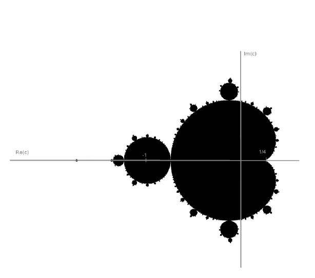
Figure 1. The Madelbrot set.

2. Main results

2.1. Expansions at the fixed points

Assume that $c$ is in the interior of $\mathcal{M}$ and let

$$s=-\ln(e^{-2\pi it}z)$$

Note that $s\to 0$ as $z\to e^{2\pi it}$. We can of course restrict the analysis to $t\in[0,1)$, and from this point on we shall assume this is the case. As is well known, if $t=p/q$ with odd $q$, then the binary expansion of $t$ is periodic; in general it is eventually periodic.

Theorem 1.

(i) Let $t=p/q$ with odd $q$, take $N$ between $1$ and $q-1$ so that $2^{N}t=t\mod 1$, and let $M=2^{N}$. There is a $\ln M$-periodic function $\omega$, analytic in the strip $\{\zeta:|\mathrm{Im}\zeta|<\pi/2\}$ and an entire function $g$ so that $g(0)=0,g^{\prime}(0)=1$ and

$$\varphi(z)=L_{t}+g\left(s^{b}\omega(\ln s)\right)$$ (8)

$$b=b(L_{t})=\frac{\ln(P^{\prime}_{N}(L_{t}))}{N\ln 2}$$ (9)

for $|\arg\ln s|\leq\pi/2$ and where $P_{N}(L_{t})=L_{t}$.

(ii) If $\lambda\notin\{0,2\}$, then the lines $\mathrm{Im}z=\pm\pi/2$ are natural boundaries for $\omega$. In particular, $\omega$ is a nontrivial function for these $\lambda$.

(iii) If $t=p/(2^{M}q)$ with $q$ odd and $M>0$, and $z=z_{1}e^{2\pi it}$, then we have $z^{2^{M}}=z_{1}^{2^{M}}e^{2\pi it^{\prime}}$ where $t^{\prime}$ is as in (i). We have

$$\varphi(z)=L_{t}+\frac{g\left({s^{\prime}}^{b}\omega(\ln s^{\prime})\right)}{P^{\prime}_{M}(L_{t})}+g^{2}\left({s^{\prime}}^{b}\omega(\ln s^{\prime})\right)F_{1}\left(g\left({s^{\prime}}^{b}\omega(\ln s^{\prime})\right)\right)$$ (10)

where $s^{\prime}$ is as in (i) with $t$ replaced by $t^{\prime}$ and $F_{1}$ is an algebraic function, analytic at the origin.

Corollary 1.

It follows from Theorem 1 (i) that the Fourier coefficients $c_{k}$ of $\omega$ decrease roughly like $d^{k}$, with $d=e^{-2\pi^{2}/\ln M}$. Since $2\pi^{2}/\ln 2\approx 28.5$, $\omega$ can often be numerically replaced, with good accuracy, by a constant.

Corollary 2.

The function $\varphi$ has the following convergent transseries expansion near $z=e^{2\pi it}$ ($t=p/q$, $q$ odd.)

$$\varphi(z)=L_{t}+\sum_{n=1}^{\infty}a_{n}\left(s^{b}\sum_{k=-\infty}^{\infty}c_{k}s^{2k\pi i/\ln{M}}\right)^{n}\\ =L_{t}+\sum_{n=0}^{\infty}\sum_{k=-\infty}^{\infty}A_{n,k}(-\ln(e^{-2\pi it}z))^{nb+2k\pi i/\ln{M}}$$ (11)

where $a_{n}$ decrease faster than geometrically and $A_{n,k}$ decrease faster than $\epsilon^{n}d^{k}$, with $d$ as in Corollary 1 and $\epsilon>0$ arbitrary. A similar result holds for $t=p/(2^{m}q)$.

Proof.

A straightforward calculation using Theorem 1, where

$$g(z)=\sum_{n=1}^{\infty}a_{n}z^{n},\;\omega(t)=\sum_{k=-\infty}^{\infty}c_{k}e^{2k\pi it/\ln M}$$

The rate of decay of the coefficients follows immediately from Theorem 1 (i) and Corollary 1. ∎

We note that, in some cases including the interior of the main cardioid of $\mathcal{M}$, the expansion (11) converges on $\partial\mathbb{D}$ as well (though, of course, slower). This is a consequence of the Dirichlet-Dini theorem and the Hölder continuity of $\omega$ in the closure of its analyticity domain (by (12)) and of the Hölder continuity of $\varphi$, shown, e.g., in [3]).

Note 3.

Self-similarity is manifest in (8). Indeed, since $\omega$ is periodic and $g^{\prime}\neq 0$ (see the proof of Lemma 15 below), $\omega$ can be determined from any sufficiently large piece of $J$. Then, (8) shows that, up to conformal transformations and rescaling, this piece is reproduced in a neighborhood of any periodic point.

We see that

$${\omega}(\ln s)=s^{-b}g^{-1}({\varphi}(z)-L_{t})$$ (12)

Note 4 (Evaluating the transseries coefficients).

There are many ways to obtain the coefficients in (11). A natural way is the following. (i) First, the series of $g$ is found by simply iterating the contractive map in Lemma 15 below; the series for $g^{-1}$ is calculated analogously.

(ii) The relation (12), together with the truncated Laurent series of $\varphi$, can be used over one period of $\omega$ inside the domain of convergence of the series of $g^{-1}$, to determine a sufficient number of Fourier coefficients of $\omega$. The numerically optimal period depends of course on the value of $c$.

The accuracy of (11) increases as the boundary point is approached.

Note 5.

The list below gives $q$ (in brackets), together with the period of $1/q$ in base $2$ (underbraces).

$$\underbrace{[3]}_{2},\underbrace{[7]}_{3},\underbrace{[5,15]}_{4},\underbrace{[31]}_{5},\underbrace{[9,21,63]}_{6},\underbrace{[127]}_{7},\underbrace{[17,51,85,255]}_{8},...$$ (13)

where more than one denominator indicates that $2^{N}-1$ is not prime, and for each prime factor of $2^{N}-1$ we obviously get different periodic orbits.

Example 6.

For $\lambda=0.9$ we get the following rounded off values of $b$ indexed by $N=2,3,...$ (note that cusps are generated iff $\mathrm{Re}b<1$):

$$[0.13],[1.16],[1.08-0.145i,1.08+0.15i],[0.98-0.19i,0.98+0.19i,1.09],\\ [0.904-0.21i,0.904+0.21i,1.04-0.069i,1.04+0.069i,1.12-0.089i,1.12+0.089i]...$$ (14)

with $\beta_{t}:=\mathrm{Re}\,b_{t}$ clearly given by

$$[0.13],[1.16],[1.08],[0.98,1.09],[0.904,1.04,1.12]...$$ (15)

Note 7.

Along the periodic orbit $L_{t},P(L_{t}),...,P_{N-1}(L_{t})$ we have $P^{\prime}_{N}=const$ and $b=const$. Indeed, this follows from the fact that $P^{\prime}_{N}(L_{t})=P^{\prime}(L_{t})\cdots P^{\prime}_{N-1}(L_{t})$ is invariant under cyclic permutations.

Part of Theorem 1 follows from the more general result below. It is convenient to map the problem to the right half plane, by writing $\varphi(z_{0}e^{-t})=\varphi(z_{0})+F_{0}(t)$.

Assumption 1.

(i) Let $A$ and $F_{0}$ be analytic in the right half plane $\mathbb{H}$ and assume that for some $n>1$ it satisfies the functional relation

$$F_{0}(nx)=A(F_{0}(x))$$ (16)

(ii) Assume that $F_{0}\to 0$ along any curve lying in a Stolz angle in $\mathbb{H}$ (nontangential limit, see [4]; this is the case for instance if $F_{0}$ is bounded near zero and $F_{0}\to 0$ along some particular nontangential ray).

(iii) Assume that $|w|>1$, where $w=A^{\prime}(0)$ (note that, by (i) and (ii), $A(0)=0$).

Theorem 2.

Under the assumptions above, there exists a unique analytic function $g$, with $g(0)=0$ and $g^{\prime}(0)=1$, and a multiplicatively periodic function $h$: $h(nx)=h(x)$, analytic in $\mathbb{H}$ so that, for sufficiently small $x$, $F_{0}$ is of the form (see (9))

$$F_{0}(x)=g\left(x^{\log_{n}w}h(x)\right)$$ (17)

Moreover, if $A$ is an entire function then $g$ is also an entire function, and the above expression is valid for all $x\in\mathbb{H}$.

Note 8 (Connection between transseries and local angles).

We see, using Theorem 1 (i), that in a neighborhood of a point $t$ of period $M=2^{N}$, $J$ is the image of a small arc of a circle, or equivalently of a segment $[-\epsilon,\epsilon]$ under a transformation of the form $\zeta\mapsto\zeta^{\beta+i\mathrm{Im}b}F(\zeta)$ ($\beta=\mathrm{Re}\,\,b$) with $F$ multiplicatively periodic. In an averaged sense (over many periods), or of course if $\mathrm{Im}\,b=0$ and $F$ is a constant, $\beta$ is the cusp at $L$; in general, the shape is a spiral.

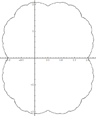
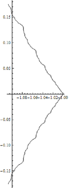
Figure 2. The Julia set for $\lambda=0.5$ (left figure), plotted by combining rescaled “bricks”. The “brick” (right): the local shape obtained from transseries expansion at $1$ .

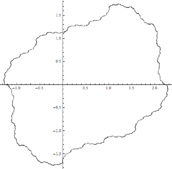
Figure 3. The Julia set for $\lambda=0.5i$, obtained from the transseries as Fig. 2.

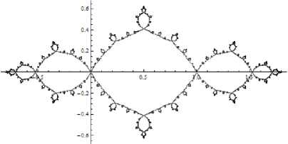
Figure 4. The Julia set for $\lambda=-1.25$, obtained from the transseries as Fig. 2.

2.1.1. The average branching

The critical point is outside $J$ (this is easy to show; see also the proof of Proposition 13). By continuity, zero is outside $P^{\prime}(J)$; by the argument principle, $\mathrm{Im}\ln(P^{\prime}(J))$ is bounded by $2\pi$ and $P^{\prime}(\varphi(e^{2\pi ix}))$ is bounded below and continuous. Using Proposition 13 and the continuity of $\varphi$ on $\partial\mathbb{D}$ we see that the following holds.

Corollary 9.

The average $b$,

$$b_{E}=\int_{0}^{1}\ln P^{\prime}(\varphi(e^{2\pi ix}))dx$$ (18)

with the natural branch of the log, is well defined.

Let $\beta_{E}=\mathrm{Re}\,\,b_{E}$.

2.2. Recursive construction of $J$

We say that a real number is “$(\epsilon,N,m)$-normal” on the initial set of $N$ bits if any block of bits of length $m$ of itself and its $m$ binary left shifts ($2x\mod 1$) appears with a relative frequency $1/Q$ within $\epsilon/Q$ errors, where $Q=2^{m}$. Consider the set of numbers $\mathcal{N}_{N,m,\epsilon}$ in $[0,1]$ which are not $(\epsilon,N,m)$-normal. The total measure Lebesgue measure of this set is estimated by, see §3.1,

$$\text{ meas }(\mathcal{N}_{N,m,\epsilon})\leq 2Qme^{-2N\epsilon^{2}/Q^{2}}$$ (19)

Consequently, for large $N_{0}$, we have

$$\text{ meas }\left(\mathcal{N}_{[N_{0}],m,\epsilon}\right)=O(Qme^{-2N_{0}\epsilon^{2}/Q^{2}})$$ (20)

where

$$\mathcal{N}_{[N_{0}],m,\epsilon}=\bigcup_{N\geq N_{0}}\mathcal{N}_{N,m,\epsilon}$$

The complement set $\mathcal{N}^{c}_{[N_{0}],m,\epsilon}$ can be obtained by excluding from $[0,1]$ intervals of size $2^{-Nm}$ around each binary rational with $Nm$ bits, which is not $(\epsilon,N,m)$-normal.

We denote as usual the Hausdorff dimension of $J$ by $D_{H}$.

Theorem 3.

Consider the curve $\tilde{J}$ obtained from $J$ by eliminating the binary rationals, modifying $\varphi$ in the following way. Define $\tilde{\varphi}=\varphi$ at all points $e^{2\pi iz}$ with $z\in\mathcal{N}^{c}_{[N_{0}],m,\epsilon}$. On the excluded intervals, $\tilde{\varphi}$ is simply defined by linear endpoint interpolation (cf. (50)). Let $\tilde{J}=\tilde{\varphi}(\partial\mathbb{D})$. Then, for any $\varepsilon>0$,

(i) The function $\tilde{\varphi}$ is Hölder continuous of exponent at least $\beta_{E}-\varepsilon$.

(ii) The Hausdorff dimension of the graph of $\tilde{\varphi}$ is less than $2-\beta_{E}+\varepsilon$. Here $\beta_{E}\geq 1/2$, see Note 14.

Note 10.

(i) The Hausdorff dimension of $\tilde{J}$ is lower than that of $J$. Indeed, this follows from $D_{H}\geq 1/\beta_{E}$, see (41) below, and

$$2-x<1/x,\ \ \ x\in(0,1)$$

(ii) Also, in large sections of the Mandelbrot set, including the main cardioid, the regularity of $\tilde{\varphi}$ is strictly better than that of $\varphi$.

In this sense, both the geometry (through regularity) and the Hausdorff dimension come from rational angles (more precisely, from the angles with non-normal distribution of digits in base $2$).

2.3. Hausdorff dimension versus angle distribution

Through the Ruelle-Bowen formula we see that $D_{H}$ can be seen as “inverse temperature” of the cusp system.

Notations (See the proof of Proposition 11 below for more details.) Let $\mu_{n}(\beta)=\text{prob}(\{z\in\text{fix}\,P_{n}:\beta(z)\leq\beta\}$, where the probability is taken with respect to the counting measure and let $F_{n}=\mu_{n}^{1/n}$. Let $w=P^{\prime}(0)$. Note that $F_{n}\in[0,1]$ are monotone (increasing) functions and right-continuous. Define $\overline{F}=\limsup_{n\to\infty}F_{n}$ and $\underline{F}=\liminf_{n\to\infty}F_{n}$, and denote, as usual for monotone functions, ${F_{+}(x)}=F(x+0)$ (the function $F_{+}$ is clearly right continuous.)

Define $\Phi=-\log_{2}F\in[0,\infty]$ (similarly, $\overline{\Phi}=-\log_{2}\overline{F}$ etc.) and let $\Phi^{\star}(t)=\max(ts-\Phi(s))$

Proposition 11.

We have

$$\overline{\Phi}_{+}^{\star}(-D_{H})=\underline{\Phi}_{+}^{\star}(-D_{H})=-1$$ (21)

Note 12.

Note also that all $b$ (cf. (9)) have nonnegative real part, since $|P^{\prime}(L_{t})|>1$ for $c$ in the hyperbolic components of $\mathcal{M}$, as seen next.

Proposition 13.

In any hyperbolic component of the Mandelbrot set there is a $\delta>0$ so that for any $\tau\in J$ we have $|P^{\prime}(\tau)|>\delta$.

Proof.

It is known [1] p. 194 that the immediate basin of any attracting cycle contains at least one critical point. Therefore, in the hyperbolic components of $\mathcal{M}$ the critical point cannot be on $J$. Since

$$P^{\prime}(\varphi(z))\varphi^{\prime}(z)=2z\varphi^{\prime}(z^{2})$$ (22)

the critical point cannot be inside either, since otherwise, solving (22) for $\varphi^{\prime}(z^{2})$ in terms of $\varphi^{\prime}(z)$, it is clear that $\varphi^{\prime}$ would vanish on a set with an accumulation point at $z=0$. Therefore $|P^{\prime}|>0$ on the continuous curve $J$. ∎

Theorem 4.

Assume $c$ is in a hyperbolic component of $\mathcal{M}$. (i) The Hausdorff dimension $D_{H}$ of $J$ satisfies

$$D_{H}\geq\beta_{E}^{-1}$$ (23)

(ii) On a set of full measure, $\varphi$ is Hölder continuous with exponent at least $\beta_{E}-\epsilon\geq 1/2-\epsilon$ for any $\epsilon>0$.

A direct and elementary proof of the theorem is given in §3.1.

Note 14.

Since $D_{H}\leq 2$, it follows that $\beta_{E}\geq 1/2$. (By a fundamental result of Shishikura [16], $D_{H}=2$ on the boundary of $\mathcal{M}$.)

3. Proofs and further results

Proof of Theorem 2.

Note that

$$A(y)=wy+y^{2}A_{0}(y)\ \ \text{where}\ \ A_{0}(y)=y^{-2}(A(y)-wy)\ \text{is a polynomial.}$$ (24)

We use an analytic solution of (16) to bring the equation of $F_{0}$ to a normal form.

Lemma 15 (Normal form coordinates).

There is a unique function $g$ analytic in a disk $\mathbb{D}_{\epsilon}$, such that $g(0)=0,g^{\prime}(0)=1$ (thus analytically invertible near zero) and

$$g(wy)=A(g(y))$$ (25)

Proof.

We write $g(y)=y+y^{2}g_{0}(y)$, $\alpha=1/w$ and get

$$g_{0}(y)=\alpha g_{0}(\alpha y)+\alpha^{2}(1+\alpha yg^{2}_{0}(\alpha y))^{2}A_{0}\left(\alpha y+\alpha^{2}y^{2}g_{0}(\alpha y)\right)$$ (26)

A straightforward verification shows that, for small $\epsilon$, (26) is contractive in the space of analytic functions in $\mathbb{D}_{\epsilon}$ in the ball $\|g_{0}\|\leq 2|A_{0}(0)|$, in the sup norm.

Define $H(x)=g^{-1}(F_{0}(x))$. (The definition is correct for small $x$ since $g$ is invertible for small argument, and $F_{0}$, by assumption is small). Obviously $H$ is analytic for small $x$. We see that

$$H(nx)=g^{-1}(A(F_{0}(x)))=g^{-1}(A(g(H(x))))=g^{-1}(g(wH(x)))=wH(x)$$ (27)

by (25). Taking $h(x)=x^{-\log_{n}w}H(x)$, the conclusion follows. Note that for any $r$, if $g$ is analytic in $\mathbb{D}_{r},$ then, by (25) and the monodromy theorem, $g$ is analytic in $\mathbb{D}_{|w|r}$ as long as $A$ is analytic in $\mathbb{D}_{r}$; since $r$ is arbitrary, it follows that $g$ is entire if $A$ is entire. In the same way, since $h(nx)=h(x)$, $h$ is analytic in $\mathbb{H}$. Note also that $g^{\prime}$ is never zero, since otherwise it would be zero on a set with an accumulation point at $0$, as it is seen by an argument similar to the one in the paragraph following (22). ∎

3.1. Probability distribution of angles

Consider the periodic points of period $mN$ ($m$ and $N$ conveniently large). These correspond, through $\varphi^{-1}$, to points of the form $z_{t}=e^{2\pi it}$ where $t$ has a periodic binary expansion of period $mN$.

Consider the orbit $z_{t},z_{t}^{2},...,z_{t}^{2^{Mn-1}}$ (by definition, $z_{t}^{2^{Mn}}=z_{t}$). We have, by formula (9), with $L_{t}=\varphi(z_{t})$,

$$b(L_{t})=N^{-1}m^{-1}\sum_{j=0}^{Nm-1}\log_{2}[P^{\prime}(\varphi(z_{t}^{2^{j}}))]$$ (28)

We analyze the deviations from uniform distribution of subsequences of $m$ consecutive bits in the block of length $Nm$. For this, it is convenient to rewrite the block of length $Nm$ in base $Q=2^{m}$, as now a block of length $N$ of $Q$-digits. Every binary $m$-block corresponds to a digit in $\{0,1,...,Q-1\}$ in base $Q$. To analyze the deviations, we rephrase the question as follows. Consider $N$ independent variables, $X_{1},...,X_{N}$ with values: $1$ with probability $1/Q$ if the digit $i$ equals $q$, and $0$ otherwise. The expectation $E(N^{-1}(X_{1}+\cdots+X_{N}))$ is clearly $1/Q$ and we have $\mathcal{P}(X_{i}-E(X_{i}))\in[-1/Q,1-1/Q]=1$ ($\mathcal{P}$ denotes probability). Then, with $S=X_{1}+\cdots+X_{N}$ we have, by Hoeffding’s inequality [7],

$$\mathcal{P}(|N^{-1}S-1/Q|>\epsilon/Q)\leq 2e^{-2N\epsilon^{2}/Q^{2}}$$ (29)

Using the elementary fact that $\mathcal{P}(A\vee B)\leq\mathcal{P}(A)+\mathcal{P}(B)$, we see that the probability of a block of length $N$ having the frequency of any digit departing $1/Q$ by $\epsilon/Q$ is at most

$$\mathcal{P}_{\epsilon}\leq 2Qe^{-2N\epsilon^{2}/Q^{2}}$$ (30)

We see that (28) involves shifts in base $2$ (and not in base $2^{m}$). The probability of a block of length $Nm$ in base $2$ having the frequency of any $m$-block in all its $m$ successive binary left-shifts ($x\to 2x\mod 1$) departing by $\epsilon/Q$ from its expected frequency of $1/Q$ is thus

$$\mathcal{P}\leq 2Qme^{-2N\epsilon^{2}/Q^{2}}$$ (31)

Therefore, the relative frequency of “$\epsilon$-normally distributed” $Nm$-periodic binary expansions with all $m$-size blocks of its binary shifts distributed within $\epsilon/Q$ of their expected average number is

$$\mathcal{P}\geq 1-2Qme^{-2N\epsilon^{2}/Q^{2}}$$ (32)

Let

$$b_{EQ}=Q^{-1}\sum_{j=0}^{Q-1}\log_{2}[P^{\prime}(\varphi(e^{2\pi ij/Q}))]$$ (33)

We take $f_{1}=\mathrm{Re}\log_{2}\left(P^{\prime}\circ\varphi\right)$ and $f_{2}=\mathrm{Im}\left(\log_{2}P^{\prime}\circ\varphi\right)$, and for a real function $f$ we write $f^{+}$ for its positive part and $f^{-}$ for its negative part. For any number $t$ which is $\epsilon$-normally distributed, the sequence $2^{j}t\mod 1$ will have $Nm(1/Q\pm\epsilon/Q)$ points in each interval of the form $[j/Q,j+1/Q]$. Therefore, taking the positive real part of the integrand in (28), we have the following bound for its contribution to the sum:

$$Q^{-1}(1-\epsilon)\sum_{j=0}^{Q-1}\min_{x\in[j/Q,(j+1)/Q]}f_{1}^{+}(e^{2\pi ix})\\ \leq Q^{-1}\sum_{j=0}^{Q-1}\rho(j/Q)\min_{x\in[j/Q,(j+1)/Q]}f_{1}^{+}(e^{2\pi ix})\leq N^{-1}m^{-1}\sum_{j=0}^{2^{Nm}-1}f_{1}^{+}(z^{2^{j}})$$ (34)

where $\rho(j/Q)$ is the frequency of $2^{j}t\mod 1$ belonging to $[j/Q,(j+1)/Q]$. Corresponding estimates hold with $\leq$ replaced by $\geq$ and $\min$ with $\max$. Since

$$Q^{-1}(1-\epsilon)\sum_{j=0}^{Q-1}\min_{x\in[j/Q,(j+1)/Q]}f_{1}^{+}(e^{2\pi ix})\to\int_{0}^{1}f_{1}^{+}(e^{2\pi ix})dx$$ (35)

as $Q\to\infty$ and $\epsilon\to 0$ (and similarly for $f_{1}^{-}$ and $f_{2}^{\pm}$), for any $\epsilon_{1}>0$ we can choose $Q$ large enough and and $\epsilon$ small enough so that on the set of blocks described above (31) we have

$$|b_{EQ}-b_{E}|<\epsilon_{1}$$ (36)

Clearly then, we have

$$1\geq\left(\mu_{NM}(b_{E}+\epsilon)-\mu_{NM}(b_{E}-\epsilon)\right)^{1/{Nm}}\\ \geq\left(1-2Qme^{-2N\epsilon^{2}/Q^{2}}\right)^{1/{Nm}}\to 1\ \ \text{as }N\to\infty$$ (37)

and a fortiori

$$\mu_{Nm}^{1/{Nm}}(b_{E}+\epsilon)\to 1\ \ \text{as }N\to\infty$$ (38)

Therefore,

$$\overline{\Phi}(\beta_{E}+\epsilon_{1})=0$$ (39)

for all $\epsilon_{1}>0$ and hence $\overline{\Phi}_{+}(\beta_{E})=0$.

On the other hand,

$$-1=\max\left(-tD_{H}-\overline{\Phi}_{+}(t)\right)\geq-\beta_{E}D_{H}-\overline{\Phi}_{+}(\beta_{E})=-\beta_{E}D_{H}$$ (40)

and thus

$$D_{H}\geq 1/\beta_{E}$$ (41)

Note 16.

Another approach to obtain (23) is the following, using the general Ruelle-Manning formula, cf. [14] p. 344, which can be written in the form

$$D_{H}=\sup_{\mu}\left(e_{\mu}(q)/\int_{J}\log|P^{\prime}|d\mu\right)$$ (42)

where $\mu$ is a $P-$ invariant measure and $e_{\mu}(P)$ is the entropy of $P$ with respect to $\mu$. An inequality obviously follows by choosing any particular invariant measure. The measure in using (42) to derive the inequality would be $d\mu=\varphi^{-1}(dx)$ where $dx$ is the Lebesgue measure on $[0,1]$ and the inequality would follow by estimating $e_{\mu}(P)$.

3.2. Hölder continuity on a large measure set

Proof.

We obtain, from (22),

$$\varphi^{\prime}(z)=z^{2^{M}}\frac{2^{M}}{\prod_{j=0}^{M-1}P^{\prime}(z^{2^{j}})}\varphi^{\prime}(z^{2^{M}})$$ (43)

Let $\zeta\in\mathcal{N}^{c}_{\geq[N_{0}],m,\epsilon}$. We let $\rho=1-2^{-M}\epsilon_{3}$ where $M$ will be chosen large. By the continuity of $\log P^{\prime}(\varphi)$, for any $\delta>0$ we can choose an $\epsilon_{3}$ small enough so that for any large $M$ we have

$$\left|M^{-1}\sum_{j=1}^{M}\log_{2}P^{\prime}(\varphi(\zeta^{2^{j}}\rho^{2^{j}}))-M^{-1}\sum_{j=1}^{M}\log_{2}P^{\prime}(\varphi(\zeta^{2^{j}}))\right|<\delta/2$$ (44)

On the other hand, we can choose $M$ large enough so that, reasoning as for (34), we get

$$\left|M^{-1}\sum_{j=1}^{M}\log_{2}P^{\prime}(\varphi(\zeta^{2^{j}}))-b_{E}\right|<\delta/2$$ (45)

For any $\delta_{1}>0$ we can choose $\epsilon_{3}$ small enough so that in turn $\rho^{2^{M}}$ is sufficiently close to one so that

$$\left|\prod_{j=1}^{M}P^{\prime}(\varphi(\zeta^{2^{j}}\rho^{2^{j}}))\right|\geq 2^{M\beta_{E}-M\delta_{2}}$$ (46)

where $\delta_{2}=\delta+\delta_{1}$. We write $\zeta\rho=\zeta-dx$ and note that $2^{M}=\epsilon_{3}/dx$. Taking $z=\zeta\rho$, we obtain, combining (43), (44) (45) and (46),

$$|\varphi^{\prime}(\zeta-dx)|\leq\left|\frac{dx}{\epsilon_{3}}\right|^{-1+\beta_{E}-\delta_{2}}\max_{|z|=1-\epsilon_{3}}|\varphi^{\prime}(z)|$$ (47)

or, for some absolute constant $C$,

$$|\varphi^{\prime}(\zeta-dx)|\leq C|dx|^{\beta_{E}-\delta_{2}-1}$$ (48)

Thus, by integration, for any two points $x_{1,2}$ in $\mathcal{N}_{[N_{0}],m,\epsilon}$, we have, for an absolute constant $C_{1}$,

$$|\varphi(x_{1})-\varphi(x_{2})|\leq C_{1}|x_{1}-x_{2}|^{\beta_{E}-\delta_{2}}$$ (49)

For $x$ in an (entire) excluded interval $[x_{1},x_{2}]$ in the construction of $\mathcal{N}^{c}_{[N_{0}],m,\epsilon}$ we replace the curve $x\mapsto\varphi(e^{2\pi ix})$ by the straight line

$$\tilde{\varphi}=x\mapsto\frac{x_{2}-x}{x_{2}-x_{1}}\varphi(x_{1})+\frac{x_{1}-x}{x_{2}-x_{1}}\varphi(x_{2})$$ (50)

and let $\tilde{\varphi}=\varphi$ otherwise. The new curve $\tilde{\varphi}$ is clearly Hölder continuous of exponent $\beta_{E}-\delta_{2}$. Indeed, we can use the inequality

$$\frac{1+x^{\lambda}}{(1+x)^{\lambda}}\leq 2^{1-\lambda}\text{ for }x\text{ and }\lambda\text{ in }(0,1)$$ (51)

to check that

$$\frac{|x_{1}-x_{2}|^{\lambda}+|x_{2}-x_{3}|^{\lambda}}{|x_{1}-x_{2}+x_{2}-x_{3}|^{\lambda}}\leq 2^{1-\lambda}\text{ for }x_{1}<x_{2}<x_{3}\text{ and }\lambda\text{ in }(0,1)$$ (52)

For $x<y$ in an interval $[a,b]$ where $\tilde{\varphi}$ is a straight line, with $\tilde{\varphi}(a)=X,\tilde{\varphi}(b)=Y$ and $t,s$ in $(0,1)$ we have

$$\frac{\tilde{\varphi}(x)-\tilde{\varphi}(y)}{(x-y)^{\lambda}}=\frac{(tX+(1-t)Y-(sX+(1-s)Y)}{[ta+(1-t)b-(sa+(1-s)b)]^{\lambda}}\\ =\frac{(t-s)(X-Y)}{(t-s)^{\lambda}(b-a)^{\lambda}}\leq C(t-s)^{1-\lambda}\leq C$$ (53)

Hölder continuity follows from (49), (53) and the “triangle-type” inequality (52).

The statement about the Hausdorff dimension follows from the Hölder exponent, see [18] p. 156 and p. 168, implying that the Hausdorff dimension of the graph of $\tilde{\varphi}$ is less than $2-\beta_{E}+\epsilon$. ∎

∎

3.3. Calculation of the transseries at rational angles. Proof of Theorem 1

Note 17.

By (7), we have

$$\varphi\left(ze^{2\pi it}\right)=L_{t}+\mu\left(ze^{2\pi it}\right)$$ (54)

where

$$\mu\left(ze^{2\pi it}\right)\to 0{\text{ as }}z\to 1\ \ \text{nontangentially}$$ (55)

Note 18.

We can of course restrict the analysis to $t\in[0,1)$, and from now on we shall assume this is the case.

From this point on we shall assume that $t\in[0,1)$ has a periodic binary expansion.

Note 19.

We let $N_{t}$ be the smallest $N>0$ with the property that $2^{N}t=t\mod 1$. Let $P:=P_{N}$. $P_{N}$ is a polynomial of degree $M=2^{N}$.

Note 20.

By (7) we have

$$P(L_{t})=L_{t}$$ (56)

and $L_{t}$ is a periodic point of $f$ (this, in fact, is instrumental in the delicate analysis of [8]). Also, we have

$$P_{N}(\varphi(ze^{2\pi it}))=\varphi(z^{2^{N}}e^{2\pi it})$$ (57)

Note 21.

Since the Julia set is the closure of unstable periodic points, by Note 20 we must have

$$P^{\prime}(L_{t}):=w=1/\alpha\Rightarrow|w|\geq 1$$ (58)

Proposition 22 (See [12], p.61).

For the quadratic map, if $f$ has an indifferent cycle, then $c$ lies in the boundary of the Mandelbrot set.

By Proposition 22, in our assumption on $c$ and since hyperbolic components belong to the interior of $\mathcal{M}$, we must have

$$|w|>1$$ (59)

Proof of Theorem 1.

(i) Let $F_{0}(x)=\varphi(e^{2\pi it-x})-L_{t}$ and $A(y)=P_{N}(y+L_{t})-L_{t}$. The statement now follows from Theorem 2 with $h(s)=\omega(e^{s})$.

Note that $h$ cannot be constant, or else $e^{2\pi it}$ would be a point near which analytic continuation past $\mathbb{D}$ would exist, contradicting Theorem 1, (ii).

(ii) Note that if $\varphi$ is analytic at some binary rational, then it is analytic at one, since

$$\varphi(z^{2^{J}})=P_{J}(\varphi(z))$$ (60)

On the other hand, $\varphi(1)=P(\varphi(1))$ and thus either $\varphi(1)=0$ (possible if $|\lambda|>1$) or $\varphi(1)=\lambda^{-1}(\lambda-1)$ (possible if $|2-\lambda|>1$). For $\varphi$ to be analytic at one, we must have $b_{1}\in\mathbb{N}$, or $P^{\prime}=2^{k}$, $k\in\mathbb{N}$. This means $\lambda=2^{n},n\in\mathbb{N}$ or $\lambda=2-2^{n},n\in\mathbb{N}$ and, to have $c\in\text{int}\mathcal{M}$ we see that the only possibilities are $\lambda\in\{0,2\}$. ∎

3.4. Proof of Proposition 11

Proof.

We only prove the result for $\overline{\Phi}_{+}$, since the proof for $\underline{\Phi}_{+}$ is very similar.

Note first that $\max\{\beta\in B_{n}:n\in\mathbb{N}\}<\beta_{M}<\infty$. (Indeed, since the Julia set is compact, we have $\|P^{\prime}\|_{\infty,J}<K<\infty$, and thus $|P^{\prime}_{N}|<K^{N}$ for some $K$.)

We start from Ruelle-Bowen’s implicit relation for the Hausdorff dimension $D_{H}$ [15],

$$\lim_{n\to\infty}A_{n}(D_{H})=\lim_{n\to\infty}\sum_{z\in\text{fix}(P_{n})}|P^{\prime}_{n}(z)|^{-{D_{H}}}=1$$ (61)

With $B_{n}=\{\beta(z):z\in\text{fix}(P_{n})\}$, $\alpha=2^{D_{H}}$ we then have (see (9) and Note 5)

$$\lim_{n\to\infty}\sum_{\beta\in B_{n}}\alpha^{-n\beta}N_{n}(\beta)=\lim_{n\to\infty}\sum_{\beta\in B_{n}}2^{n}\alpha^{-n\beta}\rho_{n}(\beta)=1$$ (62)

where $N_{n}(\beta)$ is the degeneracy of the value $\beta$ and $\rho_{n}(\beta)$ is the (counting) probability of the value $\beta$ within $B_{n}$. Denote as usual by $\delta$ the Dirac mass at zero. We get, for any $\epsilon>0$ (integrating by parts and noting that $\mu_{n}(s)\alpha^{-s}=0$ at $-\epsilon$ and at infinity),

$$2^{-n}A_{n}(D_{H})=\int_{-\epsilon}^{\beta_{M}}d\beta\alpha^{-n\beta}\sum_{\beta^{\prime}\in B_{n}}\rho(\beta^{\prime})\delta(\beta-\beta^{\prime})\\ D_{H}\ln 2\int_{-\epsilon}^{\infty}\mu_{n}(s)\alpha^{-ns}ds=:nD_{H}\ln 2\int_{0}^{\infty}F^{n}_{n}(s)\alpha^{-ns}ds$$ (63)

We first estimate away the integral from $\beta_{M}$ to infinity. Since $\overline{F}(t)=1$ for $t>\beta_{M}$, we have

$$\int_{\beta_{M}}^{\infty}\mu_{n_{k}}(s)\alpha^{-s}ds=\int_{\beta_{M}}^{\infty}\alpha^{-s}ds=o(e^{-\alpha\beta_{M}})$$ (64)

Since $\beta_{M}$ can be chosen arbitrarily large, this part of the integral does not contribute to the final result. Therefore we only need to show that

$$\lim_{n\to\infty}\left(\int_{0}^{\beta_{M}}F^{n}_{n}(s)\alpha^{-ns}ds\right)^{1/n}=\max_{s\in[0,\beta_{M}]}\overline{F}(s)\alpha^{-s}$$

since according to (63)

$$\lim_{n\to\infty}\log_{2}\left(\int_{0}^{\infty}F^{n}_{n}(s)\alpha^{-ns}ds\right)^{1/n}=-1$$

Proposition 23.

Let $f:[a,b]\to[0,1]$ ($0\leq a<b<\infty$) be increasing. Assume further that $f\equiv 1$ on $(b^{\prime},b)$ where $b^{\prime}<b$. Then, if $\alpha>1$, we have

$$\sup f_{+}(s)\alpha^{-s}=\max f_{+}(s)\alpha^{-s}=f_{+}(m)\alpha^{-m}$$

for some, possibly non-unique, $m\in[0,b^{\prime}]$.

Proof.

The proof is elementary and straightforward. ∎

Consider a countable dense set $S$ and for each $s\in S$ take a subsequence $\{F_{n;s}\}$ so that $F_{n;s}\to\overline{F}(s)$ as $n\to\infty$. By a diagonal argument we find a subsequence $\{F_{n_{k}}\}$ converging to $\overline{F}$ on $S$. By abuse of notation, we call this sequence $F_{n}$.

By standard results on sequences of monotone functions, [6] p. 165, $\{F_{n}\}_{n\in\mathbb{N}}$ converges to $\overline{F}$ at all points of continuity of $\overline{F}$, that is on $[0,\beta_{M}]$ except for a countable set, and the convergence is uniform on any interval of continuity of $F$.

Proposition 24.

Assume that $f:[a,\infty)\to[0,1]$ is increasing and right continuous ($f=f_{+})$. Let $m$ be a point of maximum of $f(x)\alpha^{-x}$. Then,

(i) For all $x>0$ we have

$$|f(m+x)\alpha^{-m-x}-f(m)\alpha^{-m}|\leq f(m)\alpha^{-m}(1-\alpha^{-x})\leq x\ln\alpha$$ (65)

(In particular $f$ is Hölder right-continuous at $m$, with exponent one.)

(ii) We have $\sup f=\max f=\text{\rm essup}f$.

Proof.

(i) Using monotonicity and the definition of $m$ we have, for all $x>0$,

$$f(m)\alpha^{-m-x}\leq f(m+x)\alpha^{-m-x}\leq f(m)\alpha^{-m}$$ (66)

which implies (65).

(ii) This is a straightforward consequence of (i). ∎

Using Proposition 24 (i), with the notations there, we see that

$$\epsilon^{\frac{1}{n}}(1-2\epsilon\ln\alpha)\max(F_{n}(x)\alpha^{-x})\leq\left(\int_{0}^{{\beta_{M}}}dtF_{n}^{n}\alpha^{-nt}\right)^{\frac{1}{n}}\leq\beta_{M}^{\frac{1}{n}}\max(F_{n}(x)\alpha^{-x})$$ (67)

for all $\epsilon>0$. Thus we only need to show $\max(F_{n}(x)\alpha^{-x})-\max(F(x)\alpha^{-x})\to 0$ as $n\to\infty$. Proposition 11 follows using (67), Proposition 24 (ii) and the following lemma.

Lemma 25.

Assume $\sup_{[a,b]}\|f_{n}\|_{\infty}\leq 1$ and $f_{n}\to f$ pointwise a.e. on $[a,b]$. Assume further that meas$\{x:f_{n}(x)>\text{\rm essup}_{[a,b]}f_{n}-\epsilon\}>c(\epsilon)>0$ (uniformly in $n$) for all $\epsilon>0$. Then

$$\text{\rm essup}_{[a,b]}f_{n}\to\text{\rm essup}_{[a,b]}f$$ (68)

Proof.

This is standard measure theory; it follows easily, for instance, from the definition of essup and Egorov’s theorem. ∎

∎

3.5. Proof of Böttcher’s theorem

(Note: this argument extends to general analytic maps.)

We write $\psi=\lambda z+\lambda^{2}zg(z)$ and obtain

$$g(z)-\frac{1}{2}g(z^{2})=\frac{1}{2}z+\frac{1}{2}\lambda\left[g(z)(z-g(z))+g(z^{2})\right]+\frac{\lambda^{2}z}{2}g(z)g(z^{2})=N(g)$$ (69)

We define the linear operator $\mathfrak{T}=\mathfrak{T}_{2}$, on $\mathcal{A}(\mathbb{D})$ by

$$(\mathfrak{T}f)(z)=\frac{1}{2}\sum_{k=0}^{\infty}2^{-k}f(z^{2^{k}})$$ (70)

This is the inverse of the operator $f\mapsto 2f-f^{\vee 2}$, where $f^{\vee p}(z)=f(z^{p})$. Clearly, $\mathfrak{T}f$ is an isometry on $\mathcal{A}(\mathbb{D})$ and it maps simple functions, such as generic polynomials, to functions having $\partial\mathbb{D}$ as a natural boundary; it reproduces $f$ across vanishingly small scales.

We write (69) in the form

$$g=2\mathfrak{T}N(g)$$ (71)

This equation is manifestly contractive in the sup norm, in the ball of radius $1/2+1/4$ in $\mathcal{A_{\lambda}}$, the functions analytic in the polydisk $\mathbb{P}_{1,\epsilon}=\mathbb{D}\times\{\lambda:|\lambda|<\epsilon\}$, if $\epsilon$ is small enough. For $\lambda\neq 0$, $\varphi=\psi^{-1}$ is analytic for small $z$ as well..

4. Acknowledgments

Work supported by in part by NSF grants DMS-0406193 and DMS-0600369. Any opinions, findings, conclusions or recommendations expressed in this material are those of the authors and do not necessarily reflect the views of the National Science Foundation.

References

- [1] A F Beardon, Iteration of Rational Functions Springer Verlag, New York (1991).
- [2] P. Collet, Hausdorff dimension of the singularities for invariant measures of expanding dynamical systems, Lecture Notes in Mathematics vol. 1331, pp. 47-58, Springer Berlin (1988).
- [3] O Costin and M Huang, Behavior of lacunary series at the natural boundary, Advances in Mathematics 222, 1370–1404, (2009).
- [4] J B Conway, Functions of one complex variable Springer, New York, (1978)
- [5] R L Devaney, An Introduction to Chaotic Dynamical Systems, 2nd Edition, Westview Press (2003).
- [6] J L Doob, Measure Theory, Springer (1993).
- [7] W Hoeffding, Probability inequalities for sums of bounded random variables, Journal of the American Statistical Association 58 (301): 13–30 (1963).
- [8] A Douady, Adrien and J H Hubbard, On the dynamics of polynomial-like mappings, Annales scientifiques de l’École Normale Supérieure, Sér. 4, 18 no. 2, p. 287-343 (1985).
- [9] P Fatou, Bull. Soc. Math. France 47, 161–271 (1919). bibitemFatou2 P Fatou, Bull. Soc. Math. France 48, 33–94, 208–314 (1920).
- [10] P Fatou, Acta Math. 47, 337–370 (1926).
- [11] G Julia, J. Math. Pure Appl, 8, 47–245 (1918).
- [12] C T McMullen, Complex Dynamics and Renormalization, Princeton University Press (1994).
- [13] J. Milnor Dynamics in one complex variable, Annals of Mathematics studies Nr. 160, Princeton (2006).
- [14] D Ruelle, Turbulence, strange attractors, and chaos, World Scientific, London (1995).
- [15] D Ruelle, Bowen’s formula for the Hausdorff dimension of self-similar sets, in: Scaling and Self-similarity in Physics (Progress in Physics 7), pp. 351-357. Birkhäuser, Boston, (1983).
- [16] M Shishikura, Ann. of Math. (2) 147, no. 2, 225–267 (1998).
- [17] H. Kriete, Progress in holomorphic dynamics, Chapman & Hall/CRC (1998)
- [18] F Przytycki and M Urbansky On the Hausdorff dimension of some fractal sets, Studia Mathematica, T, XCIII (1989)