Continuum Observations at 350 Microns of High-Redshift Molecular Emission Line Galaxies

Abstract

We report observations of 15 high redshift ($z=1-5$) galaxies at 350$\mu$m using the Caltech Submillimeter Observatory and SHARC-II array detector. Emission was detected from eight galaxies, for which far-infrared luminosities, star formation rates, total dust masses, and minimum source size estimates are derived. These galaxies have star formation rates and star formation efficiencies comparable to other high redshift molecular emission line galaxies. The results are used to test the idea that star formation in these galaxies occurs in a large number of basic units, the units being similar to star-forming clumps in the Milky Way. The luminosity of these extreme galaxies can be reproduced in a simple model with (0.9-30)${}\times 10^{6}$ dense clumps, each with a luminosity of 5${}\times 10^{5}$ L_⊙, the mean value for such clumps in the Milky Way. Radiative transfer models of such clumps can provide reasonable matches to the overall SEDs of the galaxies. They indicate that the individual clumps are quite opaque in the far-infrared. Luminosity to mass ratios vary over two orders of magnitude, correlating strongly with the dust temperature derived from simple fits to the SED. The gas masses derived from the dust modeling are in remarkable agreement with those from CO luminosities, suggesting that the assumptions going into both calculations are reasonable.

1. Introduction

Studies of star formation in the early Universe are important to an understanding of galaxy formation and evolution. Observations of quasar host galaxies and sub-millimeter galaxies with detectable molecular line emission offer an opportunity to extend such studies to high redshift ($z>2$), albeit with a limited sample (see Solomon & Vanden Bout, 2005). Following that review, we refer to these galaxies collectively as EMGs (Early Universe Molecular Emission Line Galaxies). Several kinds of models of these objects have been proposed. Dust in quasar host galaxies could be heated by the radiation from the central AGN (e.g., Granato et al. 1996, Andreani et al. 1999). While it is hard to rule out such models, general arguments tend to favor starbursts as the main power source (e.g., Blain et al. 2002). In addition, detailed studies of well-known sources have indicated that star formation dominates the contribution from the black hole (Rowan-Robinson 2000, Weiß et al. 2003, Chapman et al. 2004, Weiß et al. 2007).

There are also variations among models based on star formation. Efstathiou & Rowan-Robinson (2003) proposed a model in which the far-infrared emission arises from cirrus (relatively diffuse dust) heated by ultraviolet photons leaking out from star formation regions. However, most recent analysts have focused on models in which the far-infrared radiation arises from dust that is intimately associated with a burst of star formation (e.g., Narayanan et al. 2009a). In the embedded starburst models, the total luminosity of the dust continuum emission is a measure of the star formation rate, and the luminosity of the molecular line emission or the dust emission at long rest wavelengths measures the amount of material available for star formation.

Here we report observations of the dust continuum emission at 350$\mu$m wavelength, obtained at the Caltech Submillimeter Observatory. This observed wavelength falls roughly near the peak of the emission in the rest frame of the objects observed and is, therefore, a desirable wavelength for observations to determine far-infrared luminosities. It will also provide stronger constraints on the characteristic temperature of the far-infrared radiation, which can distinguish between cirrus models and models of embedded star formation, as the former predict cool ($\mbox{$T_{D}$}<30$ K) dust (Efstathiou & Rowan-Robinson, 2003).

This work extends previous studies at 350$\mu$m of high redshift molecular line emission galaxies (Benford et al., 1999; Weiß et al., 2003; Beelen et al., 2006; Wang et al., 2008a, b). Throughout this paper we have assumed a $\Lambda$CDM cosmology with $H_{0}=70$ km s^-1 Mpc^-1, $\Omega_{m}=0.27$, and $\Omega_{\Lambda}=0.73$ (Spergel et al., 2007).

2. Observations

Table 1 lists the objects we observed. They are, with two exceptions, objects previously unobserved at 350$\mu$m, chosen for the strength of their CO emission and the strength of their long-wavelength dust continuum emission to maximize the success of detection. Table 1 also gives the coordinates observed, source redshifts from CO observations, the dates of the observations, the averaged zenith angle during observation with atmospheric opacities and integration times.

Observations were conducted in several runs during 2003 through 2007, using the Submillimeter High Angular Resolution Camera II (SHARC-II) at the 10.4 m telescope of the Caltech Submillimeter Observatory (CSO) at Mauna Kea, Hawaii (Dowell et al., 2003). SHARC-II is a background-limited camera utilizing a “CCD-style” bolometer array with 12 $\times$ 32 pixels. At 350 µm, the beam size is 8$\farcs$5, with a 2$\farcm$59 $\times$ 0$\farcm$97 field of view. Since the atmospheric transmission is very sensitive to the weather at the higher frequencies at which SHARC-II operates, most of our integrations were made at small zenith angles and under the best weather conditions at Mauna Kea, during which the opacity at 225 GHz ($\tau_{225GHz}$) was less than 0.06 in the zenith, which corresponds to an opacity of 1.5 at 350 µm (see Table 1). For most of our observations, the Dish Surface Optimization System [DSOS, Leong (2005)] was used to correct the dish surface figure for imperfections and gravitational deformations as the dish moves in elevation.

All the raw data were reduced with the Comprehensive Reduction Utility for SHARC-II, CRUSH - version 1.40a9-2 (Kovács 2006a, Kovács 2006b). We used the sweep mode of SHARC-II to observe all our sources. In this mode the telescope moves in a Lissajous pattern that keeps the central regions of the maps fully sampled. It works best for sources whose sizes are less than or comparable to the size of the array, but causes the edges to be much noisier than the central regions, and can often result in noise at the edges that looks like real emission. To compensate for this, we used “imagetool,” part of the CRUSH package, to eliminate the regions of each map that had a total exposure time less than 25% of the maximum. This eliminates most, but not all, of the spurious edge emission.

Pointing was checked every 1-2 hours during each run. The primary pointing sources were planets such as Mars, Uranus, and Neptune, and their moons, for example, Callisto. If no planets were available, we used secondary objects such as CRL618 and IRC$+10216$. After averaging over all the runs, the blind pointing uncertainty is 2$\farcs$1 for azimuth and 3$\farcs$1 for zenith angle. We corrected the pointing after each check, so these uncertainties actually represent upper limits. When reducing raw data with CRUSH, we also applied a pointing correction based on the statistics of all available pointing data (to remove the static error) and several pointings before and after observing scans (to remove the dynamic error). This technique improves the calculated flux densities of point-like sources and further reduces the pointing uncertainty.

To obtain the total flux densities of the sources in units of Jy, we have used Starlink’s “stats” package to measure the signal from targets in a 20$\arcsec$ aperture (an aperture large enough to include all the emission from high-z galaxies), and we measured the signal from calibrators in the same aperture. We used planets as calibrators whenever possible, but some secondary calibrators were used when planets were not available. The Flux Conversion Factors (FCF) for an 20$\arcsec$ aperture (C₂₀) is defined to be the total flux density of a calibrator source in Jy divided by the signal in that aperture from the calibrator in instrument units. Since CRUSH already includes an atmospheric correction, based on a fit to all calibrator observations during the night, the flux density within the 20$\arcsec$ aperture is then obtained by simply multiplying the measured signal in the instrument units by C₂₀. The statistics of C₂₀ for all the calibrators over all our runs indicates a calibration uncertainty of 20%. Detailed studies have been carried out of calibration uncertainties including uncertainties in the flux density of the calibrator, the airmass of the source, and differences in atmospheric opacity at different times throughout the night. These studies were based on surveys towards low-mass Galactic cores observed on the same runs as the galaxy observations. The results (Wu et al. 2007, Dunham et al. in prep), are that the 20% calibration error dominates over the airmass and atmospheric opacity errors. Therefore we take the systematic error to be 20%, which we add in quadrature to the random noise uncertainties.

3. Results

Of the 15 objects observed, we have four clear detections, ($>5\sigma$), and four tentative detections ($2\sigma<\mbox{$S_{\nu}$}<5\sigma$). These are listed in Table 2 with the detected flux density and noise in mJy, signal-to-noise ratio in $\sigma$, and detection classification. The 350$\mu$m images of the eight detected sources are given in Figures 1 and 2, where the circles indicate the region of reliable data reduction.

We have collected data from the literature, focusing on long-wavelength photometric data. These data will be used to model the sources, both with simple graybody fits and with radiative transport models (§6). The literature data are given in Table 3 and shown in Figure 3.

Table 4 gives properties derived from the fits to the SEDs, corrected for magnification (noted as intrinsic properties) and redshift. We fit optically thin graybody spectra to the 350–1200$\mu$m data points for each source, using spectral energy distributions (SEDs) of the form:

$$S(\nu_{rest}) = (1+z)^{-1}S(\nu_{obs})$$ (1)

$$= S_{0}\cdot\left(\frac{\nu_{rest}}{1THz}\right)^{3+\beta}\cdot\frac{1}{exp(h\nu_{rest}/k\mbox{$T_{D}$})-1}$$

where $\beta$ is the emissivity index, $T_{D}$ is the dust temperature in Kelvin, $S_{0}$ is an amplitude factor, and $S(\nu)$ is in mJy. In principle, it would be better to do the analysis without making an assumption about the opacity of the dust. However, the quality of the 350$\mu$m data is not sufficient to distinguish $\tau$ from $(1-e^{-\tau})$ in fitting SEDs to the data (see Kovács et al., 2006c). Furthermore, the number of data points is generally insufficient to fit more than two parameters; assuming the dust is optically thin eliminates the source size from the fit. We return to this issue in Sec. 6.

The luminosity of each source was calculated by integrating the best fit SED:

$$L=(2.5\times 10^{-11})\ 4\pi D_{L}^{2}\int S_{\nu}\rm{d}\nu$$ (2)

where $D_{L}$ is the luminosity distance in Mpc and $L$ is the luminosity in $L_{\sun}$. In Table 4, the $L_{FIR}$ values are for integrals of the SEDs over rest frequencies that correspond to observer frame wavelengths of 42.5–122.5 $\mu$m, using the definition of the FIR band given by Sanders and Mirabel (1996); the $L_{dust}$ values are for integrals over all frequencies. Since the shortest wavelength data we consider is $\lambda_{rest}=58$ µm, we assume that all the emission is coming from dust grains. In a few cases, there may be contributions from other emission mechanisms to the longest wavelength data (see §6), but these points generally do not drive the fit. The dust temperature, $T_{D}$, and $\beta$ are highly correlated and cannot be separately determined with the few data points typically available for fitting SEDs (see Beelen et al., 2006). In fitting SEDs to the observed data points, we held $\beta$ fixed, with the value $\beta=1.5$. This value is approximately that determined in data fits where there was sufficient information to vary $\beta$ (Beelen et al., 2006). The value chosen does not have a dramatic effect on the calculated luminosity, which is determined largely by the observed 350 $\mu$m point. In our data fits, changing the fixed value of $\beta$ by $\pm$ 20% changed the luminosity by about $+20/-50$%. Overall, we regard our calculated luminosities typically to be accurate to within a factor of 2–3.

Dust masses given in Table 4 were calculated from

$$M_{d}=(4.8\times 10^{14})\ \frac{D_{L}^{2}}{(1+z)}\cdot\frac{S(\nu_{obs})}{\kappa(\nu_{rest})B(\nu_{rest},T_{D})}$$ (3)

where $M_{d}$ is in $M_{\sun}$, $B_{\nu}$ is the Planck function, and $\kappa_{\nu}=\kappa_{0}(\nu/1THz)^{\beta}$ is the dust mass absorption coefficient. For $T_{D}$ we used the results of the SED fit to the data. Similarly to calculated luminosities, the calculated values of $M_{d}$ depend on the value of $\beta$ that is assumed. For $\nu_{rest}$ we have chosen $\nu_{rest}=0.35(1+z)$ THz, the rest frequency for an observed wavelength of 850 $\mu$m, where the spectrum is solely dust emission. We set $\kappa_{0}$ = 1.3  m² kg^-1 at 1 THz by interpolating in the table given by Ossenkopf and Henning (1994).

Table 4 also lists the star formation rate (SFR) calculated from $L_{FIR}$ using $SFR(\mbox{M${}_{\odot}$ yr${}^{-1}$})=(1.8\times 10^{-10})L_{FIR}(\mbox{L${}_{\odot}$})$ (Kennicutt, 1998), $L_{dust}$/$M_{dust}$, and a minimum radius, $R_{min}^{350\mu m}$, for a source of the dust radiation, assumed to be a disk seen face-on. We calculated $R_{min}^{350\mu m}$ by assuming the source to be optically thick at $\nu_{rest}=0.86(1+z)$ THz, the rest frequency for an observed wavelength of 350µm. While some of the energy to heat the dust in the quasars may be supplied by accretion onto the black hole (Granato et al., 1996), we have attributed all of it to star formation. Consequently, the star formation rates we derive could be overestimated.

4. Discussion of Individual Sources

4.1. Detections

LBQS0018 is an optically identified quasar from the survey of Foltz et al. (1989) detected in CO(3–2) with the IRAM Interferometer (Izaak, 2004). LBQS0018 is radio quiet.

SMM J02396 was detected in CO(3–2) emission by Greve et al. (2005) using the IRAM Interferometer. The source is a ring galaxy identified by Soucail et al. (1999) from HST images. They measured the redshift of $z=1.062$ and determined the magnification factor by the cluster Abell 370 to be $\mu=2.5$. Smail et al. (2002) refer to the source as J02399-0134, rather than J02396-0134 as it has come to be labeled.

RX J0911.4 is a ROSAT source identified as a mini-broad absorption line quasar by Bade et al. (1997). The quasar is strongly lensed ($\mu=22$) by a galaxy at z = 0.8 (Kneib et al., 2000). RX0911.4 was detected in CO(3–2) at the Owens Valley Radio Observatory by Hainline et al. (2004). The quasar is radio quiet.

SMM J14011 was the second SCUBA source to be detected in a molecular emission line, namely CO(3–2) at the Owens Valley Radio Observatory (Frayer et al., 1999). It has been intensively studied since then in CO lines (see Downes & Solomon, 2003); the CI(1–0) line has been detected (Weiß et al., 2005). The source is lensed, but the lens magnification is very uncertain and model dependent, ranging from $\mu=5-25$ (Downes & Solomon, 2003).

4.2. Tentative Detections

SMM J02399 is a hyperluminous infrared galaxy (Ivison et al., 1998), the first SCUBA source to be detected in molecular line emission, by Frayer et al. (1999) at the Owens Valley Radio Observatory in CO(3–2). From higher angular resolution observations with the IRAM Interferometer, Genzel et al. (2003) argued for a model with a very large ($r\geq 2$ kpc) disk, a possibility that awaits still higher angular resolution confirmation. Our detection at 350 µm of $29\pm 9$ mJy is somewhat inconsistent with the high value at 450 µm (Ivison et al., 1998). (Fig. 3), even considering the large errors in each.

SDSS 0338 is a high-redshift ($z=5.03$) quasar discovered by Fan et al. (1999). The CO(5–4) line was detected with the IRAM Interferometer by Maiolino et al. (2007). The radio continuum has not been detected. This source was previously detected at 350 µm by Wang et al. (2008a), with $S_{350\mu m}=17.7\pm 4.4$ mJy. Our value of $29\pm 10$ mJy is consistent within the uncertainties.

MG0751 is a quasar detected in CO(4–3) emission by Barvainis et al. (2002a) using the IRAM Interferometer. The quasar is highly lensed, with magnification of 16.6 (Barvainis & Ivison, 2002b). This is our weakest detection, with a S/N ratio of only 2.3, weaker than the 450 µm detection.

SMM J09431 is a submillimeter galaxy detected in CO(4–3) emission by Neri et al. (2003) using the IRAM Interferometer.

5. Testing the Idea of Basic Units

While high redshift starbursts are quantitatively more extreme than anything in the local universe, some of their intensive properties, such as the infrared luminosity per HCN line luminosity, are similar to those of local starbursts and even cluster-forming dense clumps in our own Galaxy (Gao and Solomon, 2004a, b; Wu et al., 2005). This similarity has led to the suggestion that we can understand them in terms of a large number of basic units of star formation, with these units being patterned on the well-studied massive dense clumps in our Galaxy (Wu et al., 2005). This model is similar in spirit, though not in detail, to a model suggested by Combes et al. (1999).

We use the data on this sample of EMGs to make a reality check on this proposal. The idea is simple. Starting with some mean properties of massive, dense clumps in our Galaxy, we divide the luminosity of the EMG into $N_{clump}$ units and consider the consequences.

We take as our sample of Galactic massive, dense clumps the survey of Wu et al. (2009), which brings together data on 5 molecular lines and infrared emission from over 50 regions, including some of the most luminous regions in our Galaxy, such as W31, W43, W49, and W51. It is important to include these, as the distribution of luminosities is strongly skewed to lower values, and we seek a mean value. To be consistent, Wu et al. (2009) calculated the luminosity of the massive clumps with the same method as that used for high-z galaxies. The mean luminosity of this sample is $(4.7\pm 1.2)\mbox{${}\times 10^{5}$}$ L_⊙. Wu et al. (2005) noted that the ratio of infrared to line luminosity of these clumps matches that of starburst galaxies only for clumps with a luminosity above about $10^{4.5}$ L_⊙. If we restrict the average to those clumps, the mean value is $(6.3\pm 1.6)\mbox{${}\times 10^{5}$}$ L_⊙. For simplicity, we will take a value of $5\mbox{${}\times 10^{5}$}$ L_⊙ as the standard value. Table 5 shows the number of such average clumps that would be needed, calculated simply from $N_{clump}=\hbox{$L_{\rm FIR}$}/5\mbox{${}\times 10^{5}$}$. As explained in §6, we adopted a value of $1\mbox{${}\times 10^{5}$}$ L_⊙ for SMM J02396, with the corresponding increase in the number of clumps. Values of $N_{clump}$ range from 8.8${}\times 10^{5}$ to 2.8${}\times 10^{7}$.

Next, we ask if this large number of units would reasonably fit into the space available. If not, the basic unit model could not work, and we would have to turn to models with still denser dust, perhaps in a torus around a black hole. We seek a minimum size estimate. The most economical packing is spherical, but this packing would likely result in high optical depth, even at submillimeter wavelengths, so we also consider a two dimensional packing, in which the units are placed in a disk, only one unit thick. The truth should be somewhere between these two estimates. The minimum radii are then given by $R_{sphere}=r_{clump}N_{clump}^{1/3}$ for the spherical packing and $R_{disk}=r_{clump}N_{clump}^{1/2}$ for the disk packing. Based on the sample in Wu et al. (2009), $\mbox{$\langle r_{clump}\rangle$}=1.13\pm 1.09$ pc as measured by the size of the HCN 1-0 emission. For simplicity, we take a standard value of 1.0 pc. Sizes for spherical packing range from 95 to 300 pc, while those for disk packing range from 940 to 5300 pc. These sizes are not unreasonable, though the concept of a 5 kpc disk filled uniformly with massive dense clumps may strain credulity. We emphasize that these are minimum size estimates and that close packing of such clumps is very artificial. This calculation is only a reality check and not a serious model. We present such a model in the next section.

6. Modeling the Units

The usual approach to modeling continuum emission from high-z starbursts is to fit an optically thin, single temperature, modified black body. The modification is to assume an opacity that varies with wavelength as $\kappa_{\nu}=\kappa_{\nu}(\lambda_{ref})(\lambda/\lambda_{ref})^{-\beta}$. This is the procedure we have followed also, as described in Section 3. For observers of Galactic star formation, this seems a quaintly anachronistic procedure. Even a single region has a distribution of temperatures, and opacities can be approximated by a power law only at long wavelengths. In galaxies with large redshifts, the rest wavelengths observed in the submillimeter are in the far-infrared, where dense clumps can be optically thick. These effects are commonly modeled by radiative transfer calculations that use realistic opacities, place a luminosity source in the center of a clump, and correctly account for optical depth effects.

By taking the basic unit idea a step further, we can explore the effects of these complications by running radiative transport models for an entity representing the mean clump. The observational properties that constrain the models are, as usual, the flux densities. To perform radiative transfer in the rest frame of the emitting galaxy, we scale all wavelengths to the rest frame and we scale the flux densities according to

$$S_{\nu}(clump)={5\mbox{${}\times 10^{5}$}\over\hbox{$L_{\rm FIR}$}}\cdot\left({D_{L}\over 10{\rm kpc}}\right)^{2}\cdot{1\over\mu}\cdot S(\nu_{rest}),$$ (4)

where $\mu$ is the lens magnification factor.

The choice of 10 kpc for the standard distance to the clump from the observer is arbitrary and chosen just for convenience in comparison to clumps in our Galaxy.

Because we keep the luminosity and size fixed at the values adopted above ($L=5\mbox{${}\times 10^{5}$}$ L_⊙ and $r_{clump}=1.0$ pc), the only variables are those that describe the mass and distribution of matter in the clump. Models of continuum radiation from massive, dense clumps show that that they are well modeled by power law density distributions (e.g., Mueller et al., 2002; Beuther et al., 2002):

$$n(r)=n_{f}(r)(r/r_{f})^{-p}$$ (5)

For example, Mueller et al. (2002) fit radiative transfer models to data for 31 sources and found $\mbox{$\langle p\rangle$}=1.8\pm 0.4$, while Beuther et al. (2002) found $\mbox{$\langle p\rangle$}=1.6\pm 0.5$ in the inner regions, steepening in the outer regions. We can explore the effects of different choices for $p$. We adopt single power laws over the whole clump. For connection to previous work, we take $r_{f}=1000$ AU. The mass of the clump is then determined by the combination of $n_{f}$ and $p$. The optical depth through the clump depends on the density distribution and the assumed inner radius. In modeling Galactic clumps, the longest wavelength point is generally used to constain the mass because it is the most likely to be optically thin. Thus, for a given value of $p$, $n_{f}$ is adjusted until the predicted flux density matches the observations. For quasars, there could be contamination by free-free or synchrotron emission at the longest wavelength. The only modeled source with a peculiar data point at long wavelengths is MG0751 and we ignore that point in our fit.

We use the radiative transfer code by Egan et al. (1988) as modified by us to produce outputs convenient to our purpose. We use the opacities tabulated in column 5 of Ossenkopf and Henning (1994), commonly referred to as OH5. The OH5 opacities have been shown to reproduce well many observations of massive dense clumps. There is some evidence that they result in underestimates of the mass by a factor of about 2, but this is still uncertain and undoubtedly varies from region to region.

The luminosity in the models is represented by a single star at the center of the mass distribution. The luminosity available for heating the dust is set to the standard value of 5${}\times 10^{5}$ L_⊙. Depending on the effective temperature of the star, its actual luminosity must be greater to account for photons used to ionize an HII region. With no information to constrain the nature of the forming star cluster, we simply set the effective temperature to 44,000 K, roughly equivalent to an O5.5 star, for which half the luminosity is in Lyman continuum photons. This choice is largely irrelevant, as many studies have shown that the stellar photons below the Lyman limit are rapidly absorbed and degraded to longer wavelengths, so that the initial spectrum is rapidly erased (e.g., van der Tak et al., 1999). The models also include heating from the outside by an interstellar radiation field (ISRF). The ISRF is based on studies of the Milky Way near us, as shown in Evans et al. (2001). Since the radiation field is likely to be much higher in these galaxies, we multiply the standard ISRF by a factor of 100 as our default value. We will explore the effect of changing this value. The models also require an inner radius to the envelope. We adjust this value so that the temperature there is in the range of 1000 to 2000 K, because dust will evaporate at higher temperatures. The choice of inner radius has no impact on the mass of the envelope or the flux density at long wavelengths, but it has a major effect on the optical depth. The optical depth can strongly affect the SED at shorter wavelengths, but the effect at the wavelengths we are modeling is minor. The models result in values for $M_{gas}$, the clump mass, assuming a gas to dust ratio of 100 by mass, the ratio of the luminosity to mass, and the optical depth at all wavelengths, which we characterize by $\tau_{100}$, the optical depth at 100 µm.

6.1. Example: Application to RXJ0911.4

As an example and to explore the effects of parameter choices, we consider the case of RXJ0911.4, a highly lensed quasar at $z=2.8$. It has data available from 350 µm to 3000 µm, or from 92 to 790 µm in the rest frame.

Figure 4 shows the SED with the data and several models for this source, which are defined in Table 5. Figure 5 shows the run of density and dust temperature in each of the models. In Model 1, we assume $p=2$, and $n_{f}$ was adjusted to match the longest wavelength point. It also matches the SHARC-II data, which corresponds to a rest-frame wavelength of 92 µm. However, it overestimates all the data at intermediate wavelengths. If the data at rest-frame 790 µm has a contribution from sources other than dust emission, the mass could be overestimated. There was also a lower value obtained at the same (observed) wavelength of 3000 µm (§4), which might suggest variability. The rest of the models have a lower value of $n_{f}$ and produce less emission at long wavelengths. They provide a better compromise between the various observations. In Model 3, we change $p$ to 1.6, and Model 4 has $p=1.0$. We adjust $n_{f}$ in each model to keep the predicted flux density about the same at rest-frame 790 µm, about 60% of the (higher) observed value. As is apparent, the value of $p$ has little effect on the SED at the wavelengths with observations. However, the value of $p$ does affect the optical depth. The values of optical depth at 100 µm in the rest frame are given in Table 5. These show that the usual assumption of optically thin emission is highly dubious if the inner radius is as small as our standard value. Data at shorter wavelengths are needed to constrain the optical depth, though the assumption of spherical symmetry then becomes an issue. For lower values of $p$, higher masses are required to produce the same flux density at 790 µm because the lower values of optical depth result in more of the mass being at lower temperatures. However, the difference in mass is about a factor of two, as shown in Table 5.

We also show Model 5, which is the same as Model 2 except that we increase the ISRF to 5000 times the local value. This produces an upturn in the temperature at large radii, where the ISRF takes over, and the SED is affected at the shorter wavelengths. In particular, the model now is much too strong at the rest-frame wavelength of the SHARC-II observations. The total luminosity from this model, based on integrating the SED, more than doubles. Since this extra luminosity is coming from outside and would represent luminosity from adjacent star forming regions or exposed luminous stars, it is just a redistribution of the total luminosity of the galaxy. However, Figure 4 shows that a sufficiently well sampled SED could begin to distinguish these situations.

For the other sources, we restrict modeling to ISRF of 100 and $p=2$. We use the variation in $L_{dust}/M_{gas}$ found for the various values of $p$ for RXJ0911.4 to estimate an uncertainty of 40% on derived values of $L_{dust}/M_{gas}$.

6.2. Two Extreme Cases

Having established the basic dependencies on parameters for RXJ0911.4, we discuss only a few salient features of models for the other sources.

SDSS0338, a quasar at $z=5.0$, is the most extreme source in our sample. With a $\hbox{$L_{\rm FIR}$}=14\mbox{${}\times 10^{12}$}$ L_⊙ and a $SFR=2500$ M_⊙ yr^-1, it exemplifies the most luminous sources known. As noted in Table 4, it has the warmest SED, with $\mbox{$T_{D}$}=56$ K. The modeling of this source, shown in Figure 6, is limited by having only 3 data points, none longer than 200 µm in the rest frame. Data at longer wavelengths would be the most valuable addition to the data base on this source. Table 5 shows that the high value of $T_{D}$ really implies a high luminosity to mass ratio, about five times that of RXJ0911.4. With the usual interpretation of this ratio as a “star formation efficiency”, a more useful way to look at the shape of the SED is in terms of $\mbox{$L_{dust}$}/\mbox{$M_{gas}$}$ than in terms of a single temperature.

SMM J02396, at $z=1.06$, is the coldest ($\mbox{$T_{D}$}=22$ K) and least luminous object in our sample, with $\hbox{$L_{\rm FIR}$}=2\mbox{${}\times 10^{11}$}$ L_⊙ and a modest star formation rate, $SFR=37$ M_⊙ yr^-1, only about 10 times that of the Milky Way. Interestingly, it cannot be fitted with the standard procedure. As shown in Figure 7, the inferred flux densities for a standard clump are so high that models fail to fit. To get even close to the longest wavelength point, extremely high fiducial densities are needed, which cause huge optical depths. The resulting cold SED indeed tries to reproduce the low value for $T_{D}$ from the optically thin fitting, but it falls far below the shorter wavelength data. Essentially, a source characterized by such a cold SED cannot have a luminosity as high as 5${}\times 10^{5}$ L_⊙. The lower panel of Figure 7 shows the result of lowering the luminosity of the standard clump to 1${}\times 10^{5}$ L_⊙. Now the flux densities are also five times lower (see equation 4) and can be fitted with a reasonable model. The resulting ratio of luminosity to mass is very low. In this galaxy, the mean clump would be less luminous and less star-forming than the mean clump in our galaxy. The galaxy is detected at 350 µm only because it has a huge amount of dense gas compared to the Milky Way.

This galaxy is a good candidate for the kind of cirrus model proposed by Efstathiou & Rowan-Robinson (2003), where the dust responsible for the far-infrared emission is far from the starburst. The fact that it is a ring galaxy (Soucail et al., 1999) is consistent with this kind of picture, but current observations cannot tell whether the far-infrared emission is extended on the scale of the 4$\farcs$8 diameter ring.

7. Discussion

7.1. Relations

The value of $L_{dust}/M_{gas}$ can be related to a depletion time for the dense gas and is often described as a star formation “efficiency”. Values from the radiative transfer models range from 1.9 to 283, with a mean of 105 and a median of 78. A similar calculation for dense clumps in the Milky Way, as defined by HCN maps, yields similar values: in a range of 3.3 to 398, the mean value is $117\pm 20$, with a median of 97. This similarity indicates that modeling extreme starbursts as an ensemble of massive clumps similar to those in the Milky Way leads to a consistent result.

In the absence of detailed models, how should one interpret the dust temperature derived from fitting the SED? There is a strong correlation between the fitted dust temperature and the luminosity to mass ratio for the mean clump derived from the radiative transport models (Figure 8). A least-squares fit in log space to the points with uncertainties in both axes yields the following:

$$log(L_{dust}/M_{gas})=(-4.55\pm 1.54)+(4.11\pm 0.97)log(\mbox{$T_{D}$})$$ (6)

We have left SMM J02396 out of the fit, as it may represent a galaxy dominated by cirrus emission. It is plotted in Figure 8 and clearly deviates from the fit to the other sources. The value of $4.11\pm 0.97$ can be understood in terms of the Stefan-Boltzmann law, though we caution that $T_{D}$ is, at best, an average over a large range of real temperatures. A similar relation is found for massive, dense clumps in the Milky Way (Wu et al., 2009).

Using the relation from Kennicutt (1998) between star formation rate and far-infrared luminosity, we can compute a depletion time for the dense gas from

$$t_{dep}(y)=5.6\mbox{${}\times 10^{9}$}(L_{dust}/M_{gas})^{-1}\\ \approx 2.0\mbox{${}\times 10^{14}$}\mbox{$T_{D}$}^{-4.11}$$ (7)

which ranges from 3.0${}\times 10^{9}$ yr for SMM J02396 down to 2.0${}\times 10^{7}$ yr for SDSS0338. The mean value is 4.7${}\times 10^{8}$ yr, or 1.1${}\times 10^{8}$ yr, excluding the value for SMM J02396.

The bottom plot in Figure 8 shows the log of the optical depth at 100 µm from a single core versus the value of dust temperature from the simple fit to the SED. There is a strong anti-correlation. (We have again left SMM J02396 out of the fit, but it lies on the relation in this case.) Galaxies with SEDs suggesting warmer dust can be modeled with less opaque clumps as more luminosity is derived from a smaller amount of mass.

7.2. Comparison of Dust and CO

The dust masses we have calculated from the simple, optically thin isothermal fit (Table 4) assume an opacity given by models of dust in dense clouds in the Milky Way (Ossenkopf and Henning, 1994). The gas masses emerging from the more detailed models and given in Table 5 make the same assumption about opacity and also assume a gas to dust ratio of 100, as is usually assumed in the Milky Way. Both these assumptions could in principle be quite wrong for high-z EMGs. Masses computed from CO luminosities depend on a conversion to molecular hydrogen based on models of local ULIRGS, which is about a factor of 6 times lower than for galaxies like the Milky Way (Solomon & Vanden Bout, 2005). Thus substantial uncertainties attend these mass estimates and consistency checks are worthwhile.

We have compared the masses derived from the simple fit to those from the detailed radiative transport models by using a gas to dust ratio of 100 to convert the former into gas masses. The mean ratio of simple estimate to model mass is 0.64 with surprisingly small dispersion. Thus, the simple fit gives a good estimate of the mass, even when the assumptions are invalid. As long as there is a data point at wavelengths long enough to be optically thin and in the Rayleigh-Jeans limit, a simple fit provides an estimate that can agree with those from more detailed models. If the models are correct, the masses from simple fits should be scaled up by a mere 1.56.

Taking the gas mass estimates based on CO luminosity from Solomon & Vanden Bout (2005), we find that the mean ratio of the mass from CO to that from the models is 0.60, with a bit more dispersion (minimum is 0.15 for SMM J02396 and maximum is 1.50 for SMM J14011). The agreement between these two estimates is even more surprising, as there are many reasons that they could differ. The conversion from CO luminosity to mass is uncertain and depends on internal cloud conditions like density and temperature (e.g., Dickman et al. 1986, Solomon et al. 1987). The dust opacity model could be different or the gas to dust ratio could differ. For example, the two mass estimates could be reconciled if the gas to dust ratio is 167, which is probably within the range of uncertainty, even for the Milky Way (see Draine (2003) for discussion of abundance issues in grain models). The general consistency despite all these possible differences suggests that neither the standard conversion from CO luminosity to gas mass nor the gas to dust ratio is likely to be far off. The less satisfying possibility, that both conversions are wrong and the errors cancel out, cannot be ruled out.

Considering the possible differences in radiation environment, metallicity, etc., the consistency between the masses from CO and from dust emission is quite remarkable. We have used the submillimeter opacity values appropriate for coagulated, icy grains in dense molecular cores. The submillimeter opacity of the dust grains that characterize the diffuse interstellar medium in the Milky Way is less by a factor of 4.8, which would result in masses from dust emission that are, on average, larger than those inferred from CO by a factor of 3. Assuming that the CO conversion factor is exactly correct, the dust properties in EMGs would appear to lie between those of the diffuse ISM in the Milky Way and those of dense cores, but closer to the latter.

The remarkable thing about this comparison is that the masses from the models include only quite dense gas (typically $n\geq\mbox{$10^{4}$}$ cm^-3, see Fig. 4), while the CO emission could easily arise in gas of much lower density. The agreement suggests that essentially all the molecular gas in these EMGs is in dense clumps.

7.3. Comparison to Other Models

Narayanan et al. (2009a) have recently proposed a model for the formation of high redshift submillimeter galaxies as the result of a starbursts triggered by major mergers in massive halos. They modeled the time evolution of such mergers and found that the most luminous observed submillimeter galaxies could be modeled as 1:1 mergers in the most massive dark halos. As the two galaxies spiral in toward the merger, SFRs of 100-200 M_⊙ yr^-1 can be triggered. During final coalescence, they predicted a brief burst (5${}\times 10^{7}$ yr) of very high SFR ($\sim 2000$ M_⊙ yr^-1). These predictions are broadly consistent with our numbers for SFR (Table 4) and our mean depletion time of (1.1-4.7)${}\times 10^{8}$ yr. To make the most luminous submillimeter galaxies, they need to assume that all stellar clusters with ages less than 10 Myr are embedded in the material that is forming them, consistent with the assumptions of our modeling.

Narayanan et al. (2009b) have discussed the interpretation of CO lines from such galaxies. They warn that the mass estimates from higher-J CO lines may underestimate the gas mass by a factor up to 2. This would be consistent with our result above, but we believe that the sources of uncertainty discussed in §7.2 are equally important.

It is also interesting to compare our results to predictions of quite different kinds of models. Efstathiou & Rowan-Robinson (2003) modeled two of our sources with their model of cirrus dominated far-infrared emission. In SMM J02399, our data are consistent with their model, but in SMM J14011, their model prediction is about a factor of 10 too low. This result is generally consistent with the $T_{D}$ values in Table 5: SMM J02399 has $\mbox{$T_{D}$}=29$ K, within the limit of 30 K that the dust achieves in their models; SMM J14011 has $\mbox{$T_{D}$}=42$ K. On this basis, about half the sources in our sample could be consistent, with SMM J02396 as a particularly good case. Of course, models in which some of the radiation arises in cirrus and some in dust surrounding the forming stars could be relevant. Since the cirrus model is the logical extreme of model 5 of RXJ0911.4, where we increased the ISRF, further constraints on the SED could help to constrain such models.

While our data do not bear directly on models using radiation from an AGN to heat a dusty torus, the general consistency of our models with dust emission from star formation bolsters the case for the embedded starburst models.

8. Summary

We have observed 15 galaxies with redshifts from 1 to 5 at 350 µm. Four have detections at levels above $5\sigma$, while four have detections of lower significance. Far-infrared luminosities range from 2${}\times 10^{11}$ to 1.4${}\times 10^{13}$ L_⊙, and inferred star formation rates range from 37 to 2500 M_⊙ yr^-1. From fits to optically thin, isothermal emission with an opacity index, $\beta=1.5$, characteristic dust temperatures range from 22 to 56 K.

Because the dust is unlikely to be optically thin and isothermal, we consider a picture in which the star forming regions are composed of a large number ($N_{clump}=0.9-30\times 10^{6}$) of dense clumps, each with a luminosity equal to 5${}\times 10^{5}$ L_⊙, roughly the mean value for massive star forming clumps in the Milky Way. A crude calculation of the minimum size needed to pack such a large number of clumps into a galaxy does not rule out such models.

Radiative transport models of standard clumps are then used to match the observed SEDs, converted into the rest frame and scaled to a single dense clump at a distance of 10 kpc, for ease of comparison to Milky Way clumps. These models show that the individual clumps are likely to be quite opaque at far-infrared wavelengths, but that the simple fits do capture the total mass of emitting dust quite well. The differences between sources lie primarily in the ratio of luminosity to mass, which is commonly taken as a measure of star formation “efficiency” in extragalactic studies. Values of 2 to 283 are found for $L_{dust}/M_{gas}$. This ratio shows a strong correlation with the value of $T_{D}$ from the isothermal, optically thin fit, resulting in $L_{dust}/M_{gas}\propto\mbox{$T_{D}$}^{4.11}$. The depletion timescales for dense gas range from 3${}\times 10^{9}$ y for SMM J02396 down to 2.0${}\times 10^{7}$ y for SDSS0338.

Table 1Source List and Observations

Source	R.A.	Decl.	Redshift	Observation	Zenith	$\tau_{225GHz}$	Integration
	(J2000)	(J2000)	(z)	Date	Angle	(neper)	(hr)
LBQS0018	00:21:27.30	-02:03:33.0	2.62	11/05	20	0.06	1.0
				12/06	30	0.05	2.0
				10/07	25	0.06	2.0
SMM J02396	02:39:56.60	-01:34:26.6	1.06	12/06	30	0.04	2.0
				10/07	25	0.05	1.0
SMM J02399	02:39:51.90	-01:35:58.8	2.81	09/04	25	0.05	2.0
SDSS0338	03:38:29.31	00:21:56.3	5.03	10/07	30	0.05	2.0
MG0414	04:15:10.70	05:34:41.2	2.64	09/04	15	0.06	1.5
4C60.07	05:12:54.75	60:30:50.9	3.79	09/03	45	0.06	1.5
MG 0751	07:51:47.46	27:16:31.4	3.20	04/04	30	0.07	2.0
				04/04	25	0.08	1.5
RXJ0911.4	09:11:27.40	05:50:52.0	2.80	04/04	25	0.07	1.0
				03/05	30	0.08	1.5
SDSS0927	09:27:21.83	20:01:23.7	5.77	10/07	30	0.06	1.0
SMM J09431	09:43:03.74	47:00:15.3	3.35	03/05	30	0.07	2.5
				12/06	30	0.04	1.0
				10/07	40	0.05	1.0
BR0952	09:55:00.10	-01:30:07.1	4.43	04/04	30	0.07	1.0
				06/05	50	0.05	2.0
SMM J14011	14:01:04.93	02:52:24.1	2.57	04/04	20	0.06	1.0
				04/04	20	0.08	1.0
SMM J16359	16:35:44.15	66:12:24.0	2.52	06/05	45	0.06	3.0
6C19.08	19:08:23.30	72:20:10.4	3.53	09/03	55	0.06	3.0
B3 J2330	23:30:24.80	39:27:12.2	3.09	09/04	25	0.06	1.0
				06/05	50	0.05	1.0

Table 2Source Detections

Source	Flux Density	Noise	S/N
	(mJy)	(mJy)	($\sigma$)
LBQS0018	32	5	6.4
SMM J02396	51	6	8.5
SMM J02399	29	9	3.1
SDSS0338	29	9.5	3.1
MG0751	36	16	2.3
RXJ0911.4	150	21	7.1
SMM J09431	22	6.6	3.3
SMM J14011	75	10	7.5

Table 3Measured Flux Densities of Detected Sources

Source	350$\mu m$   a	450$\mu m$	750$\mu m$	850$\mu m$	1200$\mu m$	1300$\mu m$	1350$\mu m$	3000$\mu m$	Ref   b
	(mJy)	(mJy)	(mJy)	(mJy)	(mJy)	(mJy)	(mJy)	(mJy)
LBQS0018	32$\pm$5			17.2$\pm$2.9					1
SMM J02396	51$\pm$6	42$\pm$10		11$\pm$1.9					2
SMM J02399	29$\pm$9	69$\pm$15	28$\pm$5	26$\pm$3			5.7$\pm$1.0		3
SDSS0338	29$\pm$10			11.9$\pm$2.0	3.7$\pm$0.3				1,4
MG0751	36$\pm$16	71$\pm$15		25.8$\pm$1.3			6.7$\pm$1.3	4.1$\pm$0.5	5,6
RXJ0911.4	150$\pm$21	65$\pm$19		26.7$\pm$1.4		10.2$\pm$1.8		1.7$\pm$0.3	6
SMM J09431	22$\pm$7			10.5$\pm$1.8		2.3$\pm$0.4			7,8
SMM J14011	75$\pm$10	41.9$\pm$6.9		14.6$\pm$1.8			2.5$\pm$0.8		9,10

Table 4Intrinsic Derived Parameters: Dust Temperatures, Luminosities, Masses; Star Formation Rates

Source	Lens	$T_{dust}$	$L_{FIR}$	$L_{dust}$	$M_{dust}^{850\mu}$	SFR	$L_{dust}$/$M_{dust}$	$R_{min}^{350\mu}$
	Mag.	(K)	($10^{12}$L⊙)	($10^{12}$ L⊙)	($10^{8}$ M⊙)	(M⊙yr-1)	($10^{4}$ L⊙/M⊙)	(pc)
LBQS0018	1	28	2.9	4.5	9.6	520	0.53	1710
SMM J02396	2.5	22	0.2	0.4	1.9	37	0.21	300
SMM J02399	2.5	29	1.8	2.6	5.8	320	0.45	1030
SDSS0338	1	56	14	23	2.6	2500	8.9	775
MG0751	17	31	0.4	0.6	0.9	72	0.75	470
RXJ0911.4	22	37	0.8	1.0	0.4	140	2.5	435
SMM J09431	1.2	39	4.3	5.5	3.1	770	1.8	830
SMM J14011	5–25	42	2.2–0.4	2.9–0.6	0.7–0.15	400–90	4.1–40	445–200

Table 5Model Parameters

Source	$N_{clump}$	$R(sphere)$	$R(disk)$	Model	$n_{f}$	$p$	$\tau_{100}$	$M_{gas}$	$L_{dust}$/$M_{gas}$
		(pc)	(pc)		(cm-3)			(M⊙)	(L⊙/M⊙)
LBQS0018	6.9${}\times 10^{6}$	180	2410	4	1.3${}\times 10^{9}$	2.0	76	2.1${}\times 10^{4}$	24
SMM J02396	2.0${}\times 10^{6}$	125	1414	5	3.3${}\times 10^{9}$	2.0	125	5.3${}\times 10^{4}$	1.9
SMM J02399	3.6${}\times 10^{6}$	153	1910	2	1.0${}\times 10^{9}$	2.0	60	1.6${}\times 10^{4}$	31
SDSS0338	2.8${}\times 10^{7}$	302	5300	1	1.1${}\times 10^{8}$	2.0	11	1.8${}\times 10^{3}$	283
MG0751	8.8${}\times 10^{5}$	95	940	3	1.0${}\times 10^{9}$	2.0	60	1.6${}\times 10^{4}$	30
RXJ0911.4	1.6${}\times 10^{6}$	116	1260	1	6.7${}\times 10^{8}$	2.0	39	1.1${}\times 10^{4}$	47
$\cdots$	$\cdots$	$\cdots$	$\cdots$	2	4.0${}\times 10^{8}$	2.0	23	6.4${}\times 10^{3}$	78
$\cdots$	$\cdots$	$\cdots$	$\cdots$	3	9.2${}\times 10^{7}$	1.6	11	8.8${}\times 10^{3}$	57
$\cdots$	$\cdots$	$\cdots$	$\cdots$	4	6.6${}\times 10^{6}$	1.0	2	1.1${}\times 10^{4}$	47
$\cdots$	$\cdots$	$\cdots$	$\cdots$	5	4.0${}\times 10^{8}$	2.0	23	6.4${}\times 10^{3}$	113
SMM J09431	8.5${}\times 10^{6}$	203	2920	2	3.0${}\times 10^{8}$	2.0	18	4.8${}\times 10^{3}$	104
SMM J14011	4.4${}\times 10^{6}$	162	2090	2	1.5${}\times 10^{8}$	2.0	9	2.4${}\times 10^{3}$	208

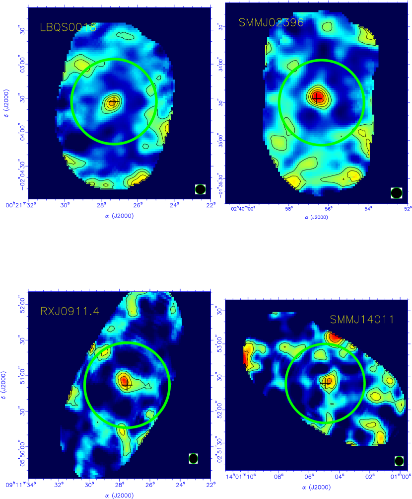
Figure 1.— Images of 350 µm emission for four galaxies with detections at $5\sigma$ or better. The black circle at the lower right show the size of beam. The colors of images from blue to red indicate increasing intensity for the pixels. The intensity contours start from the $2\sigma$ level, with a step of $2\sigma$. The $1\sigma$ levels for LBQS0018, SMMJ02396, RXJ0911.4 and SMMJ14011 are 5, 6, 21, 10 mJy within a 20″ aperture, respectively. The black cross in each panel marks the position of the CO peak. The green circles indicate the region within which detection is reliable. Emission towards the edge is not reliable because of decreased integration time and should be ignored.

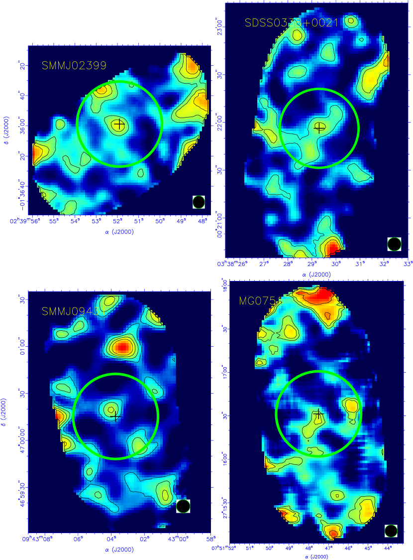
Figure 2.— Images of 350 µm emission for four galaxies with detections at less than $5\sigma$. The black circles at the lower right show the size of beam. The colors of images from blue to red indicate increasing intensity for the pixels. The intensity contours start from $1.5\sigma$, with a step of $1.5\sigma$, except for MG0751, in which the contour levels are $1.5\sigma$ and $2.2\sigma$. The $1\sigma$ levels for SMMJ02399, SDSS0038$+$0021, SMMJ09431 and MG0751 are 9, 9.5, 9, 16 mJy within a 20″ aperture, respectively. The black cross in each panel marks the position of the CO peak. The green circles indicate the region within which detection is reliable. Emission towards the edge is not reliable because of decreased integration time and should be ignored.

Figure 3.— The SEDs of all eight sources in the observed frame.

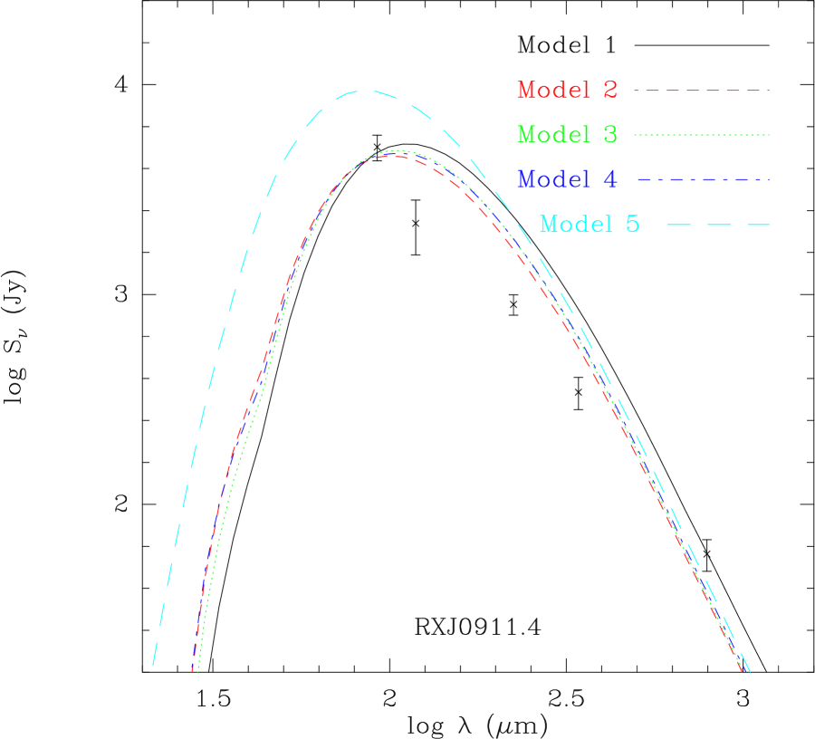
Figure 4.— The SED of the mean clump in RXJ0911.4 in the rest frame frequencies and flux densities at a distance of 10 kpc. The models are described in the text and in Table 4.

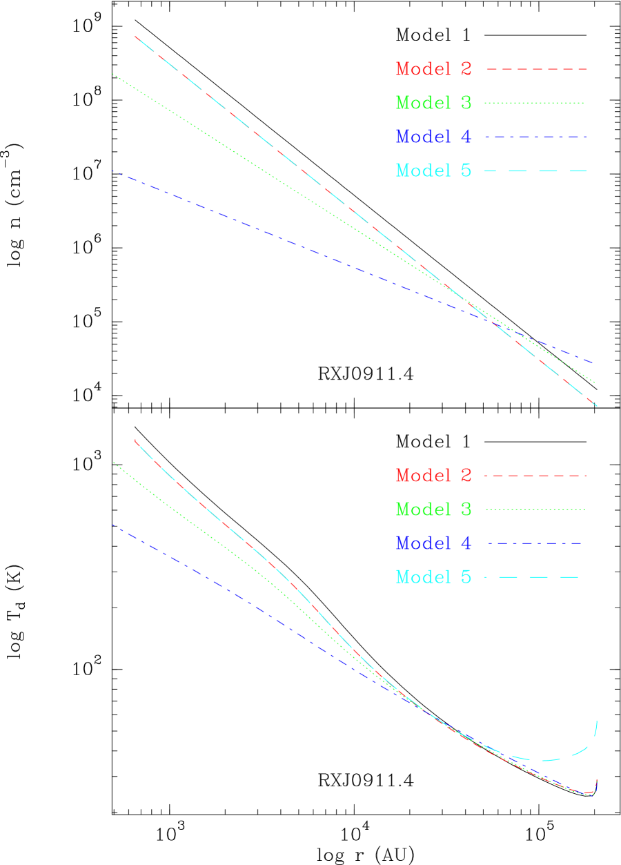
Figure 5.— The density and dust temperature are plotted versus radius for the models of the mean clump in RXJ0911.4. The models are described in the text and in Table 4.

Figure 6.— The SEDs for the standard clump, placed at 10 kpc, in six galaxies with detections are plotted as points with errorbars. The flux densities are shown at the rest wavelengths and the flux densities are scaled using equation 4. The solid lines are the best-fitting models from the radiative transfer modeling, as indicated in Table 4.

Figure 7.— (Top) The SED for the standard clump ($L=5\mbox{${}\times 10^{5}$}$ L_⊙), placed at 10 kpc, in SMM J02396. No model was able to fit the flux densities. (Bottom) The SED for a less luminous standard clump ($L=1\mbox{${}\times 10^{5}$}$ L_⊙), placed at 10 kpc, in SMM J02396. Now a model can provide a reasonable fit.

Figure 8.— (Top) The log of the luminosity to mass ratio from the radiative transport models is plotted versus the log of the dust temperature derived from the isothermal, optically thin fit. The solid line is the least squares fit to the data given by equation 6. The point at very low $T_{D}$ is SMM J02396, which has been excluded from the fit. (Bottom) The log of the optical depth at 100 µm from the best model is plotted versus the log of the dust temperature derived from the isothermal, optically thin fit. The solid line is the least squares fit to the data. The uncertainties assigned to the optical depth were 100%, to roughly indicate the dependence on model parameters. The point at very low $T_{D}$ is SMM J02396, which has been excluded from the fit.

References

- Andreani et al. (1999) Andreani, P., Franceschini, A., & Granato, G. 1999, MNRAS, 306, 16
- Bade et al. (1997) Bade, N., Siebert, J., Lopez, S., et al. 1997, A&A, 317, L13.
- Barvainis et al. (2002a) Barvainis, R., Alloin, D., & Bremer, M. 2002a, A&A, 385, 399.
- Barvainis & Ivison (2002b) Barvainis, R., & Ivison, R. 2002b, ApJ, 571, 712.
- Beelen et al. (2006) Beelen, A., Cox, P., Benford, D.J. et al. 2006, ApJ, 642, 694.
- Benford et al. (1999) Benford, D.J., Cox, P., Omont, A., et al. 1999, ApJ, 518, L65.
- Beuther et al. (2002) Beuther, H., Schilke, P., Menten, et al. 2002, ApJ, 566, 945.
- Blain et al. (2002) Blain, A. W., Smail, I., Ivison, R. J., Kneib, J.-P., & Frayer, D. T. 2002, Phys. Rep., 369, 111
- Carilli et al. (2001) Carilli, C. L., et al. 2001, ApJ, 555, 625.
- Chapman et al. (2004) Chapman, S. C., Smail, I., Blain, A. W., & Ivison, R. J. 2004, ApJ, 614, 671
- Combes et al. (1999) Combes, F., Maoli, R., & Omont, A. 1999, A&A, 345, 369
- Cowie et al. (2002) Cowie, L. L., Barger, A. J., & Kneib, J.-P. 2002, AJ, 123, 2197.
- Dickman et al. (1986) Dickman, R. L., Snell, R. L., & Schloerb, F. P. 1986, ApJ, 309, 326
- Dowell et al. (2003) Dowell, C.D., Allen, C.A., Babu, R. S., et al. 2003, Proc. SPIE, 4855, 73.
- Downes & Solomon (2003) Downes, D., & Solomon, P. M. 2003, ApJ, 582, 37.
- Draine (2003) Draine, B. T. 2003, ARA&A, 41, 241
- Efstathiou & Rowan-Robinson (2003) Efstathiou, A., & Rowan-Robinson, M. 2003, MNRAS, 343, 322
- Egan et al. (1988) Egan, M.P., Leung, C. M., & Spagna, G.F., Jr. 1988, Computer Physics Communications, 48, 271.
- Evans et al. (2001) Evans, N.J., II, Rawlings, J. M. C., Shirley, Y. L., et al. 2001, ApJ, 557, 193.
- Fan et al. (1999) Fan, X., et al. 1999, AJ, 118, 1.
- Foltz et al. (1989) Foltz, C.B., Chaffee, F.H., Hewett, P.C., et al. 1989, AJ, 98, 1959.
- Frayer et al. (1998) Frayer, D.T., Ivison, R.J., Scoville, N.Z., et al. 1998, ApJ, 506, L7.
- Frayer et al. (1999) Frayer, D.T., Ivison N.J., Scoville, N.Z. et al. 1999, ApJ, 514, L13.
- Gao and Solomon (2004a) Gao, Y., & Solomon, P.M. 2004a, ApJ, 606, 271.
- Gao and Solomon (2004b) Gao, Y., & Solomon, P.M. 2004b, ApJS, 152, 63.
- Genzel et al. (2003) Genzel, R., Baker, A. J., Tacconi, et al. 2003, ApJ, 584, 633.
- Granato et al. (1996) Granato, G. L., Danese, L., & Franceschini, A. 1996, ApJ, 460, L11
- Greve et al. (2005) Greve, T. R., et al. 2005, MNRAS, 359, 1165.
- Hainline et al. (2004) Hainline, L. J., Scoville, N. Z., Yun, M. S., Hawkins, D. W., Frayer, D. T., & Isaak, K. G. 2004, ApJ, 609, 61
- Ivison et al. (1998) Ivison, R. J., Smail, I., Le Borgne, et al. 1998, MNRAS, 298, 583.
- Ivison et al. (2000) Ivison, R.J., Smail, I., Barger, et al. 2000, MNRAS, 315, 209.
- Izaak (2004) Izaak, K.G. 2004, private communication.
- Kennicutt (1998) Kennicutt, R. C., Jr. 1998, ARA&A, 36, 189.
- Kneib et al. (2000) Kneib, J.-P., Cohen, J. G., & Hjorth, J. 2000, ApJ, 544, L35.
- Kovács (2006a) Kovács, A. 2006, arXiv:0805.3928v2.
- Kovács (2006b) Kovács, A. 2006b, PhD thesis, Caltech.
- Kovács et al. (2006c) Kovács, A., Chapman, S. C., Dowell, et al. 2006c, ApJ, 650, 592.
- Leong (2005) Leong,M.M. 2005, URSI Conf. Sec., J3-J10,426
- Maiolino et al. (2007) Maiolino, R., et al. 2007, A&A, 472, L33.
- Mueller et al. (2002) Mueller, K.E., Shirley, Y.L., Evans, N.J., II, et al. 2002, ApJS, 143, 469.
- Narayanan et al. (2009a) Narayanan, D., Hayward, C. C., Cox, T. J., Hernquist, L., Jonsson, P., Younger, J. D., & Groves, B. 2009, arXiv:0904.0004
- Narayanan et al. (2009b) Narayanan, D., Cox, T. J., Hayward, C., Younger, J. D., & Hernquist, L. 2009, arXiv:0905.2184
- Neri et al. (2003) Neri, R., et al. 2003, ApJ, 597, L113.
- Ossenkopf and Henning (1994) Ossenkopf, V. & Henning, T. 1994, A&A, 291, 943.
- Priddey et al. (2003a) Priddey, R.S., Isaak, K.G., McMahon, R. G., et al. 2003a, MNRAS, 339, 1183.
- Priddey et al. (2003b) Priddey, R. S., Isaak, K. G., McMahon, et al. 2003, MNRAS, 344, L74.
- Rowan-Robinson (2000) Rowan-Robinson, M. 2000, MNRAS, 316, 885
- Sanders and Mirabel (1996) Sanders, D.B., & Mirabel, I.F. 1996, ARA&A, 34, 749.
- Smail et al. (2002) Smail, I., Ivison, R.J., Blain, A. W., et al. 2002, MNRAS, 331, 495.
- Solomon & Vanden Bout (2005) Solomon, P.M. & Vanden Bout, P.A. 2005, ARA&A, 43, 677.
- Solomon et al. (1987) Solomon, P. M., Rivolo, A. R., Barrett, J., & Yahil, A. 1987, ApJ, 319, 730
- Soucail et al. (1999) Soucail, G., Kneib, J.P., Bezecourt, J., et al. 1999, A&A, 343, L70.
- Spergel et al. (2007) Spergel, D.N., et al. 2007, ApJS, 170, 377.
- van der Tak et al. (1999) van der Tak, F. F. S., van Dishoeck, E. F., Evans, N. J., II, et al. 1999, ApJ, 522, 991.
- Wang et al. (2008a) Wang, R., Carilli, C.L., Wagg, J., et al. 2008a, AJ, 135, 1201.
- Wang et al. (2008b) Wang, R., Carilli, C.L., Wagg, J., et al. 2008b, ApJ, 687, 848.
- Weiß et al. (2003) Weiß, A., Henkel, C., Downes, D., et al. 2003, A&A, 409, L41.
- Weiß et al. (2005) Weiß, A., Downes, D., Henkel, C., et al. 2005, A&A, 429, L25.
- Weiß et al. (2007) Weiß, A., Downes, D., Neri, R., Walter, F., Henkel, C., Wilner, D. J., Wagg, J., & Wiklind, T. 2007, A&A,
- Wu et al. (2005) Wu, J., Evans, N.J. II, Gao, Y., et al. 2005, ApJ, 635, L173.
- Wu et al. (2007) Wu, J, Dunham, M. M.; Evans, N. J., II, Bourke, T. L., Young, C. H., 2007, AJ, 133, 1560
- Wu et al. (2009) Wu, J., Evans, N. J., II, Shirley, Y. L., & Knez, C., in prep.