Cosmological perturbation theory for baryons and dark matter I:
one-loop corrections in the RPT framework

Gábor Somogyi Gabor.Somogyi@desy.de Deutsches Elektronensynchrotron DESY, Platanenallee 6, D-15738 Zeuthen, Germany Institute for Theoretical Physics, University of Zurich, CH-8037 Zurich, Switzerland    Robert E. Smith res@physik.unizh.ch Institute for Theoretical Physics, University of Zurich, CH-8037 Zurich, Switzerland
Abstract

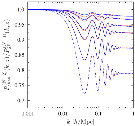
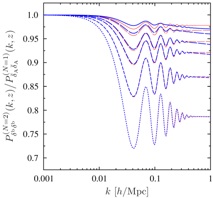
We generalize the “renormalized” perturbation theory (RPT) formalism of Crocce and Scoccimarro (2006a) to deal with multiple fluids in the Universe and here we present the complete calculations up to the one-loop level in the RPT. We apply this approach to the problem of following the non-linear evolution of baryon and cold dark matter (CDM) perturbations, evolving from the distinct sets of initial conditions, from the high redshift post-recombination Universe right through to the present day. In current theoretical and numerical models of structure formation, it is standard practice to treat baryons and CDM as an effective single matter fluid – the so called dark matter only modeling. In this approximation, one uses a weighed sum of late time baryon and CDM transfer functions to set initial mass fluctuations. In this paper we explore whether this approach can be employed for high precision modeling of structure formation. We show that, even if we only follow the linear evolution, there is a large-scale scale-dependent bias between baryons and CDM for the currently favored WMAP5 ΛΛ\LambdaCDM model. This time evolving bias is significant (>1%)absentpercent1(>1\%) until the present day, when it is driven towards unity through gravitational relaxation processes. Using the RPT formalism we test this approximation in the non-linear regime. We show that the non-linear CDM power spectrum in the 2-component fluid differs from that obtained from an effective mean-mass 1-component fluid by 3%similar-toabsentpercent3\sim 3\% on scales of order k0.05hMpc1similar-to𝑘0.05superscriptMpc1k\sim 0.05\,h\,{\rm Mpc}^{-1} at z=10𝑧10z=10, and by 0.5%similar-toabsentpercent0.5\sim 0.5\% at z=0𝑧0z=0. However, for the case of the non-linear evolution of the baryons the situation is worse and we find that the power spectrum is suppressed, relative to the total matter, by 15%similar-toabsentpercent15\sim 15\% on scales k0.05hMpc1similar-to𝑘0.05superscriptMpc1k\sim 0.05\,h\,{\rm Mpc}^{-1} at z=10𝑧10z=10, and by 35%similar-toabsent3percent5\sim 3-5\% at z=0𝑧0z=0. Importantly, besides the suppression of the spectrum, the Baryonic Acoustic Oscillation (BAO) features are amplified for baryon and slightly damped for CDM spectra. If we compare the total matter power spectra in the 2- and 1-component fluid approaches, then we find excellent agreement, with deviations being <0.5%absentpercent0.5<0.5\% throughout the evolution. Consequences: high precision modeling of the large-scale distribution of baryons in the Universe can not be achieved through an effective mean-mass 1-component fluid approximation; detection significance of BAO will be amplified in probes that study baryonic matter, relative to probes that study the CDM or total mass only. The CDM distribution can be modeled accurately at late times and the total matter at all times. This is good news for probes that are sensitive to the total mass, such as gravitational weak lensing as existing modeling techniques are good enough. Lastly, we identify an analytic approximation that greatly simplifies the evaluation of the full PT expressions, and it is better than <1%absentpercent1<1\% over the full range of scales and times considered.

I Introduction

In the current paradigm for structure formation in the Universe, it is supposed that there was an initial period of inflation, during which, quantum fluctuations were generated and inflated up to super-horizon scales; producing a near scale-invariant and near Gaussian set of primordial potential fluctuations. At the end of inflation the Universe is reheated, and particles and radiation are synthesized. In this hot early phase, cold thermal relics are also produced, these particles interact gravitationally and possibly through the weak interaction – dubbed Cold Dark Matter (CDM). Prior to recombination photons are coupled to electrons through Thompson scattering, and in turn electrons to baryonic nuclei through the Coulomb interaction. Baryon fluctuations are pressure supported on scales smaller than the sound horizon scale. Subsequent to recombination photons free-stream out of perturbations and baryons cool into the CDM potential wells. Structure formation then proceeds in a hierarchical way with small objects collapsing first and then merging to form larger objects. Eventually, sufficiently dense gas wells are accumulated and galaxies form. At late times the Universe switches from a decelerating phase of expansion to an accelerated phase. This is attributed to the non-zero constant energy-density of the vacuum. This paradigm has been dubbed: ΛΛ\LambdaCDM (Peebles and Ratra, 2003; Spergel et al., 2007; Komatsu et al., 2009).

The present day energy-density budget for the ΛΛ\LambdaCDM model is distributed into several components, which in units of the critical density are: vacuum energy ΩΛ,00.73subscriptΩΛ00.73\Omega_{\Lambda,0}\approx 0.73, matter Ωm,00.27subscriptΩm00.27\Omega_{\mathrm{m},0}\approx 0.27, neutrinos Ων,0102less-than-or-similar-tosubscriptΩ𝜈0superscript102\Omega_{\nu,0}\lesssim 10^{-2} and radiation Ωr,05×104subscriptΩr05superscript104\Omega_{\mathrm{r},0}\approx 5\times 10^{-4}. The matter distribution can be subdivided further into contributions from CDM and baryons, with present day values Ωc0.225subscriptΩc0.225\Omega_{\mathrm{c}}\approx 0.225 and Ωb0.045subscriptΩb0.045\Omega_{\mathrm{b}}\approx 0.045. The detailed physics for the evolution of the radiation, CDM, baryon and neutrino fluctuations (δr,δc,δb,δνsuperscript𝛿rsuperscript𝛿csuperscript𝛿bsuperscript𝛿𝜈\delta^{\mathrm{r}},\delta^{\mathrm{c}},\delta^{\mathrm{b}},\delta^{\nu}), from the early Universe through to recombination can be obtained by solving the Einstein–Boltzmann equations. These are a set of coupled non-linear partial differential equations, however while the fluctuations are small they may be linearized and solved (for a review see Ma and Bertschinger, 1995; Seljak and Zaldarriaga, 1996). At later times these fluctuations enter a phase of non-linear growth. Their evolution during this period can no longer be described accurately using the linear Einstein–Boltzmann theory and must be followed using higher order perturbation theory (hereafter PT) techniques Bernardeau et al. (2002) or more directly through N𝑁N-body simulations Bertschinger (2001).

Refer to caption
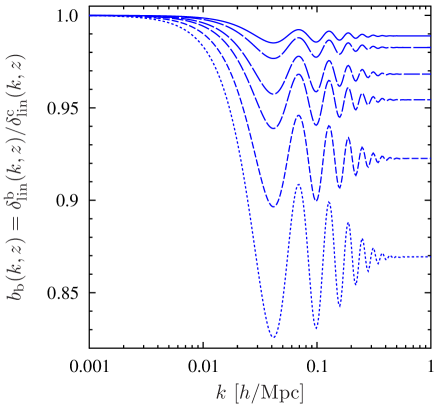
Figure 1: Baryon bias as a function of inverse spatial scale, where we have defined the baryon bias bb(k,z)δlinb(k,z)/δlinc(k,z)subscript𝑏b𝑘𝑧subscriptsuperscript𝛿blin𝑘𝑧subscriptsuperscript𝛿clin𝑘𝑧b_{\mathrm{b}}(k,z)\equiv\delta^{\mathrm{b}}_{\mathrm{lin}}(k,z)/\delta^{\mathrm{c}}_{\mathrm{lin}}(k,z), and used Eqs (79) and (80) from §II.6. Solid through to dashed lines show results for redshifts z={0,1.0,3.0,5.0,10.0,20.0}𝑧01.03.05.010.020.0z=\{0,1.0,3.0,5.0,10.0,20.0\}.

The cross-over from the linear to the non-linear theory is, in general, not straightforward. Most of the theoretical and numerical approaches to this latter task were developed during the previous two decades, during which time the Standard CDM model was favored: essentially Einstein-de Sitter spacetime, Ωm=1subscriptΩm1\Omega_{\mathrm{m}}=1, with energy-density dominated by CDM 97%greater-than-or-equivalent-toabsentpercent97\gtrsim 97\%, and baryons contributing 3%less-than-or-similar-toabsentpercent3\lesssim 3\% to the total matter. For this case it is natural to assume that the CDM fluctuations dominate the gravitational potentials at nearly all times, with baryons playing little role in the formation of large-scale structure (see for example Efstathiou et al., 1985; Thomas and Couchman, 1992; Couchman et al., 1995). Thus, one simply requires a transfer function for the CDM distribution at some late time, to model the evolution of both components.

In the latter part of the 1990s, cosmological tests pointed towards the ΛΛ\LambdaCDM paradigm, and it was recognized that baryons should play some role in shaping the transfer function of matter fluctuations (Ma and Bertschinger, 1995; Sugiyama, 1995; Eisenstein and Hu, 1998; Meiksin et al., 1999). However, rather than attempting to follow the CDM and baryons as separate fluids evolving from distinct sets of initial conditions, a simpler approximate scheme was adopted. This scheme is currently standard practice for all studies of structure formation in the Universe (Pearce et al., 2001; Teyssier, 2002; Springel, 2005, 2009). It can be summarized as follows:

  1. 1.

    Fix the cosmological model, specifying ΩcsubscriptΩc\Omega_{\mathrm{c}} and ΩbsubscriptΩb\Omega_{\mathrm{b}}, and hence the fraction of baryons, fbsuperscript𝑓bf^{\rm b}. Solve for the evolution of all perturbed species using the linearized coupled Einstein–Boltzmann equations. Obtain transfer functions at z=0𝑧0z=0, where CDM and baryons are fully relaxed: i.e. Tc(k,z=0)Tb(k,z=0)superscript𝑇c𝑘𝑧0superscript𝑇b𝑘𝑧0T^{\mathrm{c}}(k,z=0)\approx T^{\mathrm{b}}(k,z=0), where Tcsuperscript𝑇cT^{\mathrm{c}} and Tbsuperscript𝑇bT^{\mathrm{b}} are the transfer functions of the CDM and baryons, respectively.

  2. 2.

    Use the transfer functions to generate the linear matter power spectrum, normalized to the present day: i.e. Pδ¯δ¯(𝐤,z=0)[(1fb)Tc(k,z=0)+fbTb(k,z=0)]2Akn[Tc(k,z=0)]2Akn,subscript𝑃¯𝛿¯𝛿𝐤𝑧0superscriptdelimited-[]1superscript𝑓bsuperscript𝑇c𝑘𝑧0superscript𝑓bsuperscript𝑇b𝑘𝑧02𝐴superscript𝑘𝑛superscriptdelimited-[]superscript𝑇c𝑘𝑧02𝐴superscript𝑘𝑛P_{\bar{\delta}\bar{\delta}}({\bf k},z=0)\approx\left[(1-f^{\rm b})T^{\mathrm{c}}(k,z=0)+f^{\rm b}T^{\mathrm{b}}(k,z=0)\right]^{2}Ak^{n}\approx[T^{\mathrm{c}}(k,z=0)]^{2}Ak^{n}\ , where the total matter fluctuation is δ¯=(1fb)δc+fbδb¯𝛿1superscript𝑓bsuperscript𝛿csuperscript𝑓bsuperscript𝛿b\bar{\delta}=(1-f^{\rm b})\delta^{\mathrm{c}}+f^{\rm b}\delta^{\mathrm{b}}.

  3. 3.

    Scale this power spectrum back to the initial time zisubscript𝑧𝑖z_{i}, using the linear growth factor for the total matter fluctuation δ¯¯𝛿\bar{\delta}, which obtains from solving the equations of motion for a single fluid.

  4. 4.

    Generate the initial CDM density field and assume that the baryons are perfect tracers of the CDM.

  5. 5.

    Evolve this effective CDM+baryon fluid under gravity using full non-linear equations of motion, either as a single fluid for dark matter only, or as a 2-component fluid if hydrodynamics are also to be followed.

This effective description for the formation of structure becomes poor as the baryon fraction fb=Ωb/Ωmsuperscript𝑓bsubscriptΩbsubscriptΩmf^{\rm b}=\Omega_{\mathrm{b}}/\Omega_{\mathrm{m}} approaches O(1)similar-toabsent𝑂1\sim O(1), and for the currently favored WMAP5 cosmology fb0.17superscript𝑓b0.17f^{\rm b}\approx 0.17. In fact, in linear theory the gravitational relaxation between baryonic and dark matter components is only achieved at the level of <1%absentpercent1<1\% by z=0𝑧0z=0. Moreover, as can be seen in Fig. 1 there is a non-trivial scale-dependent bias between baryons and dark matter that exists right through to the present day 111Note that we have defined the baryon bias bb(k,z)δlinb(k,z)/δlinc(k,z)subscript𝑏b𝑘𝑧subscriptsuperscript𝛿blin𝑘𝑧subscriptsuperscript𝛿clin𝑘𝑧b_{\mathrm{b}}(k,z)\equiv\delta^{\mathrm{b}}_{\mathrm{lin}}(k,z)/\delta^{\mathrm{c}}_{\mathrm{lin}}(k,z), where these linear fluctuations are given by Eqs (79) and (80) from §II.6. In this analysis we have neglected any residual effect of the coupling between the photons and the baryons, and have assumed that the baryons are cold at z=100𝑧100z=100, hence pbρT0proportional-tosubscript𝑝b𝜌𝑇similar-to0p_{\rm b}\propto\rho T\sim 0. Furthermore, this result is sensitive to our choice for the initial δisubscript𝛿𝑖\delta_{i} and θisubscript𝜃𝑖\theta_{i}, and indeed had we chosen the initial baryon and CDM velocity fields to be proportional to the total matter fluctuation, then these effects would be slightly reduced. However, the resultant bias will still remain non-negligible.. Failing, to take these biases into account may lead to non-negligible systematic errors in studies that attempt to obtain cosmological constraints from Large-Scale Structure (LSS) tests. With the next generation of LSS tests aiming to achieving 1% precision in measurements of the matter power spectrum Albrecht et al. (2006); Peacock et al. (2006), it seems timely to investigate whether such modeling assumptions may impact inferences. Where we expect such systematic effects to play an important role is for studies based on baryonic physics such as: using 21cm emission from neutral hydrogen to trace mass density at the epoch of reionization zreion10subscript𝑧reion10z_{\rm reion}\approx 10 (Zhang et al., 2004; Iliev et al., 2006; Furlanetto et al., 2006; Pillepich et al., 2007); and studies of the Lyman alpha forest to probe the matter power spectrum (Croft et al., 1998; McDonald et al., 2006).

In this, the first in a series of papers, we test whether this effective procedure can indeed be employed to follow, at high precision, the non-linear growth of structure formation in baryon and CDM fluids, from recombination right through to the present day. We do this by generalizing the matrix based “renormalized” perturbation theory (RPT) 222It appears to us that what may be implemented in the RPT framework is not so much what would usually be understood as the “perturbative renormalization” of the theory, but rather a “resummation” of the perturbative series, in some specific approximation (the “high-k𝑘k” limit). We will continue to use the acronym RPT to refer to the method, but would suggest that it is more properly read as resummed, and not renormalized perturbation theory. techniques of Crocce and Scoccimarro (2006a, b, 2008) to an arbitrary number of gravitating fluids. In this paper we content our selves with calculating the observables up to the one-loop level in the theory. In a future paper we consider the resummation to arbitrary orders (Somogyi & Smith 2009, in preparation).

The late-time linear theory evolution of coupled baryon and CDM fluctuations, with sudden late time reionization of the inter-galactic medium was studied by (Nusser, 2000; Matarrese and Mohayaee, 2002). Recently, (Shoji and Komatsu, 2009) explored a similar system using non-linear PT techniques. The work presented by these authors differs from that presented here in a number of fundamental ways. Firstly, these authors have assumed that, on large scales, baryons and CDM fluctuations evolve with the same initial conditions and that the only physical difference between the two fluids arises on small scales, where galaxy formation processes are able to provide some pressure support. They model this with a fixed comoving-scale Jeans criterion. In this work we are not so much interested in following how small-scale baryonic collapse feeds back on the mass distribution, but are more interested in following the very large-scale baryon and CDM fluctuations, initialized with their correct post-recombination spatial distributions, into the non-linear regime. Secondly, their work was developed within standard PT, the problems associated with this formalism are well documented (Bernardeau et al., 2002). Here, we develop the more successful RPT approach (Crocce and Scoccimarro, 2006a). In passing, we note that a number of additional complimentary approaches and extensions to single-fluid RPT have recently been developed (Matarrese and Pietroni, 2007, 2008; Bernardeau et al., 2008; Pietroni, 2008; Matsubara, 2008). In addition, there has recently been progress on realistic modeling of massive neutrinos and CDM (Wong, 2008; Saito et al., 2008; Ichiki et al., 2009; Brandbyge et al., 2008; Brandbyge and Hannestad, 2009a, b; Lesgourgues et al., 2009), for simplicity we shall assume that neutrinos play a negligible role.

The paper is broken down as follows: In §II we set up the theoretical formalism: presenting the coupled equations of motion for the N𝑁N-component fluid. Then we show how, when written in matrix form, the equations may be solved at linear order. We discuss generalized initial conditions, and then discuss the specific case of baryons and CDM. In §III we develop the non-linear PT expansion for the solutions, and show that they may be constructed to arbitrary order using a set of Feynman rules. In §IV we discuss the two-point statistics of the fields, which we take as our lowest order observables. In §V we give specific details of how we calculate the one-loop corrections in our theory. In §VI we present results for various quantities of interest. In §VII we give details of an approximate RPT scheme, which matches the exact calculation to within <1%absentpercent1<1\%, for all times of interest and on all scales where the perturbation theory is valid. Finally, in §VIII we draw our conclusions.

II Equations of motion

II.1 Standard form

For an N𝑁N-component fluid in a uniformly expanding spacetime, the relevant equations of motion are, conservation of mass, momentum, and the Poisson equation. These may be written (i=1,,N𝑖1𝑁i=1,\ldots,N labels the i𝑖i-th component) (Bernardeau et al., 2002):

δi(x,τ)τ+[(1+δi(x,τ))vi(x,τ)]=0;subscript𝛿𝑖x𝜏𝜏delimited-[]1subscript𝛿𝑖x𝜏subscriptv𝑖x𝜏0\displaystyle\frac{\partial\delta_{i}(\hbox{\bf x},\tau)}{\partial\tau}+\nabla\cdot[(1+\delta_{i}(\hbox{\bf x},\tau))\hbox{\bf v}_{i}(\hbox{\bf x},\tau)]=0\,; (1)
vi(x,τ)τ+(τ)vi(x,τ)+(vi(x,τ))vi(x,τ)=Φ(x,τ);subscriptv𝑖x𝜏𝜏𝜏subscriptv𝑖x𝜏subscriptv𝑖x𝜏subscriptv𝑖x𝜏Φx𝜏\displaystyle\frac{\partial\hbox{\bf v}_{i}(\hbox{\bf x},\tau)}{\partial\tau}+{\cal H}(\tau)\hbox{\bf v}_{i}(\hbox{\bf x},\tau)+(\hbox{\bf v}_{i}(\hbox{\bf x},\tau)\cdot\nabla)\hbox{\bf v}_{i}(\hbox{\bf x},\tau)=-\nabla\Phi(\hbox{\bf x},\tau)\,; (2)
2Φ(x,τ)=4πGa2i=1Nρ¯i(τ)δi(x,τ)=32Ωm(τ)2(τ)i=1Nwiδi(x,τ).superscript2Φx𝜏4𝜋𝐺superscript𝑎2superscriptsubscript𝑖1𝑁subscript¯𝜌𝑖𝜏subscript𝛿𝑖x𝜏32subscriptΩm𝜏superscript2𝜏superscriptsubscript𝑖1𝑁subscript𝑤𝑖subscript𝛿𝑖x𝜏\displaystyle\nabla^{2}\Phi(\hbox{\bf x},\tau)=4\pi Ga^{2}\sum_{i=1}^{N}\bar{\rho}_{i}(\tau)\delta_{i}(\hbox{\bf x},\tau)=\frac{3}{2}\Omega_{\mathrm{m}}(\tau){\cal H}^{2}(\tau)\sum_{i=1}^{N}w_{i}\delta_{i}(\hbox{\bf x},\tau)\,. (3)

where τ𝜏\tau is conformal time dτdt/ad𝜏d𝑡𝑎{\mathrm{d}}\tau\equiv{\mathrm{d}}t/a, with a𝑎a the scale factor. Here we have introduced the density perturbations in each component as δi(x,τ)ρi(x,τ)/ρ¯i1=ρi(x,τ)/wiρ¯m1subscript𝛿𝑖x𝜏subscript𝜌𝑖x𝜏subscript¯𝜌𝑖1subscript𝜌𝑖x𝜏subscript𝑤𝑖subscript¯𝜌m1\delta_{i}(\hbox{\bf x},\tau)\equiv\rho_{i}(\hbox{\bf x},\tau)/\bar{\rho}_{i}-1=\rho_{i}(\hbox{\bf x},\tau)/w_{i}\bar{\rho}_{\rm m}-1, where ρisubscript𝜌𝑖\rho_{i} and ρ¯isubscript¯𝜌𝑖\bar{\rho}_{i} are the density and mean density. vi(x,τ)subscriptv𝑖x𝜏\hbox{\bf v}_{i}(\hbox{\bf x},\tau) is the peculiar velocity. (τ)=dlna/dτ𝜏d𝑎d𝜏{\cal H}(\tau)={\mathrm{d}}\ln a/{\mathrm{d}}\tau is the conformal Hubble parameter, related to the usual Hubble parameter, Ha˙/a𝐻˙𝑎𝑎H\equiv\dot{a}/a, through (τ)=aH𝜏𝑎𝐻{\cal H}(\tau)=aH. The wiΩi/Ωmsubscript𝑤𝑖subscriptΩ𝑖subscriptΩmw_{i}\equiv\Omega_{i}/\Omega_{\mathrm{m}} are the fractional contributions of each fluid species to the total matter density. They are constant in time, and normalized

i=1Nwi=1.superscriptsubscript𝑖1𝑁subscript𝑤𝑖1\sum_{i=1}^{N}w_{i}=1\,. (4)

In the above we have also expressed the mean energy-density in each species in units of the critical density,

Ωi(τ)ρ¯i(τ)ρcrit(τ)=8πGρ¯i(τ)3a22(τ),subscriptΩ𝑖𝜏subscript¯𝜌𝑖𝜏subscript𝜌crit𝜏8𝜋𝐺subscript¯𝜌𝑖𝜏3superscript𝑎2superscript2𝜏\Omega_{i}(\tau)\equiv\frac{\bar{\rho}_{i}(\tau)}{\rho_{\rm crit}(\tau)}=\frac{8\pi G\bar{\rho}_{i}(\tau)}{3a^{2}{\cal H}^{2}(\tau)}\ , (5)

and with subscript 0 denoting present day quantities, Ωi,0=Ωi(τ=τ0)subscriptΩ𝑖0subscriptΩ𝑖𝜏subscript𝜏0\Omega_{i,0}=\Omega_{i}(\tau=\tau_{0}). Finally, the Hubble and density parameters of each species are related through the Friedmann equation, which can be written:

2(τ)=a202[Ωm,0a3+ΩΛ,0+ΩK,0a2];ΩK,01Ωm,0ΩΛ,0.formulae-sequencesuperscript2𝜏superscript𝑎2superscriptsubscript02delimited-[]subscriptΩm0superscript𝑎3subscriptΩΛ0subscriptΩ𝐾0superscript𝑎2subscriptΩ𝐾01subscriptΩm0subscriptΩΛ0{\cal H}^{2}(\tau)=a^{-2}{\cal H}_{0}^{2}\left[\Omega_{\mathrm{m},0}a^{-3}+\Omega_{\Lambda,0}+\Omega_{K,0}a^{-2}\right]\ ;\ \ \ \ \Omega_{K,0}\equiv 1-\Omega_{\mathrm{m},0}-\Omega_{\Lambda,0}\ . (6)

Taking the divergence of Eq. (2) and using Eq. (3) to eliminate ΦΦ\Phi, we obtain

Θi(x,τ)τ+(τ)Θi(x,τ)+j,k[j(vi)k(x,τ)][k(vi)j(x,τ)]+(vi(x,τ))Θi(x,τ)subscriptΘ𝑖x𝜏𝜏𝜏subscriptΘ𝑖x𝜏subscript𝑗𝑘delimited-[]subscript𝑗subscriptsubscriptv𝑖𝑘x𝜏delimited-[]subscript𝑘subscriptsubscriptv𝑖𝑗x𝜏subscriptv𝑖x𝜏subscriptΘ𝑖x𝜏\displaystyle\frac{\partial\Theta_{i}(\hbox{\bf x},\tau)}{\partial\tau}+{\cal H}(\tau)\Theta_{i}(\hbox{\bf x},\tau)+\sum_{j,k}[\partial_{j}(\hbox{\bf v}_{i})_{k}(\hbox{\bf x},\tau)][\partial_{k}(\hbox{\bf v}_{i})_{j}(\hbox{\bf x},\tau)]+(\hbox{\bf v}_{i}(\hbox{\bf x},\tau)\cdot\nabla)\Theta_{i}(\hbox{\bf x},\tau)
=32Ωm(τ)2(τ)j=1Nwjδj(x,τ),absent32subscriptΩm𝜏superscript2𝜏superscriptsubscript𝑗1𝑁subscript𝑤𝑗subscript𝛿𝑗x𝜏\displaystyle\qquad\qquad=-\frac{3}{2}\Omega_{\mathrm{m}}(\tau){\cal H}^{2}(\tau)\sum_{j=1}^{N}w_{j}\delta_{j}(\hbox{\bf x},\tau)\,, (7)

where we have set v(x,τ)=Θ(x,τ)vx𝜏Θx𝜏\nabla\cdot\hbox{\bf v}(\hbox{\bf x},\tau)=\Theta(\hbox{\bf x},\tau) and j𝑗j and k𝑘k denote vector components. Next, we go to Fourier space. For a quantity A(x,τ)𝐴x𝜏A(\hbox{\bf x},\tau), we define the Fourier transform, A~(k,τ)~𝐴k𝜏\tilde{A}(\hbox{\bf k},\tau) and its inverse, as follows

A(x,τ)=d3keikxA~(k,τ)A~(k,τ)=d3x(2π)3eikxA(x,τ).formulae-sequence𝐴x𝜏superscriptd3ksuperscripteikx~𝐴k𝜏~𝐴k𝜏superscriptd3xsuperscript2𝜋3superscripteikx𝐴x𝜏A(\hbox{\bf x},\tau)=\int{\mathrm{d}}^{3}\hbox{\bf k}\,{\mathrm{e}}^{{\mathrm{i}}\hbox{\bf k}\cdot\hbox{\bf x}}\tilde{A}(\hbox{\bf k},\tau)\quad\Leftrightarrow\quad\tilde{A}(\hbox{\bf k},\tau)=\int\frac{{\mathrm{d}}^{3}\hbox{\bf x}}{(2\pi)^{3}}{\mathrm{e}}^{-{\mathrm{i}}\hbox{\bf k}\cdot\hbox{\bf x}}A(\hbox{\bf x},\tau)\ . (8)

Assuming vi(x,τ)subscriptv𝑖x𝜏\hbox{\bf v}_{i}(\hbox{\bf x},\tau) to be irrotational, there exists a scalar field ui(x,τ)subscript𝑢𝑖x𝜏u_{i}(\hbox{\bf x},\tau), such that vi(x,τ)=ui(x,τ)subscriptv𝑖x𝜏subscript𝑢𝑖x𝜏\hbox{\bf v}_{i}(\hbox{\bf x},\tau)=-\nabla u_{i}(\hbox{\bf x},\tau) and thus

v~i(k,τ)=iku~i(k,τ),Θ~i(k,τ)=k2u~i(k,τ)v~i(k,τ)=ikΘ~i(k,τ)k2.formulae-sequencesubscript~v𝑖k𝜏iksubscript~𝑢𝑖k𝜏formulae-sequencesubscript~Θ𝑖k𝜏superscriptk2subscript~𝑢𝑖k𝜏subscript~v𝑖k𝜏iksubscript~Θ𝑖k𝜏superscriptk2\tilde{\hbox{\bf v}}_{i}(\hbox{\bf k},\tau)=-{\mathrm{i}}\hbox{\bf k}\tilde{u}_{i}(\hbox{\bf k},\tau)\,,\quad\tilde{\Theta}_{i}(\hbox{\bf k},\tau)=\hbox{\bf k}^{2}\tilde{u}_{i}(\hbox{\bf k},\tau)\quad\Rightarrow\quad\tilde{\hbox{\bf v}}_{i}(\hbox{\bf k},\tau)=-{\mathrm{i}}\hbox{\bf k}\frac{\tilde{\Theta}_{i}(\hbox{\bf k},\tau)}{\hbox{\bf k}^{2}}\,. (9)

On inserting this relation into the equations of motion we find:

δ~i(k,τ)τ+Θ~i(k,τ)+d3k1d3k2δD(kk1k2)(1+k1k2k22)δ~i(k1,τ)Θ~i(k2,τ)=0;subscript~𝛿𝑖k𝜏𝜏subscript~Θ𝑖k𝜏superscriptd3subscriptk1superscriptd3subscriptk2superscript𝛿𝐷ksubscriptk1subscriptk21subscriptk1subscriptk2superscriptsubscriptk22subscript~𝛿𝑖subscriptk1𝜏subscript~Θ𝑖subscriptk2𝜏0\displaystyle\frac{\partial\tilde{\delta}_{i}(\hbox{\bf k},\tau)}{\partial\tau}+\tilde{\Theta}_{i}(\hbox{\bf k},\tau)+\int{\mathrm{d}}^{3}\hbox{\bf k}_{1}\,{\mathrm{d}}^{3}\hbox{\bf k}_{2}\,\delta^{D}(\hbox{\bf k}-\hbox{\bf k}_{1}-\hbox{\bf k}_{2})\left(1+\frac{\hbox{\bf k}_{1}\cdot\hbox{\bf k}_{2}}{\hbox{\bf k}_{2}^{2}}\right)\tilde{\delta}_{i}(\hbox{\bf k}_{1},\tau)\tilde{\Theta}_{i}(\hbox{\bf k}_{2},\tau)=0\,; (10)
Θ~i(k,τ)τ+(τ)Θ~i(k,τ)+32Ωm(τ)2(τ)j=1Nwjδ~j(k,τ)subscript~Θ𝑖k𝜏𝜏𝜏subscript~Θ𝑖k𝜏32subscriptΩm𝜏superscript2𝜏superscriptsubscript𝑗1𝑁subscript𝑤𝑗subscript~𝛿𝑗k𝜏\displaystyle\frac{\partial\tilde{\Theta}_{i}(\hbox{\bf k},\tau)}{\partial\tau}+{\cal H}(\tau)\tilde{\Theta}_{i}(\hbox{\bf k},\tau)+\frac{3}{2}\Omega_{\mathrm{m}}(\tau){\cal H}^{2}(\tau)\sum_{j=1}^{N}w_{j}\tilde{\delta}_{j}(\hbox{\bf k},\tau)
+d3k1d3k2δD(kk1k2)[(k1+k2)2k1k22k12k22]Θ~i(k1,τ)Θ~i(k2,τ)=0.superscriptd3subscriptk1superscriptd3subscriptk2superscript𝛿𝐷ksubscriptk1subscriptk2delimited-[]superscriptsubscriptk1subscriptk22subscriptk1subscriptk22superscriptsubscriptk12superscriptsubscriptk22subscript~Θ𝑖subscriptk1𝜏subscript~Θ𝑖subscriptk2𝜏0\displaystyle\qquad\qquad\qquad+\int{\mathrm{d}}^{3}\hbox{\bf k}_{1}\,{\mathrm{d}}^{3}\hbox{\bf k}_{2}\,\delta^{D}(\hbox{\bf k}-\hbox{\bf k}_{1}-\hbox{\bf k}_{2})\left[\frac{(\hbox{\bf k}_{1}+\hbox{\bf k}_{2})^{2}\hbox{\bf k}_{1}\cdot\hbox{\bf k}_{2}}{2\hbox{\bf k}_{1}^{2}\hbox{\bf k}_{2}^{2}}\right]\tilde{\Theta}_{i}(\hbox{\bf k}_{1},\tau)\tilde{\Theta}_{i}(\hbox{\bf k}_{2},\tau)=0\,. (11)

Finally, we introduce the variable θ~i(k,τ)Θ~i(k,τ)/(τ)subscript~𝜃𝑖k𝜏subscript~Θ𝑖k𝜏𝜏\tilde{\theta}_{i}(\hbox{\bf k},\tau)\equiv-\tilde{\Theta}_{i}(\hbox{\bf k},\tau)/{\cal H}(\tau) and change the “time” variable to η=lna(τ)𝜂𝑎𝜏\eta=\ln a(\tau). Using

ddτ=ddηdηdτ=ddηdlnadτ=ddη,dd𝜏dd𝜂d𝜂d𝜏dd𝜂d𝑎d𝜏dd𝜂\frac{{\mathrm{d}}}{{\mathrm{d}}\tau}=\frac{{\mathrm{d}}}{{\mathrm{d}}\eta}\frac{{\mathrm{d}}\eta}{{\mathrm{d}}\tau}=\frac{{\mathrm{d}}}{{\mathrm{d}}\eta}\frac{{\mathrm{d}}\ln a}{{\mathrm{d}}\tau}={\cal H}\frac{{\mathrm{d}}}{{\mathrm{d}}\eta}\,, (12)

and where d/dτ=2[Ωm/2ΩΛ]dd𝜏superscript2delimited-[]subscriptΩm2subscriptΩΛ{\mathrm{d}}{\cal H}/{\mathrm{d}}\tau=-{\cal H}^{2}[\Omega_{\mathrm{m}}/2-\Omega_{\Lambda}], (see Appendix A), we obtain:

δ~i(k,η)ηθ~i(k,η)=d3k1d3k2δD(kk1k2)α(k2,k1)δ~i(k1,η)θ~i(k2,η);subscript~𝛿𝑖k𝜂𝜂subscript~𝜃𝑖k𝜂superscriptd3subscriptk1superscriptd3subscriptk2superscript𝛿𝐷ksubscriptk1subscriptk2𝛼subscriptk2subscriptk1subscript~𝛿𝑖subscriptk1𝜂subscript~𝜃𝑖subscriptk2𝜂\frac{\partial\tilde{\delta}_{i}(\hbox{\bf k},\eta)}{\partial\eta}-\tilde{\theta}_{i}(\hbox{\bf k},\eta)=\int{\mathrm{d}}^{3}\hbox{\bf k}_{1}\,{\mathrm{d}}^{3}\hbox{\bf k}_{2}\,\delta^{D}(\hbox{\bf k}-\hbox{\bf k}_{1}-\hbox{\bf k}_{2})\alpha(\hbox{\bf k}_{2},\hbox{\bf k}_{1})\tilde{\delta}_{i}(\hbox{\bf k}_{1},\eta)\tilde{\theta}_{i}(\hbox{\bf k}_{2},\eta)\,; (13)
θ~i(k,η)η+θ~i(k,η)[1Ωm(η)2+ΩΛ(η)]32Ωm(η)j=1Nwjδ~j(k,η)subscript~𝜃𝑖k𝜂𝜂subscript~𝜃𝑖k𝜂delimited-[]1subscriptΩm𝜂2subscriptΩΛ𝜂32subscriptΩm𝜂superscriptsubscript𝑗1𝑁subscript𝑤𝑗subscript~𝛿𝑗k𝜂\displaystyle\frac{\partial\tilde{\theta}_{i}(\hbox{\bf k},\eta)}{\partial\eta}+\tilde{\theta}_{i}(\hbox{\bf k},\eta)\left[1-\frac{\Omega_{\mathrm{m}}(\eta)}{2}+\Omega_{\Lambda}(\eta)\right]-\frac{3}{2}\Omega_{\mathrm{m}}(\eta)\sum_{j=1}^{N}w_{j}\tilde{\delta}_{j}(\hbox{\bf k},\eta) (14)
=d3k1d3k2δD(kk1k2)β(k1,k2)θ~i(k1,η)θ~i(k2,η),absentsuperscriptd3subscriptk1superscriptd3subscriptk2superscript𝛿𝐷ksubscriptk1subscriptk2𝛽subscriptk1subscriptk2subscript~𝜃𝑖subscriptk1𝜂subscript~𝜃𝑖subscriptk2𝜂\displaystyle=\int{\mathrm{d}}^{3}\hbox{\bf k}_{1}\,{\mathrm{d}}^{3}\hbox{\bf k}_{2}\,\delta^{D}(\hbox{\bf k}-\hbox{\bf k}_{1}-\hbox{\bf k}_{2})\beta(\hbox{\bf k}_{1},\hbox{\bf k}_{2})\tilde{\theta}_{i}(\hbox{\bf k}_{1},\eta)\tilde{\theta}_{i}(\hbox{\bf k}_{2},\eta)\,,

where in the above expressions we introduced the mode-coupling functions:

α(k1,k2)=1+k1k2k12,β(k1,k2)=(k1+k2)2k1k22k12k22.formulae-sequence𝛼subscriptk1subscriptk21subscriptk1subscriptk2superscriptsubscriptk12𝛽subscriptk1subscriptk2superscriptsubscriptk1subscriptk22subscriptk1subscriptk22superscriptsubscriptk12superscriptsubscriptk22\alpha(\hbox{\bf k}_{1},\hbox{\bf k}_{2})=1+\frac{\hbox{\bf k}_{1}\cdot\hbox{\bf k}_{2}}{\hbox{\bf k}_{1}^{2}}\,,\qquad\beta(\hbox{\bf k}_{1},\hbox{\bf k}_{2})=\frac{(\hbox{\bf k}_{1}+\hbox{\bf k}_{2})^{2}\hbox{\bf k}_{1}\cdot\hbox{\bf k}_{2}}{2\hbox{\bf k}_{1}^{2}\hbox{\bf k}_{2}^{2}}\,. (15)

II.2 Matrix form

Following Crocce and Scoccimarro (2006a) we now rewrite the equations of motion in matrix form. To do this, we first introduce a 2N2𝑁2N-component “vector” of fields ΨasubscriptΨ𝑎\Psi_{a}, the transpose of which is given by

ΨaT(k,η)=[δ~1(k,η),θ~1(k,η),,δ~N(k,η),θ~N(k,η)],subscriptsuperscriptΨ𝑇𝑎k𝜂subscript~𝛿1k𝜂subscript~𝜃1k𝜂subscript~𝛿𝑁k𝜂subscript~𝜃𝑁k𝜂\Psi^{T}_{a}(\hbox{\bf k},\eta)=\left[\tilde{\delta}_{1}(\hbox{\bf k},\eta),\ \tilde{\theta}_{1}(\hbox{\bf k},\eta),\ \dots,\ \tilde{\delta}_{N}(\hbox{\bf k},\eta),\ \tilde{\theta}_{N}(\hbox{\bf k},\eta)\right]\ , (16)

where the index a=1,2,,2N𝑎122𝑁a=1,2,\ldots,2N. With this notation, the equations of motion, Eqs (13) and (14), can be written in the compact form (repeated indices are summed over)

ηΨa(k,η)+ΩabΨb(k,η)=d3k1d3k2γabc(s)(k,k1,k2)Ψb(k1,η)Ψc(k2,η).subscript𝜂subscriptΨ𝑎k𝜂subscriptΩ𝑎𝑏subscriptΨ𝑏k𝜂superscriptd3subscriptk1superscriptd3subscriptk2subscriptsuperscript𝛾s𝑎𝑏𝑐ksubscriptk1subscriptk2subscriptΨ𝑏subscriptk1𝜂subscriptΨ𝑐subscriptk2𝜂\partial_{\eta}\Psi_{a}(\hbox{\bf k},\eta)+\Omega_{ab}\Psi_{b}(\hbox{\bf k},\eta)=\int{\mathrm{d}}^{3}\hbox{\bf k}_{1}\,{\mathrm{d}}^{3}\hbox{\bf k}_{2}\,\gamma^{\mathrm{(s)}}_{abc}(\hbox{\bf k},\hbox{\bf k}_{1},\hbox{\bf k}_{2})\Psi_{b}(\hbox{\bf k}_{1},\eta)\Psi_{c}(\hbox{\bf k}_{2},\eta)\,. (17)

We shall also introduce the additional compactification that repeated k𝑘k-vectors are to be integrated over, hence we may rewrite Eq. (17) as

ηΨa(k,η)+ΩabΨb(k,η)=γabc(s)(k,k1,k2)Ψb(k1,η)Ψc(k2,η).absentsubscript𝜂subscriptΨ𝑎k𝜂subscriptΩ𝑎𝑏subscriptΨ𝑏k𝜂subscriptsuperscript𝛾s𝑎𝑏𝑐ksubscriptk1subscriptk2subscriptΨ𝑏subscriptk1𝜂subscriptΨ𝑐subscriptk2𝜂\rightarrow\partial_{\eta}\Psi_{a}(\hbox{\bf k},\eta)+\Omega_{ab}\Psi_{b}(\hbox{\bf k},\eta)=\gamma^{\mathrm{(s)}}_{abc}(\hbox{\bf k},\hbox{\bf k}_{1},\hbox{\bf k}_{2})\Psi_{b}(\hbox{\bf k}_{1},\eta)\Psi_{c}(\hbox{\bf k}_{2},\eta)\ . (18)

The 2N×2N2𝑁2𝑁2N\times 2N matrix ΩabsubscriptΩ𝑎𝑏\Omega_{ab} appearing in Eq. (17) reads

Ωab=[0100000032Ωmw1[1Ωm2+ΩΛ]32Ωmw2032Ωmw3032ΩmwN00001000032Ωmw1032Ωmw2[1Ωm2+ΩΛ]32Ωmw3032ΩmwN00000000132Ωmw1032Ωmw2032Ωmw3032ΩmwN[1Ωm2+ΩΛ]],subscriptΩ𝑎𝑏delimited-[]0100000032subscriptΩmsubscript𝑤1delimited-[]1subscriptΩ𝑚2subscriptΩΛ32subscriptΩmsubscript𝑤2032subscriptΩmsubscript𝑤3032subscriptΩmsubscript𝑤𝑁00001000032subscriptΩmsubscript𝑤1032subscriptΩmsubscript𝑤2delimited-[]1subscriptΩ𝑚2subscriptΩΛ32subscriptΩmsubscript𝑤3032subscriptΩmsubscript𝑤𝑁0missing-subexpression0000000132subscriptΩmsubscript𝑤1032subscriptΩmsubscript𝑤2032subscriptΩmsubscript𝑤3032subscriptΩmsubscript𝑤𝑁delimited-[]1subscriptΩ𝑚2subscriptΩΛ\Omega_{ab}=\left[\begin{array}[]{ccccccccc}0&-1&0&0&0&0&\ldots&0&0\\ -\frac{3}{2}\Omega_{\mathrm{m}}w_{1}&\left[1-\frac{\Omega_{m}}{2}+\Omega_{\Lambda}\right]&-\frac{3}{2}\Omega_{\mathrm{m}}w_{2}&0&-\frac{3}{2}\Omega_{\mathrm{m}}w_{3}&0&\ldots&-\frac{3}{2}\Omega_{\mathrm{m}}w_{N}&0\\ 0&0&0&-1&0&0&\ldots&0&0\\ -\frac{3}{2}\Omega_{\mathrm{m}}w_{1}&0&-\frac{3}{2}\Omega_{\mathrm{m}}w_{2}&\left[1-\frac{\Omega_{m}}{2}+\Omega_{\Lambda}\right]&-\frac{3}{2}\Omega_{\mathrm{m}}w_{3}&0&\ldots&-\frac{3}{2}\Omega_{\mathrm{m}}w_{N}&0\\ \vdots&\vdots&\vdots&\vdots&\vdots&\vdots&&\vdots&\vdots\\ 0&0&0&0&0&0&\ldots&0&-1\\ -\frac{3}{2}\Omega_{\mathrm{m}}w_{1}&0&-\frac{3}{2}\Omega_{\mathrm{m}}w_{2}&0&-\frac{3}{2}\Omega_{\mathrm{m}}w_{3}&0&\ldots&-\frac{3}{2}\Omega_{\mathrm{m}}w_{N}&\left[1-\frac{\Omega_{m}}{2}+\Omega_{\Lambda}\right]\end{array}\right]\,, (19)

where for the cases of N=1𝑁1N=1 and N=2𝑁2N=2 we simply take the top left 2×2222\times 2 and 4×4444\times 4 sub-matrices, respectively.

The symmetrized vertex matrix may be written for general N𝑁N as,

γ(2j1)(2j1)(2j)(s)(k,k1,k2)subscriptsuperscript𝛾s2𝑗12𝑗12𝑗ksubscriptk1subscriptk2\displaystyle\gamma^{\mathrm{(s)}}_{(2j-1)(2j-1)(2j)}(\hbox{\bf k},\hbox{\bf k}_{1},\hbox{\bf k}_{2}) =\displaystyle= α(k2,k1)2δD(kk1k2)𝛼subscriptk2subscriptk12superscript𝛿𝐷ksubscriptk1subscriptk2\displaystyle\frac{\alpha(\hbox{\bf k}_{2},\hbox{\bf k}_{1})}{2}\delta^{D}(\hbox{\bf k}-\hbox{\bf k}_{1}-\hbox{\bf k}_{2})
γ(2j1)(2j)(2j1)(s)(k,k1,k2)subscriptsuperscript𝛾s2𝑗12𝑗2𝑗1ksubscriptk1subscriptk2\displaystyle\gamma^{\mathrm{(s)}}_{(2j-1)(2j)(2j-1)}(\hbox{\bf k},\hbox{\bf k}_{1},\hbox{\bf k}_{2}) =\displaystyle= α(k1,k2)2δD(kk1k2)𝛼subscriptk1subscriptk22superscript𝛿𝐷ksubscriptk1subscriptk2\displaystyle\frac{\alpha(\hbox{\bf k}_{1},\hbox{\bf k}_{2})}{2}\delta^{D}(\hbox{\bf k}-\hbox{\bf k}_{1}-\hbox{\bf k}_{2})
γ(2j)(2j)(2j)(s)(k,k1,k2)subscriptsuperscript𝛾s2𝑗2𝑗2𝑗ksubscriptk1subscriptk2\displaystyle\gamma^{\mathrm{(s)}}_{(2j)(2j)(2j)}(\hbox{\bf k},\hbox{\bf k}_{1},\hbox{\bf k}_{2}) =\displaystyle= β(k1,k2)δD(kk1k2),𝛽subscriptk1subscriptk2superscript𝛿𝐷ksubscriptk1subscriptk2\displaystyle\beta(\hbox{\bf k}_{1},\hbox{\bf k}_{2})\delta^{D}(\hbox{\bf k}-\hbox{\bf k}_{1}-\hbox{\bf k}_{2})\,, (20)

where j=1,2,,N𝑗12𝑁j=1,2,\ldots,N, and all other matrix elements are zero. For the sake of clarity, let us write explicitly the vertex matrix for N=1𝑁1N=1 and N=2𝑁2N=2:

  • For N=1𝑁1N=1 the vertex matrix reads:

    γ¯1bc(s)(k1,k2)subscriptsuperscript¯𝛾s1𝑏𝑐subscriptk1subscriptk2\displaystyle\bar{\gamma}^{\mathrm{(s)}}_{1bc}(\hbox{\bf k}_{1},\hbox{\bf k}_{2}) =[0α(k2,k1)/2α(k1,k2)/20],absentdelimited-[]0𝛼subscriptk2subscriptk12𝛼subscriptk1subscriptk220\displaystyle=\left[\begin{array}[]{cc}0&\alpha(\hbox{\bf k}_{2},\hbox{\bf k}_{1})/2\\ \alpha(\hbox{\bf k}_{1},\hbox{\bf k}_{2})/2&0\end{array}\right]\,, γ¯2bc(s)(k1,k2)subscriptsuperscript¯𝛾s2𝑏𝑐subscriptk1subscriptk2\displaystyle\bar{\gamma}^{\mathrm{(s)}}_{2bc}(\hbox{\bf k}_{1},\hbox{\bf k}_{2}) =[000β(k1,k2)].absentdelimited-[]000𝛽subscriptk1subscriptk2\displaystyle=\left[\begin{array}[]{cc}0&0\\ 0&\beta(\hbox{\bf k}_{1},\hbox{\bf k}_{2})\end{array}\right]\,. (25)
  • For N=2𝑁2N=2 the vertex matrix reads:

    γ¯1bc(s)(k1,k2)subscriptsuperscript¯𝛾s1𝑏𝑐subscriptk1subscriptk2\displaystyle\bar{\gamma}^{\mathrm{(s)}}_{1bc}(\hbox{\bf k}_{1},\hbox{\bf k}_{2}) =[0α(k2,k1)/200α(k1,k2)/200000000000],absentdelimited-[]0𝛼subscriptk2subscriptk1200𝛼subscriptk1subscriptk2200000000000\displaystyle=\left[\begin{array}[]{cccc}0&\alpha(\hbox{\bf k}_{2},\hbox{\bf k}_{1})/2&0&0\\ \alpha(\hbox{\bf k}_{1},\hbox{\bf k}_{2})/2&0&0&0\\ 0&0&0&0\\ 0&0&0&0\end{array}\right]\,, γ¯2bc(s)(k1,k2)subscriptsuperscript¯𝛾s2𝑏𝑐subscriptk1subscriptk2\displaystyle\bar{\gamma}^{\mathrm{(s)}}_{2bc}(\hbox{\bf k}_{1},\hbox{\bf k}_{2}) =[00000β(k1,k2)0000000000],absentdelimited-[]00000𝛽subscriptk1subscriptk20000000000\displaystyle=\left[\begin{array}[]{cccc}0&0&0&0\\ 0&\beta(\hbox{\bf k}_{1},\hbox{\bf k}_{2})&0&0\\ 0&0&0&0\\ 0&0&0&0\end{array}\right]\,, (34)
    γ¯3bc(s)(k1,k2)subscriptsuperscript¯𝛾s3𝑏𝑐subscriptk1subscriptk2\displaystyle\bar{\gamma}^{\mathrm{(s)}}_{3bc}(\hbox{\bf k}_{1},\hbox{\bf k}_{2}) =[00000000000α(k2,k1)/200α(k1,k2)/20],absentdelimited-[]00000000000𝛼subscriptk2subscriptk1200𝛼subscriptk1subscriptk220\displaystyle=\left[\begin{array}[]{cccc}0&0&0&0\\ 0&0&0&0\\ 0&0&0&\alpha(\hbox{\bf k}_{2},\hbox{\bf k}_{1})/2\\ 0&0&\alpha(\hbox{\bf k}_{1},\hbox{\bf k}_{2})/2&0\end{array}\right]\,, γ¯4bc(s)(k1,k2)subscriptsuperscript¯𝛾s4𝑏𝑐subscriptk1subscriptk2\displaystyle\bar{\gamma}^{\mathrm{(s)}}_{4bc}(\hbox{\bf k}_{1},\hbox{\bf k}_{2}) =[000000000000000β(k1,k2)].absentdelimited-[]000000000000000𝛽subscriptk1subscriptk2\displaystyle=\left[\begin{array}[]{cccc}0&0&0&0\\ 0&0&0&0\\ 0&0&0&0\\ 0&0&0&\beta(\hbox{\bf k}_{1},\hbox{\bf k}_{2})\end{array}\right]\,. (43)

In the above we defined γ¯(s)superscript¯𝛾s\bar{\gamma}^{\mathrm{(s)}} to be the vertex matrix without the delta function for momentum conservation, i.e. γabc(s)(k,k1,k2)=γ¯abc(s)(k1,k2)δD(kk1k2)subscriptsuperscript𝛾s𝑎𝑏𝑐ksubscriptk1subscriptk2subscriptsuperscript¯𝛾s𝑎𝑏𝑐subscriptk1subscriptk2superscript𝛿𝐷ksubscriptk1subscriptk2\gamma^{\mathrm{(s)}}_{abc}(\hbox{\bf k},\hbox{\bf k}_{1},\hbox{\bf k}_{2})=\bar{\gamma}^{\mathrm{(s)}}_{abc}(\hbox{\bf k}_{1},\hbox{\bf k}_{2})\delta^{D}(\hbox{\bf k}-\hbox{\bf k}_{1}-\hbox{\bf k}_{2}).

II.3 Solving for the propagator

The main advantage of writing Eq. (17) in this compact form is, as was pointed out in (Crocce and Scoccimarro, 2006a), that an implicit integral solution can be obtained by Laplace transforming in the variable η𝜂\eta. This approach, however, requires that we set the background cosmological model to be Einstein–de Sitter: i.e. {Ωm(η)=1,ΩΛ(η)=0}formulae-sequencesubscriptΩm𝜂1subscriptΩΛ𝜂0\{\Omega_{\mathrm{m}}(\eta)=1,\Omega_{\Lambda}(\eta)=0\} (we shall discuss generalizations to other cosmological models in §II.4). This means that the matrix ΩabsubscriptΩ𝑎𝑏\Omega_{ab} is independent of time, hence

σab1(s)Ψb(𝐤,s)=ϕa(0)(𝐤)+γabc(s)(𝐤,𝐤1,𝐤2)ds12πiΨb(𝐤,s1)Ψc(𝐤,ss1),superscriptsubscript𝜎𝑎𝑏1𝑠subscriptΨ𝑏𝐤𝑠subscriptsuperscriptitalic-ϕ0𝑎𝐤subscriptsuperscript𝛾𝑠𝑎𝑏𝑐𝐤subscript𝐤1subscript𝐤2contour-integraldsubscript𝑠12𝜋𝑖subscriptΨ𝑏𝐤subscript𝑠1subscriptΨ𝑐𝐤𝑠subscript𝑠1\sigma_{ab}^{-1}(s)\Psi_{b}({\bf k},s)=\phi^{(0)}_{a}({\bf k})+\gamma^{(s)}_{abc}({\bf k},{\bf k}_{1},{\bf k}_{2})\oint\frac{{\mathrm{d}}s_{1}}{2\pi i}\Psi_{b}({\bf k},s_{1})\Psi_{c}({\bf k},s-s_{1})\ , (44)

where ϕa(0)(𝐤)Ψa(𝐤,η=0)subscriptsuperscriptitalic-ϕ0𝑎𝐤subscriptΨ𝑎𝐤𝜂0\phi^{(0)}_{a}({\bf k})\equiv\Psi_{a}({\bf k},\eta=0) denotes the initial conditions, set when the growth factor is one and σab1(s)=sδab+Ωabsuperscriptsubscript𝜎𝑎𝑏1𝑠𝑠subscript𝛿𝑎𝑏subscriptΩ𝑎𝑏\sigma_{ab}^{-1}(s)=s\delta_{ab}+\Omega_{ab}. Multiplying by the matrix σab(s)subscript𝜎𝑎𝑏𝑠\sigma_{ab}(s) and performing the inverse Laplace transform gives the formal solution (Crocce and Scoccimarro, 2006a),

Ψa(𝐤,a)=gab(η)ϕb(0)(𝐤)+0ηdηgab(ηη)γbcd(s)(𝐤,𝐤1𝐤2)Ψc(𝐤1,η)Ψd(𝐤1,η),subscriptΨ𝑎𝐤𝑎subscript𝑔𝑎𝑏𝜂subscriptsuperscriptitalic-ϕ0𝑏𝐤superscriptsubscript0𝜂differential-dsuperscript𝜂subscript𝑔𝑎𝑏𝜂superscript𝜂subscriptsuperscript𝛾𝑠𝑏𝑐𝑑𝐤subscript𝐤1subscript𝐤2subscriptΨ𝑐subscript𝐤1superscript𝜂subscriptΨ𝑑subscript𝐤1superscript𝜂\Psi_{a}({\bf k},a)=g_{ab}(\eta)\phi^{(0)}_{b}({\bf k})+\int_{0}^{\eta}{\mathrm{d}}\eta^{\prime}g_{ab}(\eta-\eta^{\prime})\gamma^{(s)}_{bcd}({\bf k},{\bf k}_{1}{\bf k}_{2})\Psi_{c}({\bf k}_{1},\eta^{\prime})\Psi_{d}({\bf k}_{1},\eta^{\prime})\ , (45)

where gab(η)subscript𝑔𝑎𝑏𝜂g_{ab}(\eta) is the linear propagator given by

gab(η)=1[σab(s),s,η],subscript𝑔𝑎𝑏𝜂superscript1subscript𝜎𝑎𝑏𝑠𝑠𝜂g_{ab}(\eta)={\cal L}^{-1}\left[\sigma_{ab}(s),s,\eta\right]\,, (46)

where 1[f(s),s,η]superscript1𝑓𝑠𝑠𝜂{\cal L}^{-1}[f(s),s,\eta] denotes the inverse Laplace transform of the function f(s)𝑓𝑠f(s) from the variable s𝑠s to the variable η𝜂\eta. In Appendix F, we prove that the linear propagator has the general form (j,k=1,2,,Nformulae-sequence𝑗𝑘12𝑁j,k=1,2,\ldots,N)

g(2j1)(2k1)subscript𝑔2𝑗12𝑘1\displaystyle g_{(2j-1)(2k-1)} =\displaystyle= 15(3eη5+2e3η/2)wk+δjk,153superscripte𝜂52superscripte3𝜂2subscript𝑤𝑘subscript𝛿𝑗𝑘\displaystyle\frac{1}{5}\left(3{\mathrm{e}}^{\eta}-5+2{\mathrm{e}}^{-3\eta/2}\right)w_{k}+\delta_{jk}\,,
g(2j)(2k1)subscript𝑔2𝑗2𝑘1\displaystyle g_{(2j)(2k-1)} =\displaystyle= 35(eηe3η/2)wk,35superscripte𝜂superscripte3𝜂2subscript𝑤𝑘\displaystyle\frac{3}{5}\left({\mathrm{e}}^{\eta}-{\mathrm{e}}^{-3\eta/2}\right)w_{k}\,,
g(2j1)(2k)subscript𝑔2𝑗12𝑘\displaystyle g_{(2j-1)(2k)} =\displaystyle= 25(eη5+5eη/2e3η/2)wk+(22eη/2)δjk,25superscripte𝜂55superscripte𝜂2superscripte3𝜂2subscript𝑤𝑘22superscripte𝜂2subscript𝛿𝑗𝑘\displaystyle\frac{2}{5}\left({\mathrm{e}}^{\eta}-5+5{\mathrm{e}}^{-\eta/2}-{\mathrm{e}}^{-3\eta/2}\right)w_{k}+(2-2{\mathrm{e}}^{-\eta/2})\delta_{jk}\,,
g(2j)(2k)subscript𝑔2𝑗2𝑘\displaystyle g_{(2j)(2k)} =\displaystyle= 15(2eη5eη/2+3e3η/2)wk+eη/2δjk,152superscripte𝜂5superscripte𝜂23superscripte3𝜂2subscript𝑤𝑘superscripte𝜂2subscript𝛿𝑗𝑘\displaystyle\frac{1}{5}\left(2{\mathrm{e}}^{\eta}-5{\mathrm{e}}^{-\eta/2}+3{\mathrm{e}}^{-3\eta/2}\right)w_{k}+{\mathrm{e}}^{-\eta/2}\delta_{jk}\,, (47)

for η0𝜂0\eta\geq 0, and gab(η)=0subscript𝑔𝑎𝑏𝜂0g_{ab}(\eta)=0 for η<0𝜂0\eta<0 due to causality, and furthermore gab(η)δabKsubscript𝑔𝑎𝑏𝜂subscriptsuperscript𝛿𝐾𝑎𝑏g_{ab}(\eta)\to\delta^{K}_{ab} as η0+𝜂superscript0\eta\to 0^{+}. Clearly we can write the propagator as

gab(η)=lelηgab,l,subscript𝑔𝑎𝑏𝜂subscript𝑙superscripte𝑙𝜂subscript𝑔𝑎𝑏𝑙g_{ab}(\eta)=\sum_{l}{\mathrm{e}}^{l\eta}g_{ab,l}\,, (48)

where the summation runs over the set l{1,0,1/2,3/2}𝑙101232l\in\{1,0,-1/2,-3/2\} and the gab,lsubscript𝑔𝑎𝑏𝑙g_{ab,l} are constant matrices. Explicitly we find:

  • For N=1𝑁1N=1, we have w1=1subscript𝑤11w_{1}=1 and the propagator reads:

    gab(η)=15[3eη+2e3η/22eη2e3η/23eη3e3η/22eη+3e3η/2]=eη5[3232]e3η/25[2233],subscript𝑔𝑎𝑏𝜂15delimited-[]3superscripte𝜂2superscripte3𝜂22superscripte𝜂2superscripte3𝜂23superscripte𝜂3superscripte3𝜂22superscripte𝜂3superscripte3𝜂2superscripte𝜂5delimited-[]3232superscripte3𝜂25delimited-[]2233g_{ab}(\eta)=\frac{1}{5}\left[\begin{array}[]{rr}3{\mathrm{e}}^{\eta}+2{\mathrm{e}}^{-3\eta/2}&2{\mathrm{e}}^{\eta}-2{\mathrm{e}}^{-3\eta/2}\\ 3{\mathrm{e}}^{\eta}-3{\mathrm{e}}^{-3\eta/2}&2{\mathrm{e}}^{\eta}+3{\mathrm{e}}^{-3\eta/2}\end{array}\right]=\frac{{\mathrm{e}}^{\eta}}{5}\left[\begin{array}[]{rr}3&2\\ 3&2\end{array}\right]-\frac{{\mathrm{e}}^{-3\eta/2}}{5}\left[\begin{array}[]{rr}-2&2\\ 3&-3\end{array}\right]\,, (49)

in agreement with the usual expression Crocce and Scoccimarro (2006a), where there are two solutions for the time evolution of the modes: a growing D+eηproportional-tosubscript𝐷superscript𝑒𝜂D_{+}\propto e^{\eta} and a decaying mode De3η/2proportional-tosubscript𝐷superscript𝑒3𝜂2D_{-}\propto e^{-3\eta/2}. Thus for N=1𝑁1N=1 only, gab,0=gab,1/2=0subscript𝑔𝑎𝑏0subscript𝑔𝑎𝑏120g_{ab,0}=g_{ab,-1/2}=0 and

gab,1subscript𝑔𝑎𝑏1\displaystyle g_{ab,1} =15[3232],absent15delimited-[]3232\displaystyle=\frac{1}{5}\left[\begin{array}[]{rr}3&2\\ 3&2\end{array}\right]\,, gab,3/2subscript𝑔𝑎𝑏32\displaystyle g_{ab,-3/2} =15[2233].absent15delimited-[]2233\displaystyle=\frac{1}{5}\left[\begin{array}[]{rr}2&-2\\ -3&3\end{array}\right]\,. (54)
  • For N=2𝑁2N=2, the propagator takes the general form of Eq. (48), with all the gab,lsubscript𝑔𝑎𝑏𝑙g_{ab,l} non-zero:

    gab,1subscript𝑔𝑎𝑏1\displaystyle g_{ab,1} =15[3w12w13w22w23w12w13w22w23w12w13w22w23w12w13w22w2],absent15delimited-[]3subscript𝑤12subscript𝑤13subscript𝑤22subscript𝑤23subscript𝑤12subscript𝑤13subscript𝑤22subscript𝑤23subscript𝑤12subscript𝑤13subscript𝑤22subscript𝑤23subscript𝑤12subscript𝑤13subscript𝑤22subscript𝑤2\displaystyle=\frac{1}{5}\left[\begin{array}[]{rrrr}3w_{1}&2w_{1}&3w_{2}&2w_{2}\\ 3w_{1}&2w_{1}&3w_{2}&2w_{2}\\ 3w_{1}&2w_{1}&3w_{2}&2w_{2}\\ 3w_{1}&2w_{1}&3w_{2}&2w_{2}\\ \end{array}\right]\,, gab,0subscript𝑔𝑎𝑏0\displaystyle g_{ab,0} =[1w12(1w1)w22w20000w12w11w22(1w2)0000],absentdelimited-[]1subscript𝑤121subscript𝑤1subscript𝑤22subscript𝑤20000subscript𝑤12subscript𝑤11subscript𝑤221subscript𝑤20000\displaystyle=\left[\begin{array}[]{rrrr}1-w_{1}&2(1-w_{1})&-w_{2}&-2w_{2}\\ 0&0&0&0\\ -w_{1}&-2w_{1}&1-w_{2}&2(1-w_{2})\\ 0&0&0&0\end{array}\right]\,, (63)
    gab,1/2subscript𝑔𝑎𝑏12\displaystyle g_{ab,-1/2} =[02(1w1)02w201w10w202w102(1w2)0w101w2],absentdelimited-[]021subscript𝑤102subscript𝑤201subscript𝑤10subscript𝑤202subscript𝑤1021subscript𝑤20subscript𝑤101subscript𝑤2\displaystyle=\left[\begin{array}[]{rrrr}0&-2(1-w_{1})&0&2w_{2}\\ 0&1-w_{1}&0&-w_{2}\\ 0&2w_{1}&0&-2(1-w_{2})\\ 0&-w_{1}&0&1-w_{2}\end{array}\right]\,, gab,3/2subscript𝑔𝑎𝑏32\displaystyle g_{ab,-3/2} =15[2w12w12w22w23w13w13w23w22w12w12w22w23w13w13w23w2].absent15delimited-[]2subscript𝑤12subscript𝑤12subscript𝑤22subscript𝑤23subscript𝑤13subscript𝑤13subscript𝑤23subscript𝑤22subscript𝑤12subscript𝑤12subscript𝑤22subscript𝑤23subscript𝑤13subscript𝑤13subscript𝑤23subscript𝑤2\displaystyle=\frac{1}{5}\left[\begin{array}[]{rrrr}2w_{1}&-2w_{1}&2w_{2}&-2w_{2}\\ -3w_{1}&3w_{1}&-3w_{2}&3w_{2}\\ 2w_{1}&-2w_{1}&2w_{2}&-2w_{2}\\ -3w_{1}&3w_{1}&-3w_{2}&3w_{2}\end{array}\right]\,. (72)

Interestingly, we now see that there are more solutions for the time evolution of the modes, and besides the usual growing and decaying modes, there is an additional decaying mode gabeη/2proportional-tosubscript𝑔𝑎𝑏superscript𝑒𝜂2g_{ab}\propto e^{-\eta/2}, and a static mode gabconstproportional-tosubscript𝑔𝑎𝑏constg_{ab}\propto{\rm const}. In Appendix E we give an explicit expression for the linear propagator for the specific case of N=3𝑁3N=3. The interesting point to note in going from N=2𝑁2N=2 to N=3𝑁3N=3, is that, whilst the eigenvectors do change, no new eigenvalues are generated and this holds for general N𝑁N. This explicitly follows from Eq. (47).

II.4 Extension to general cosmological models

An approximate treatment of the dependence of the PT and RPT kernels on cosmology was discussed by (Scoccimarro et al., 1998; Crocce and Scoccimarro, 2006b), and we shall adopt the same approach here. The necessary changes to be made are that we use a new time variable,

ηlogD+(τ),𝜂subscript𝐷𝜏\eta\equiv\log D_{+}(\tau)\ , (73)

where D+(τ)subscript𝐷𝜏D_{+}(\tau) is the linear growth factor for the appropriate cosmology. Also, instead of working with the solution vector of the form Eq. (16), we work with vectors

ΨaT(k,η)=[δ~1(k,η),θ~1(k,η)/f(η),,δ~N(k,η),θ~N(k,η)/f(η)],subscriptsuperscriptΨ𝑇𝑎k𝜂subscript~𝛿1k𝜂subscript~𝜃1k𝜂𝑓𝜂subscript~𝛿𝑁k𝜂subscript~𝜃𝑁k𝜂𝑓𝜂\Psi^{T}_{a}(\hbox{\bf k},\eta)=\left[\tilde{\delta}_{1}(\hbox{\bf k},\eta),\ \tilde{\theta}_{1}(\hbox{\bf k},\eta)/f(\eta),\ \dots,\ \tilde{\delta}_{N}(\hbox{\bf k},\eta),\ \tilde{\theta}_{N}(\hbox{\bf k},\eta)/f(\eta)\right]\ , (74)

where f(η)dlogD+/dloga𝑓𝜂dsubscript𝐷d𝑎f(\eta)\equiv{\mathrm{d}}\log D_{+}/{\mathrm{d}}\log a is the logarithmic growth factor for peculiar velocity fields. On performing these transformations Eq. (17) remains structurally the same, except for the elements of the matrix ΩabsubscriptΩ𝑎𝑏\Omega_{ab}, which gain time dependence. This means that it is no longer straightforward to perform the Laplace transforms and so we do not obtain Eq. (45). However, as was argued by (Crocce and Scoccimarro, 2006b), most of the cosmological dependence is encoded in D+(η)subscript𝐷𝜂D_{+}(\eta), and so to a very good approximation we may simply take Ωab(Ωm,ΩΛ)Ωab(Ωm=1,ΩΛ=0)subscriptΩ𝑎𝑏subscriptΩmsubscriptΩΛsubscriptΩ𝑎𝑏formulae-sequencesubscriptΩm1subscriptΩΛ0\Omega_{ab}(\Omega_{\mathrm{m}},\Omega_{\Lambda})\rightarrow\Omega_{ab}(\Omega_{\mathrm{m}}=1,\Omega_{\Lambda}=0), and keep Eq. (45). We shall use this approximation throughout the remainder of this paper.

II.5 Initial conditions

We must now specify the initial conditions for the 2N2𝑁2N variables. For cosmological structure formation an interesting case is when, for each fluid component, δ~i(k,η=0)subscript~𝛿𝑖k𝜂0\tilde{\delta}_{i}(\hbox{\bf k},\eta=0) and θ~i(k,η=0)subscript~𝜃𝑖k𝜂0\tilde{\theta}_{i}(\hbox{\bf k},\eta=0) (i=1,2,,N)𝑖12𝑁(i=1,2,\ldots,N) are proportional to the same random field 333This is not the only physically interesting case: one may also consider the case where the density fluctuations are proportional to their relevant transfer functions and a primordial perturbation, but that the velocity fields are proportional to the total matter fluctuation. In this study, which primarily builds the formalism, we shall restrict attention to the case where δisubscript𝛿𝑖\delta_{i} and θisubscript𝜃𝑖\theta_{i} are proportional to the same random field.. However, the initial random field can differ from component to component. In this case we can write

[ϕa(0)(k)]T=[u1δ1(0)(k),u2δ1(0)(k),,u2N1δN(0)(k),u2NδN(0)(k)],superscriptdelimited-[]subscriptsuperscriptitalic-ϕ0𝑎k𝑇subscript𝑢1superscriptsubscript𝛿10ksubscript𝑢2superscriptsubscript𝛿10ksubscript𝑢2𝑁1superscriptsubscript𝛿𝑁0ksubscript𝑢2𝑁superscriptsubscript𝛿𝑁0k\left[\phi^{(0)}_{a}(\hbox{\bf k})\right]^{T}=\left[u_{1}\delta_{1}^{(0)}(\hbox{\bf k}),\,u_{2}\delta_{1}^{(0)}(\hbox{\bf k}),\,\dots,\,u_{2N-1}\delta_{N}^{(0)}(\hbox{\bf k}),\,u_{2N}\delta_{N}^{(0)}(\hbox{\bf k})\right]\,, (75)

where the uasubscript𝑢𝑎u_{a}, (a=1,2,,2N)𝑎122𝑁(a=1,2,\ldots,2N) are simply numerical coefficients.

For the case of the N=1𝑁1N=1 component fluid, “pure growing” mode initial conditions can be obtained by setting ua=ua(1)(1,1)subscript𝑢𝑎subscriptsuperscript𝑢1𝑎11u_{a}=u^{(1)}_{a}\equiv(1,1), and “pure decaying” mode ones by setting ua=ua(2)(2/3,1)subscript𝑢𝑎subscriptsuperscript𝑢2𝑎231u_{a}=u^{(2)}_{a}\equiv(2/3,-1). These are the eigenvectors of the matrix gabsubscript𝑔𝑎𝑏g_{ab}. In going to the more complex case of the N=2𝑁2N=2 multi-fluid, there are, unfortunately, no such simple choices for the uasubscript𝑢𝑎u_{a} components to obtain pure “growing mode” or pure “decaying modes” at all k𝑘k-modes, unless all of the δi(0)(k)superscriptsubscript𝛿𝑖0k\delta_{i}^{(0)}(\hbox{\bf k}) are equivalent. To see why this is so, consider the eigenvectors of the linear propagator gabsubscript𝑔𝑎𝑏g_{ab}, these are:

ua(1)=(1111);ua(2)=(2/312/31);ua(3,1)=(w20w10);ua(4,1)=(2w2w22w1w1).formulae-sequencesubscriptsuperscript𝑢1𝑎1111formulae-sequencesubscriptsuperscript𝑢2𝑎231231formulae-sequencesubscriptsuperscript𝑢31𝑎subscript𝑤20subscript𝑤10subscriptsuperscript𝑢41𝑎2subscript𝑤2subscript𝑤22subscript𝑤1subscript𝑤1u^{(1)}_{a}=\left(\begin{array}[]{c}1\\ 1\\ 1\\ 1\end{array}\right)\ ;\ u^{(2)}_{a}=\left(\begin{array}[]{c}2/3\\ -1\\ 2/3\\ -1\end{array}\right)\ ;\ u^{(3,1)}_{a}=\left(\begin{array}[]{c}w_{2}\\ 0\\ -w_{1}\\ 0\end{array}\right)\ ;\ u^{(4,1)}_{a}=\left(\begin{array}[]{c}2w_{2}\\ -w_{2}\\ -2w_{1}\\ w_{1}\end{array}\right)\ . (76)

On dotting gabsubscript𝑔𝑎𝑏g_{ab} with u(1)superscript𝑢1u^{(1)} we find gabub(1)=eηua(1)subscript𝑔𝑎𝑏superscriptsubscript𝑢𝑏1superscript𝑒𝜂superscriptsubscript𝑢𝑎1g_{ab}u_{b}^{(1)}=e^{\eta}u_{a}^{(1)}, and we have a pure growing mode solution. However, to propagate the initial modes we require gabsubscript𝑔𝑎𝑏g_{ab} dotted with ϕb(0)(𝐤)subscriptsuperscriptitalic-ϕ0𝑏𝐤\phi^{(0)}_{b}({\bf k}). If we do this and set ua=ua(1)subscript𝑢𝑎subscriptsuperscript𝑢1𝑎u_{a}=u^{(1)}_{a} then we find:

gab(η)ϕb(0)(𝐤)=bgab(η)ub(1)δb(0)(𝐤)=eηua(1)δ(0)(𝐤)=eηϕa(0)(𝐤),subscript𝑔𝑎𝑏𝜂subscriptsuperscriptitalic-ϕ0𝑏𝐤subscript𝑏subscript𝑔𝑎𝑏𝜂subscriptsuperscript𝑢1𝑏superscriptsubscript𝛿𝑏0𝐤superscript𝑒𝜂subscriptsuperscript𝑢1𝑎superscript𝛿0𝐤superscript𝑒𝜂subscriptsuperscriptitalic-ϕ0𝑎𝐤g_{ab}(\eta)\phi^{(0)}_{b}({\bf k})=\sum_{b}g_{ab}(\eta)u^{(1)}_{b}\delta_{b}^{(0)}({\bf k})=e^{\eta}u^{(1)}_{a}\delta^{(0)}({\bf k})\ =e^{\eta}\phi^{(0)}_{a}({\bf k})\ , (77)

if and only if δb(0)(𝐤)=δ(0)(𝐤)subscriptsuperscript𝛿0𝑏𝐤superscript𝛿0𝐤\delta^{(0)}_{b}({\bf k})=\delta^{(0)}({\bf k}) for all b𝑏b. However, this situation is not physically interesting since, in the absence of any process such as pressure support, there would be no discernible difference between treating the N𝑁N-component fluid as an effective 1-component fluid.

The more interesting physical case will be the situation where each fluid component evolves from a distinct set of initial conditions, i.e. δi(0)δj(0)superscriptsubscript𝛿𝑖0superscriptsubscript𝛿𝑗0\delta_{i}^{(0)}\neq\delta_{j}^{(0)}, with (ij)𝑖𝑗(i\neq j). What then are the appropriate choices for the uasubscript𝑢𝑎u_{a}? The distinct initial conditions that are of interest are: the dark matter, baryon, neutrino and photon, perturbations present in the post-recombination Universe. As described earlier the dynamics of these species are generally followed from the post-inflationary universe and through the recombination era using the coupled, linearized Einstein–Boltzmann equations (see for example Ma and Bertschinger, 1995). In this case the fluctuations in k𝑘k-space are all proportional to the same random field, which is related to the primordial curvature perturbation, but with some k𝑘k-dependent transfer function that takes into account the physical processes that affects each species. We shall use CMBFAST (Seljak and Zaldarriaga, 1996) for following the time evolution of the perturbations up to some large redshift say z=100𝑧100z=100 as the initial condition for our non-linear computation; and the information on the different components is given as a set of transfer functions, which we denote Ti(k)subscript𝑇𝑖𝑘T_{i}(k). Thus for the N𝑁N-component fluid, we shall express our initial conditions, more specifically as:

[ϕa(0)(k)]T=[u1T1(k),u2T1(k),,u2N1TN(k),u2NTN(k)]δ0(𝐤).superscriptdelimited-[]subscriptsuperscriptitalic-ϕ0𝑎k𝑇subscript𝑢1subscript𝑇1𝑘subscript𝑢2subscript𝑇1𝑘subscript𝑢2𝑁1subscript𝑇𝑁𝑘subscript𝑢2𝑁subscript𝑇𝑁𝑘subscript𝛿0𝐤\left[\phi^{(0)}_{a}(\hbox{\bf k})\right]^{T}=\left[u_{1}T_{1}(k),\,u_{2}T_{1}(k),\,\dots,\,u_{2N-1}T_{N}(k),\,u_{2N}T_{N}(k)\right]\delta_{0}({\bf k})\,. (78)

Importantly for the standard ΛΛ\LambdaCDM framework of adiabatic near scale-invariant fluctuations, all of the Ti(k)1subscript𝑇𝑖𝑘1T_{i}(k)\rightarrow 1 as k0𝑘0k\rightarrow 0. Hence, on large scales if we choose ua=ua(1)subscript𝑢𝑎superscriptsubscript𝑢𝑎1u_{a}=u_{a}^{(1)}, then ϕa(0)(k)subscriptsuperscriptitalic-ϕ0𝑎k\phi^{(0)}_{a}(\hbox{\bf k}) is an eigenvector of the linear propagator and so we have pure growing mode initial conditions. On smaller scales there will, however, be some mixing of growing and decaying modes in the initial conditions.

II.6 Application to a CDM and baryon fluid

As a demonstration of the formalism, we now consider the specific case of the linear evolution under gravity of a two-component fluid of CDM and baryons. In this calculation we set the initial cosmological model to be that identified from the WMAP5 analysis Komatsu et al. (2009): {Ωc=0.2275,Ωb=0.0456,ΩΛ=0.7268,h=0.705,ns=0.96,σ8=0.812}formulae-sequencesubscriptΩc0.2275formulae-sequencesubscriptΩb0.0456formulae-sequencesubscriptΩΛ0.7268formulae-sequence0.705formulae-sequencesubscript𝑛𝑠0.96subscript𝜎80.812\{\Omega_{\mathrm{c}}=0.2275,\,\Omega_{\mathrm{b}}=0.0456,\,\Omega_{\Lambda}=0.7268,\,h=0.705,\,n_{s}=0.96,\,\sigma_{8}=0.812\}; and assume negligible contribution from neutrinos. Thus, we have {w1=Ωc/Ωm=(1fb),w2=Ωb/Ωm=fb}formulae-sequencesubscript𝑤1subscriptΩcsubscriptΩm1superscript𝑓bsubscript𝑤2subscriptΩbsubscriptΩmsuperscript𝑓b\{w_{1}=\Omega_{\mathrm{c}}/{\Omega_{\mathrm{m}}}=(1-f^{\rm b}),w_{2}=\Omega_{\mathrm{b}}/\Omega_{\mathrm{m}}=f^{\rm b}\}. We use CMBFAST (Seljak and Zaldarriaga, 1996) to generate CDM and baryon transfer functions at the initial redshift zi=100subscript𝑧𝑖100z_{i}=100: hence T1(k)=Tc(k,z=100)Tc(k)subscript𝑇1𝑘superscript𝑇c𝑘𝑧100superscript𝑇c𝑘T_{1}(k)=T^{\mathrm{c}}(k,z=100)\equiv T^{\mathrm{c}}(k) and T2(k)=Tb(k,z=100)Tb(k)subscript𝑇2𝑘superscript𝑇b𝑘𝑧100superscript𝑇b𝑘T_{2}(k)=T^{\mathrm{b}}(k,z=100)\equiv T^{\mathrm{b}}(k).

Refer to caption
Refer to caption
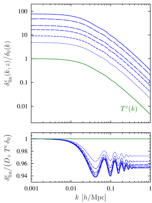
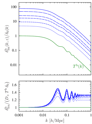
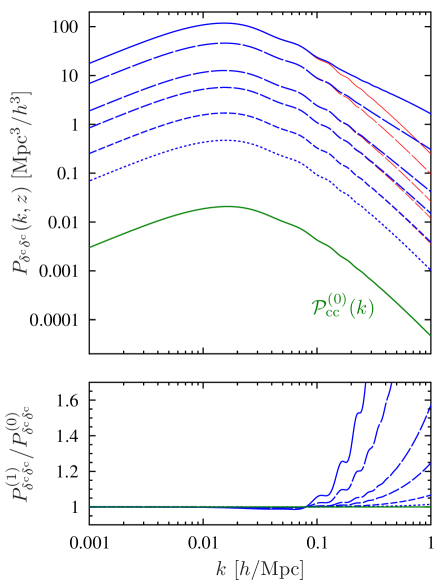
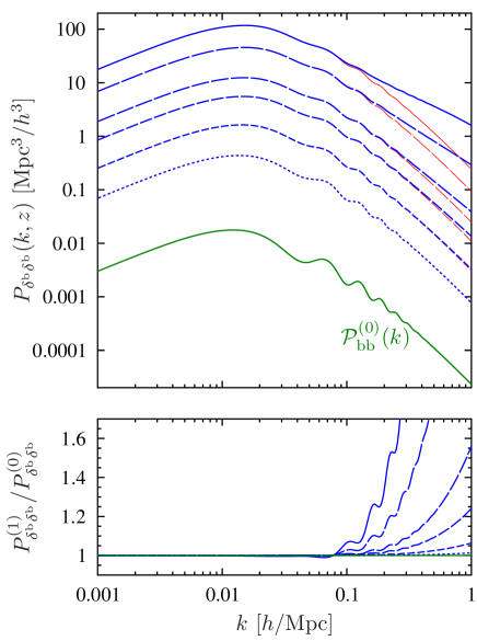
Figure 2: Evolution of the initial density perturbations for the CDM and baryons under the linear propagator, relative to the primordial density perturbation, as a function of spatial wavenumber and redshift. Top left and right panels: evolution of the CDM perturbations δcsuperscript𝛿c\delta^{\mathrm{c}}, and baryons, δbsuperscript𝛿b\delta^{\mathrm{b}}, respectively. Going from top to bottom, the blue solid through to dashed lines show results for redshifts z={0,1.0,3.0,5.0,10.0,20.0}𝑧01.03.05.010.020.0z=\{0,1.0,3.0,5.0,10.0,20.0\}. The solid green line at the bottom shows the initial mode. Bottom left and right panels: ratio of the linearly evolved CDM and baryon perturbations to the initial perturbations evolved under the standard linear growth factor for matter perturbations. Line styles are as for above.

The implicit solution for Ψa(𝐤,η)subscriptΨ𝑎𝐤𝜂\Psi_{a}({\bf k},\eta), Eq. (45), can be linearized, and the zeroth order term can be written: Ψa(0)(𝐤,η)=gab(η)ϕb(0)(𝐤)superscriptsubscriptΨ𝑎0𝐤𝜂subscript𝑔𝑎𝑏𝜂subscriptsuperscriptitalic-ϕ0𝑏𝐤\Psi_{a}^{(0)}({\bf k},\eta)=g_{ab}(\eta)\phi^{(0)}_{b}({\bf k}) (c.f. Eq. (88)). Following our discussions in §I and §II.5, we are interested in the case where the initial conditions are those of the post-recombination era Universe. Prior to this time, electrons and photons are tightly coupled through Thompson scattering, and photons drag electrons and baryons out of the potential wells. Thus at the end of recombination, baryons and dark matter are spatially displaced from one another (c.f. Fig. 1). In a somewhat simplified view, once the scattering processes are switched off, the evolution of the fluids can be captured by the two perturbations relaxing under gravity and so the evolving fields are simply some linear combination of the initial fields, with appropriate weight factors.

Fig. 2 graphically demonstrates this. Here we show the ratio of the initial CDM (left panel) and baryon (right panel) perturbations evolving under the action of the linear propagator gab(η)subscript𝑔𝑎𝑏𝜂g_{ab}(\eta), divided through by the amplitude of the initial primordial density perturbation that sourced them. For large-scale growing mode initial conditions (ua=ua(1))subscript𝑢𝑎superscriptsubscript𝑢𝑎1(u_{a}=u_{a}^{(1)}), then we have:

δlinc(𝐤,η)/δ0(k)=Ψ1(0)(𝐤,η)/δ0(k)subscriptsuperscript𝛿clin𝐤𝜂subscript𝛿0𝑘subscriptsuperscriptΨ01𝐤𝜂subscript𝛿0𝑘\displaystyle\delta^{\mathrm{c}}_{\mathrm{lin}}({\bf k},\eta)/\delta_{0}(k)=\Psi^{(0)}_{1}({\bf k},\eta)/\delta_{0}(k) =\displaystyle= [g11(η)+g12(η)]Tc(k)+[g13(η)+g14(η)]Tb(k)delimited-[]subscript𝑔11𝜂subscript𝑔12𝜂superscript𝑇c𝑘delimited-[]subscript𝑔13𝜂subscript𝑔14𝜂superscript𝑇b𝑘\displaystyle\left[g_{11}(\eta)+g_{12}(\eta)\right]T^{\mathrm{c}}(k)+\left[g_{13}(\eta)+g_{14}(\eta)\right]T^{\mathrm{b}}(k)\ (79)
=\displaystyle= [(1fb)eη+3fb(12eη/2)]Tc(k)+fb[eη3+2eη/2]Tb(k);delimited-[]1superscript𝑓bsuperscripte𝜂3superscript𝑓b12superscripte𝜂2superscript𝑇c𝑘superscript𝑓bdelimited-[]superscripte𝜂32superscripte𝜂2superscript𝑇b𝑘\displaystyle\left[(1-f^{\rm b}){\mathrm{e}}^{\eta}+3f^{\rm b}(1-2{\mathrm{e}}^{-\eta/2})\right]T^{\mathrm{c}}(k)+f^{\rm b}\left[{\mathrm{e}}^{\eta}-3+2{\mathrm{e}}^{-\eta/2}\right]T^{\mathrm{b}}(k)\ ;
δlinb(𝐤,η)/δ0(k)=Ψ3(0)(𝐤,η)/δ0(k)subscriptsuperscript𝛿blin𝐤𝜂subscript𝛿0𝑘subscriptsuperscriptΨ03𝐤𝜂subscript𝛿0𝑘\displaystyle\delta^{\mathrm{b}}_{\mathrm{lin}}({\bf k},\eta)/\delta_{0}(k)=\Psi^{(0)}_{3}({\bf k},\eta)/\delta_{0}(k) =\displaystyle= [g31(η)+g32(η)]Tc(k)+[g33(η)+g34(η)]Tb(k)delimited-[]subscript𝑔31𝜂subscript𝑔32𝜂superscript𝑇c𝑘delimited-[]subscript𝑔33𝜂subscript𝑔34𝜂superscript𝑇b𝑘\displaystyle\left[g_{31}(\eta)+g_{32}(\eta)\right]T^{\mathrm{c}}(k)+\left[g_{33}(\eta)+g_{34}(\eta)\right]T^{\mathrm{b}}(k)\ (80)
=\displaystyle= (1fb)[eη3+2eη/2]Tc(k)+[fbeη+(1fb)(32eη/2)]Tb(k).1superscript𝑓bdelimited-[]superscripte𝜂32superscripte𝜂2superscript𝑇c𝑘delimited-[]superscript𝑓bsuperscripte𝜂1superscript𝑓b32superscripte𝜂2superscript𝑇b𝑘\displaystyle(1-f^{\rm b})\left[{\mathrm{e}}^{\eta}-3+2{\mathrm{e}}^{-\eta/2}\right]T^{\mathrm{c}}(k)+\left[f^{\rm b}{\mathrm{e}}^{\eta}+(1-f^{\rm b})(3-2{\mathrm{e}}^{-\eta/2})\right]T^{\mathrm{b}}(k)\ .

In the limit of small and large η𝜂\eta these relations simplify to:

δlinc(𝐤,η)/δ0(k)subscriptsuperscript𝛿clin𝐤𝜂subscript𝛿0𝑘\displaystyle\delta^{\mathrm{c}}_{\mathrm{lin}}({\bf k},\eta)/\delta_{0}(k) \displaystyle\approx {Tc(k)(η1)eη[(1fb)Tc(k)+fbTb(k)](η1);casessuperscript𝑇c𝑘much-less-than𝜂1superscripte𝜂delimited-[]1superscript𝑓bsuperscript𝑇c𝑘superscript𝑓bsuperscript𝑇b𝑘much-greater-than𝜂1\displaystyle\left\{\begin{array}[]{ll}T^{\mathrm{c}}(k)&\quad(\eta\ll 1)\\ {\mathrm{e}}^{\eta}\left[(1-f^{\rm b})T^{\mathrm{c}}(k)+f^{\rm b}T^{\mathrm{b}}(k)\right]&\quad(\eta\gg 1)\end{array}\right.\ ; (83)
δlinb(𝐤,η)/δ0(k)subscriptsuperscript𝛿blin𝐤𝜂subscript𝛿0𝑘\displaystyle\delta^{\mathrm{b}}_{\mathrm{lin}}({\bf k},\eta)/\delta_{0}(k) \displaystyle\approx {Tb(k)(η1)eη[(1fb)Tc(k)+fbTb(k)](η1),casessuperscript𝑇b𝑘much-less-than𝜂1superscripte𝜂delimited-[]1superscript𝑓bsuperscript𝑇c𝑘superscript𝑓bsuperscript𝑇b𝑘much-greater-than𝜂1\displaystyle\left\{\begin{array}[]{ll}T^{\mathrm{b}}(k)&\quad(\eta\ll 1)\\ {\mathrm{e}}^{\eta}\left[(1-f^{\rm b})T^{\mathrm{c}}(k)+f^{\rm b}T^{\mathrm{b}}(k)\right]&\quad(\eta\gg 1)\end{array}\right.\ , (86)

where the η1much-greater-than𝜂1\eta\gg 1 relations, show that the fields evolve to an equilibrium state.

On inspecting Fig. 2, we note that on large scales at the initial time (green solid lines) the two perturbations are perfectly correlated with the primordial fluctuation. On smaller scales we see that both the CDM and baryon modes are damped, and this is due to the Mészáros effect (see Peebles, 1980; Dodelson, 2003). Also the waves have an oscillating structure as a function of k𝑘k, these are the Baryon Acoustic Oscillations (BAO) (for a discussion see Eisenstein and Hu, 1998; Meiksin et al., 1999). We also note that the BAO are almost absent in the dark matter distribution at zi=100subscript𝑧𝑖100z_{i}=100, whereas for the baryons they are strongly present.

As the system evolves linearly under gravity, we now see that on large scales (k<0.01hMpc1𝑘0.01superscriptMpc1k<0.01\,h\,{\rm Mpc}^{-1}) both solutions scale with time in accordance with the standard linear growth factor for the total matter perturbation on large scales: i.e., δm(k,η)=limk0[w1δc(k,η)+w2δb(k,η)]=D+(η)δm(k,η0)superscript𝛿mk𝜂subscript𝑘0delimited-[]subscript𝑤1superscript𝛿ck𝜂subscript𝑤2superscript𝛿bk𝜂subscript𝐷𝜂superscript𝛿mksubscript𝜂0\delta^{\mathrm{m}}(\hbox{\bf k},\eta)=\lim_{k\rightarrow 0}[w_{1}\delta^{\mathrm{c}}(\hbox{\bf k},\eta)+w_{2}\delta^{\mathrm{b}}(\hbox{\bf k},\eta)]=D_{+}(\eta)\delta^{\mathrm{m}}(\hbox{\bf k},\eta_{0}), which we obtain using the model of Carroll et al. (1992) with Ωm=Ωc+ΩbsubscriptΩmsubscriptΩcsubscriptΩb\Omega_{\mathrm{m}}=\Omega_{\mathrm{c}}+\Omega_{\mathrm{b}}. On smaller scales (k>0.01hMpc1𝑘0.01superscriptMpc1k>0.01\,h\,{\rm Mpc}^{-1}) the fluctuations grow with time, but now we note that the BAO features present in the baryon modes become damped, whilst those in the CDM grow. This can be seen more clearly by dividing each mode by D+(η)δ(0)(k)=D+(η)T(k)δ0(k)subscript𝐷𝜂superscript𝛿0𝑘subscript𝐷𝜂𝑇𝑘subscript𝛿0𝑘D_{+}(\eta)\delta^{(0)}(k)=D_{+}(\eta)T(k)\delta_{0}(k), for each component and this is what is plotted in the bottom panels of Fig. 2. Again, in the large scale limit, all Ti(k)1subscript𝑇𝑖𝑘1T_{i}(k)\rightarrow 1, and so g1b(η)ub(1)D+(η)subscript𝑔1𝑏𝜂subscriptsuperscript𝑢1𝑏subscript𝐷𝜂g_{1b}(\eta)u^{(1)}_{b}\rightarrow D_{+}(\eta). Hence δlinc(k,η)/[D+(η)Tc(k)δ0(k)]1subscriptsuperscript𝛿clin𝑘𝜂delimited-[]subscript𝐷𝜂superscript𝑇c𝑘subscript𝛿0𝑘1\delta^{\mathrm{c}}_{\mathrm{lin}}(k,\eta)/[D_{+}(\eta)T^{\mathrm{c}}(k)\delta_{0}(k)]\rightarrow 1, and likewise for the baryons. Thus we see that the amplitude of the BAO in the CDM are indeed increasing, and those in the baryons are decaying.

Note that for the CDM distribution, by z=5𝑧5z=5 the BAO are almost fully in place with <1%absentpercent1<1\% changes to the oscillation amplitude as the distribution is evolved to z=0𝑧0z=0. However between z=10𝑧10z=10 and 555 there is a significant difference and one must be careful to account for these changes when modeling BAO at high redshift. We now draw attention to the important fact that the baryon distributions display more significant changes, there being an almost 50% difference between the initial and final distributions on large-scales. As noted this will lead to significant baryon bias for statistical probes that are sensitive primarily to the distribution of baryons in the Universe and not the dark matter. In the following sections, we explore how non-linear evolution changes these results.

III Perturbation theory

III.1 Solutions

Following (Crocce and Scoccimarro, 2006a) we look for power series solutions to the equations of motion, Eq. (17)

Ψa(k,η)=j=0Ψa(j)(k,η)subscriptΨ𝑎k𝜂superscriptsubscript𝑗0subscriptsuperscriptΨ𝑗𝑎k𝜂\Psi_{a}(\hbox{\bf k},\eta)=\sum_{j=0}^{\infty}\Psi^{(j)}_{a}(\hbox{\bf k},\eta)\ (87)

(in our notation the linear solution is Ψ(0)superscriptΨ0\Psi^{(0)} as opposed to the more usual Ψ(1)superscriptΨ1\Psi^{(1)}). On inserting the above expression into the general solution of Eq. (45), we find that

Ψa(0)(k,η)subscriptsuperscriptΨ0𝑎k𝜂\displaystyle\Psi^{(0)}_{a}(\hbox{\bf k},\eta) =gab(η)ϕb(0)(k);absentsubscript𝑔𝑎𝑏𝜂subscriptsuperscriptitalic-ϕ0𝑏k\displaystyle=g_{ab}(\eta)\phi^{(0)}_{b}(\hbox{\bf k})\,; (88)
Ψa(1)(k,η)subscriptsuperscriptΨ1𝑎k𝜂\displaystyle\Psi^{(1)}_{a}(\hbox{\bf k},\eta) =0ηdηgab(ηη)γbcd(s)(k,k1,k2)Ψc(0)(k1,η)Ψd(0)(k2,η);absentsuperscriptsubscript0𝜂differential-dsuperscript𝜂subscript𝑔𝑎𝑏𝜂superscript𝜂subscriptsuperscript𝛾s𝑏𝑐𝑑ksubscriptk1subscriptk2superscriptsubscriptΨ𝑐0subscriptk1superscript𝜂superscriptsubscriptΨ𝑑0subscriptk2superscript𝜂\displaystyle=\int_{0}^{\eta}{\mathrm{d}}\eta^{\prime}g_{ab}(\eta-\eta^{\prime})\gamma^{\mathrm{(s)}}_{bcd}(\hbox{\bf k},\hbox{\bf k}_{1},\hbox{\bf k}_{2})\Psi_{c}^{(0)}(\hbox{\bf k}_{1},\eta^{\prime})\Psi_{d}^{(0)}(\hbox{\bf k}_{2},\eta^{\prime})\,; (89)
Ψa(2)(k,η)subscriptsuperscriptΨ2𝑎k𝜂\displaystyle\Psi^{(2)}_{a}(\hbox{\bf k},\eta) =20ηdηgab(ηη)γbcd(s)(k,k1,k2)Ψc(0)(k1,η)Ψd(1)(k2,η);absent2superscriptsubscript0𝜂differential-dsuperscript𝜂subscript𝑔𝑎𝑏𝜂superscript𝜂subscriptsuperscript𝛾s𝑏𝑐𝑑ksubscriptk1subscriptk2superscriptsubscriptΨ𝑐0subscriptk1superscript𝜂superscriptsubscriptΨ𝑑1subscriptk2superscript𝜂\displaystyle=2\int_{0}^{\eta}{\mathrm{d}}\eta^{\prime}g_{ab}(\eta-\eta^{\prime})\gamma^{\mathrm{(s)}}_{bcd}(\hbox{\bf k},\hbox{\bf k}_{1},\hbox{\bf k}_{2})\Psi_{c}^{(0)}(\hbox{\bf k}_{1},\eta^{\prime})\Psi_{d}^{(1)}(\hbox{\bf k}_{2},\eta^{\prime})\,; (90)
\displaystyle\vdots\hskip 28.45274pt \displaystyle\hskip 4.26773pt\vdots\hskip 56.9055pt\vdots\hskip 56.9055pt\vdots\hskip 56.9055pt\vdots
Ψa(n+1)(k,η)subscriptsuperscriptΨ𝑛1𝑎k𝜂\displaystyle\Psi^{(n+1)}_{a}(\hbox{\bf k},\eta) =0ηdηgab(ηη)γbcd(s)(k,k1,k2)m=0nΨc(nm)(k1,η)Ψd(m)(k2,η).absentsuperscriptsubscript0𝜂differential-dsuperscript𝜂subscript𝑔𝑎𝑏𝜂superscript𝜂subscriptsuperscript𝛾s𝑏𝑐𝑑ksubscriptk1subscriptk2superscriptsubscript𝑚0𝑛subscriptsuperscriptΨ𝑛𝑚𝑐subscriptk1superscript𝜂subscriptsuperscriptΨ𝑚𝑑subscriptk2superscript𝜂\displaystyle=\int_{0}^{\eta}{\mathrm{d}}\eta^{\prime}g_{ab}(\eta-\eta^{\prime})\gamma^{\mathrm{(s)}}_{bcd}(\hbox{\bf k},\hbox{\bf k}_{1},\hbox{\bf k}_{2})\sum_{m=0}^{n}\Psi^{(n-m)}_{c}(\hbox{\bf k}_{1},\eta^{\prime})\Psi^{(m)}_{d}(\hbox{\bf k}_{2},\eta^{\prime})\,. (91)

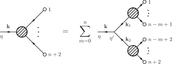
Fig. 3 shows a graphical representation of Eq. (91).

Refer to caption
Figure 3: Graphical representation of Eq. (91). The blob on the left hand side corresponds to Ψ(n+1)superscriptΨ𝑛1\Psi^{(n+1)} (which clearly involves n+2𝑛2n+2 initial conditions), while the two blobs on the right hand side correspond to Ψ(nm)superscriptΨ𝑛𝑚\Psi^{(n-m)} and Ψ(m)superscriptΨ𝑚\Psi^{(m)} (involving nm+1𝑛𝑚1n-m+1 and m+1𝑚1m+1 initial conditions) respectively. The trivalent vertex denotes the vertex matrix γ(s)superscript𝛾s\gamma^{\mathrm{(s)}}.

We may develop these solutions further by inserting into the above expressions the linear propagator gab(η)subscript𝑔𝑎𝑏𝜂g_{ab}(\eta) given by Eq. (48). Thus, for the linear evolution of the initial waves, we have:

Ψa(0)(k,η)=lelηgab,lϕb(0)(k).subscriptsuperscriptΨ0𝑎k𝜂subscript𝑙superscripte𝑙𝜂subscript𝑔𝑎𝑏𝑙subscriptsuperscriptitalic-ϕ0𝑏k\Psi^{(0)}_{a}(\hbox{\bf k},\eta)=\sum_{l}{\mathrm{e}}^{l\eta}g_{ab,l}\,\phi^{(0)}_{b}(\hbox{\bf k})\,. (92)

Similarly, for the first order solution we have

Ψa(1)(k,η)subscriptsuperscriptΨ1𝑎k𝜂\displaystyle\Psi^{(1)}_{a}(\hbox{\bf k},\eta) =\displaystyle= 0ηdηgab(ηη)γbcd(s)(k,k1,k2)gcc(η)ϕc(k1)gdd(η)ϕd(k2);superscriptsubscript0𝜂differential-dsuperscript𝜂subscript𝑔𝑎𝑏𝜂superscript𝜂subscriptsuperscript𝛾s𝑏𝑐𝑑ksubscriptk1subscriptk2subscript𝑔𝑐superscript𝑐superscript𝜂subscriptitalic-ϕsuperscript𝑐subscriptk1subscript𝑔𝑑superscript𝑑superscript𝜂subscriptitalic-ϕsuperscript𝑑subscriptk2\displaystyle\int_{0}^{\eta}{\mathrm{d}}\eta^{\prime}g_{ab}(\eta-\eta^{\prime})\gamma^{\mathrm{(s)}}_{bcd}(\hbox{\bf k},\hbox{\bf k}_{1},\hbox{\bf k}_{2})g_{cc^{\prime}}(\eta^{\prime})\phi_{c^{\prime}}(\hbox{\bf k}_{1})g_{dd^{\prime}}(\eta^{\prime})\phi_{d^{\prime}}(\hbox{\bf k}_{2})\ ; (93)
=\displaystyle= 0ηdηlel(ηη)gab,lγbcd(s)(k,k1,k2)memηgcc,mϕc(0)(k1)nenηgdd,nϕd(0)(k2)superscriptsubscript0𝜂differential-dsuperscript𝜂subscript𝑙superscripte𝑙𝜂superscript𝜂subscript𝑔𝑎𝑏𝑙subscriptsuperscript𝛾s𝑏𝑐𝑑ksubscriptk1subscriptk2subscript𝑚superscripte𝑚superscript𝜂subscript𝑔𝑐superscript𝑐𝑚subscriptsuperscriptitalic-ϕ0superscript𝑐subscriptk1subscript𝑛superscripte𝑛superscript𝜂subscript𝑔𝑑superscript𝑑𝑛subscriptsuperscriptitalic-ϕ0superscript𝑑subscriptk2\displaystyle\int_{0}^{\eta}{\mathrm{d}}\eta^{\prime}\sum_{l}{\mathrm{e}}^{l(\eta-\eta^{\prime})}g_{ab,l}\gamma^{\mathrm{(s)}}_{bcd}(\hbox{\bf k},\hbox{\bf k}_{1},\hbox{\bf k}_{2})\sum_{m}{\mathrm{e}}^{m\eta^{\prime}}g_{cc^{\prime},m}\,\phi^{(0)}_{c^{\prime}}(\hbox{\bf k}_{1})\sum_{n}{\mathrm{e}}^{n\eta^{\prime}}g_{dd^{\prime},n}\,\phi^{(0)}_{d^{\prime}}(\hbox{\bf k}_{2})
=\displaystyle= 0ηdηl,m,nelη+(m+nl)ηgab,lγbcd(s)(k,k1,k2)gcc,mgdd,nϕc(0)(k1)ϕd(0)(k2)superscriptsubscript0𝜂differential-dsuperscript𝜂subscript𝑙𝑚𝑛superscripte𝑙𝜂𝑚𝑛𝑙superscript𝜂subscript𝑔𝑎𝑏𝑙subscriptsuperscript𝛾s𝑏𝑐𝑑ksubscriptk1subscriptk2subscript𝑔𝑐superscript𝑐𝑚subscript𝑔𝑑superscript𝑑𝑛subscriptsuperscriptitalic-ϕ0superscript𝑐subscriptk1subscriptsuperscriptitalic-ϕ0superscript𝑑subscriptk2\displaystyle\int_{0}^{\eta}{\mathrm{d}}\eta^{\prime}\sum_{l,m,n}{\mathrm{e}}^{l\eta+(m+n-l)\eta^{\prime}}g_{ab,l}\gamma^{\mathrm{(s)}}_{bcd}(\hbox{\bf k},\hbox{\bf k}_{1},\hbox{\bf k}_{2})g_{cc^{\prime},m}\,g_{dd^{\prime},n}\,\phi^{(0)}_{c^{\prime}}(\hbox{\bf k}_{1})\phi^{(0)}_{d^{\prime}}(\hbox{\bf k}_{2})
=\displaystyle= l,m,nelηI1(m+nl;η)gab,lγ¯bcd(s)(k1,kk1)gcc,mgdd,nϕc(0)(k1)ϕd(0)(kk1),subscript𝑙𝑚𝑛superscripte𝑙𝜂subscript𝐼1𝑚𝑛𝑙𝜂subscript𝑔𝑎𝑏𝑙subscriptsuperscript¯𝛾s𝑏𝑐𝑑subscriptk1ksubscriptk1subscript𝑔𝑐superscript𝑐𝑚subscript𝑔𝑑superscript𝑑𝑛subscriptsuperscriptitalic-ϕ0superscript𝑐subscriptk1subscriptsuperscriptitalic-ϕ0superscript𝑑ksubscriptk1\displaystyle\sum_{l,m,n}{\mathrm{e}}^{l\eta}I_{1}(m+n-l;\eta)g_{ab,l}\,\bar{\gamma}^{\mathrm{(s)}}_{bcd}(\hbox{\bf k}_{1},\hbox{\bf k}-\hbox{\bf k}_{1})g_{cc^{\prime},m}\,g_{dd^{\prime},n}\,\phi^{(0)}_{c^{\prime}}(\hbox{\bf k}_{1})\phi^{(0)}_{d^{\prime}}(\hbox{\bf k}-\hbox{\bf k}_{1})\ ,

where in the last line we have introduced the function:

I1(l;η)=0ηdηelη={(elη1)/ll0ηl=0,subscript𝐼1𝑙𝜂superscriptsubscript0𝜂differential-dsuperscript𝜂superscripte𝑙superscript𝜂casessuperscripte𝑙𝜂1𝑙𝑙0𝜂𝑙0I_{1}(l;\eta)=\int_{0}^{\eta}{\mathrm{d}}\eta^{\prime}\,{\mathrm{e}}^{l\eta^{\prime}}=\left\{\begin{array}[]{ll}\displaystyle{({\mathrm{e}}^{l\eta}-1)/l}&l\neq 0\\ \eta&l=0\end{array}\right.\ , (94)

and performed the k2subscriptk2\hbox{\bf k}_{2} integral using the Dirac delta function implicit in γbcd(s)(k,k1,k2)subscriptsuperscript𝛾s𝑏𝑐𝑑ksubscriptk1subscriptk2\gamma^{\mathrm{(s)}}_{bcd}(\hbox{\bf k},\hbox{\bf k}_{1},\hbox{\bf k}_{2}).

In what follows we shall also need to make use of the 2nd order solution for the fields and after a similar procedure as above we find:

Ψa(2)(k,η)subscriptsuperscriptΨ2𝑎k𝜂\displaystyle\Psi^{(2)}_{a}(\hbox{\bf k},\eta) =\displaystyle= 2l,mp,q,relηI2(m+pl,q+rp;η)gab,lγ¯bcd(s)(k1,kk1)gcc,m2subscript𝑙𝑚subscript𝑝𝑞𝑟superscripte𝑙𝜂subscript𝐼2𝑚𝑝𝑙𝑞𝑟𝑝𝜂subscript𝑔𝑎𝑏𝑙subscriptsuperscript¯𝛾s𝑏𝑐𝑑subscriptk1ksubscriptk1subscript𝑔𝑐superscript𝑐𝑚\displaystyle 2\sum_{l,m}\sum_{p,q,r}{\mathrm{e}}^{l\eta}I_{2}(m+p-l,q+r-p;\eta)\,g_{ab,l}\,\bar{\gamma}^{\mathrm{(s)}}_{bcd}(\hbox{\bf k}_{1},\hbox{\bf k}-\hbox{\bf k}_{1})\,g_{cc^{\prime},m}\, (95)
×\displaystyle\times gdf,pγ¯fgh(s)(k2,kk1k2)ggg,qghh,rϕc(0)(k1)ϕg(0)(k2)ϕh(0)(kk1k2).subscript𝑔𝑑𝑓𝑝subscriptsuperscript¯𝛾s𝑓𝑔subscriptk2ksubscriptk1subscriptk2subscript𝑔𝑔superscript𝑔𝑞subscript𝑔superscript𝑟subscriptsuperscriptitalic-ϕ0superscript𝑐subscriptk1subscriptsuperscriptitalic-ϕ0superscript𝑔subscriptk2subscriptsuperscriptitalic-ϕ0superscriptksubscriptk1subscriptk2\displaystyle g_{df,p}\,\bar{\gamma}^{\mathrm{(s)}}_{fgh}(\hbox{\bf k}_{2},\hbox{\bf k}-\hbox{\bf k}_{1}-\hbox{\bf k}_{2})\,g_{gg^{\prime},q}\,g_{hh^{\prime},r}\,\phi^{(0)}_{c^{\prime}}(\hbox{\bf k}_{1})\phi^{(0)}_{g^{\prime}}(\hbox{\bf k}_{2})\phi^{(0)}_{h^{\prime}}(\hbox{\bf k}-\hbox{\bf k}_{1}-\hbox{\bf k}_{2})\ .

In the above we have introduced a further auxiliary function,

I2(l2,l1;η)=0ηdηel2ηI1(l1;η)={[l2e(l1+l2)η(l1+l2)el2η+l1]/[l1l2(l1+l2)](l10,l20)[el1η1l1η]/l12(l10,l2=0)[el2η(l2η1)+1]/l22(l1=0,l20)η2/2(l1=0,l2=0).subscript𝐼2subscript𝑙2subscript𝑙1𝜂superscriptsubscript0𝜂differential-d𝜂superscriptesubscript𝑙2superscript𝜂subscript𝐼1subscript𝑙1superscript𝜂casesdelimited-[]subscript𝑙2superscript𝑒subscript𝑙1subscript𝑙2𝜂subscript𝑙1subscript𝑙2superscript𝑒subscript𝑙2𝜂subscript𝑙1delimited-[]subscript𝑙1subscript𝑙2subscript𝑙1subscript𝑙2formulae-sequencesubscript𝑙10subscript𝑙20delimited-[]superscript𝑒subscript𝑙1𝜂1subscript𝑙1𝜂superscriptsubscript𝑙12formulae-sequencesubscript𝑙10subscript𝑙20delimited-[]superscript𝑒subscript𝑙2𝜂subscript𝑙2𝜂11superscriptsubscript𝑙22formulae-sequencesubscript𝑙10subscript𝑙20superscript𝜂22formulae-sequencesubscript𝑙10subscript𝑙20I_{2}(l_{2},l_{1};\eta)=\int_{0}^{\eta}{\mathrm{d}}\eta\,{\mathrm{e}}^{l_{2}\eta^{\prime}}I_{1}(l_{1};\eta^{\prime})\ =\left\{\begin{array}[]{ll}\left[l_{2}e^{(l_{1}+l_{2})\eta}-(l_{1}+l_{2})e^{l_{2}\eta}+l_{1}\right]/\left[l_{1}l_{2}(l_{1}+l_{2})\right]&(l_{1}\neq 0,l_{2}\neq 0)\\[2.15277pt] \left[e^{l_{1}\eta}-1-l_{1}\eta\right]/l_{1}^{2}&(l_{1}\neq 0,l_{2}=0)\\[2.15277pt] \left[e^{l_{2}\eta}(l_{2}\eta-1)+1\right]/l_{2}^{2}&(l_{1}=0,l_{2}\neq 0)\\[2.15277pt] \eta^{2}/2&(l_{1}=0,l_{2}=0)\end{array}\right.\ . (96)

III.2 Feynman rules for the PT solutions

As was shown by (Crocce and Scoccimarro, 2006a) there is a simple interpretation for the solutions Ψa(n)(𝐤)subscriptsuperscriptΨ𝑛𝑎𝐤\Psi^{(n)}_{a}({\bf k}) given by Eqs (88)–(91). The first equation in the hierarchy denotes an initial condition ϕa(0)superscriptsubscriptitalic-ϕ𝑎0\phi_{a}^{(0)}, evolved under the linear propagator gabsubscript𝑔𝑎𝑏g_{ab}. The second denotes the non-linear coupling between two initial waves of incoming momentum 𝐤1subscript𝐤1{\bf k}_{1} and 𝐤2subscript𝐤2{\bf k}_{2} through the interaction vertex γabc(s)(𝐤,𝐤1,𝐤2)subscriptsuperscript𝛾𝑠𝑎𝑏𝑐𝐤subscript𝐤1subscript𝐤2\gamma^{(s)}_{abc}({\bf k},{\bf k}_{1},{\bf k}_{2}), to produce an outgoing wave of momentum 𝐤=𝐤1+𝐤2𝐤subscript𝐤1subscript𝐤2{\bf k}={\bf k}_{1}+{\bf k}_{2}, which is one order higher in the PT series and evolving under the action of gabsubscript𝑔𝑎𝑏g_{ab}. For the next equation in the series we see that the solution structure is now repeated, and this recurs for all higher order terms. Thus a convenient graphical representation for the solutions is obtained by “iterating” the graph in Fig. 3, until on the right-hand-side we are left with diagrams involving only trivalent vertices and no “blobs”. Associated to this graphical representation is a simple set of Feynman rules for obtaining the n𝑛n-th order solution, Ψ(n)(k,η)superscriptΨ𝑛k𝜂\Psi^{(n)}(\hbox{\bf k},\eta); these may be stated as follows:

  1. 1.

    Draw all topologically distinct, connected tree diagrams containing n𝑛n vertices and a directed line coming into the diagram from the right for each of n+1𝑛1n+1 initial conditions, and a directed line going to the left out of the diagram for the final wave. Draw any number of directed internal lines running from one vertex to another, as required to give each vertex exactly two incoming and one outgoing attached line. It is most straightforward to label the direction of the lines by drawing arrows on them.

  2. 2.

    Assign each vertex its own time variable, sjsubscript𝑠𝑗s_{j}, and each line its own momentum, kjsubscriptk𝑗\hbox{\bf k}_{j}, such that momentum is conserved at each vertex, with the momenta considered to flow in the direction of the arrows. For the single outgoing line, assign the momentum k and final time η𝜂\eta.

  3. 3.

    Identify the various pieces of each diagram with the mathematical expressions as shown in Fig. 4.

  4. 4.

    Integrate over all intermediate times sjsubscript𝑠𝑗s_{j}, each between [0,η]0𝜂[0,\eta]. Integrate over all the independent wavevectors with the measure d3kjsuperscriptd3subscriptk𝑗{\mathrm{d}}^{3}\hbox{\bf k}_{j}. (Note that the momenta of all internal lines and a single incoming line are fixed by momentum conservation, thus there will be n𝑛n independent momenta to integrate over.) Sum over all internal field indices b𝑏b, c𝑐c, etc.

  5. 5.

    Each diagram carries a factor of 2rsuperscript2𝑟2^{r} if there are precisely r𝑟r vertices that are not symmetric with respect to interchanging their two incoming waves.

  6. 6.

    The value of Ψa(n)(k,η)superscriptsubscriptΨ𝑎𝑛k𝜂\Psi_{a}^{(n)}(\hbox{\bf k},\eta) is given by the sum over the values of these diagrams.

Refer to caption
Figure 4: Diagrammatic representation of the basic mathematical building blocks of the solutions. Left panel: the linear propagator gab(ηη)subscript𝑔𝑎𝑏𝜂superscript𝜂g_{ab}(\eta-\eta^{\prime}). Middle panel: the interaction vertex γ¯abc(s)(k1,k2)subscriptsuperscript¯𝛾s𝑎𝑏𝑐subscriptk1subscriptk2\bar{\gamma}^{\mathrm{(s)}}_{abc}(\hbox{\bf k}_{1},\hbox{\bf k}_{2}). The sticks are not part of the vertex and are present only to show the correct number of incoming and outgoing lines. Right panel: the initial field ϕa(0)(k)subscriptsuperscriptitalic-ϕ0𝑎k\phi^{(0)}_{a}(\hbox{\bf k}), denoted by the empty dot. The stick with the arrow serves only to show that an initial condition must always be connected to a diagram with a line going into the diagram, i.e. oriented away from the initial condition itself.

Fig. 5 shows all diagrams up to n=3𝑛3n=3, together with their symmetry factors calculated as in Step 5 above. As an example of the use of the Feynman rules, the expressions corresponding to the first two diagrams can be written,

Ψa(0)(k,η)subscriptsuperscriptΨ0𝑎k𝜂\displaystyle\Psi^{(0)}_{a}(\hbox{\bf k},\eta) =gab(η)ϕb(0)(k),absentsubscript𝑔𝑎𝑏𝜂subscriptsuperscriptitalic-ϕ0𝑏k\displaystyle=g_{ab}(\eta)\phi^{(0)}_{b}(\hbox{\bf k})\,, (97)
Ψa(1)(k,η)subscriptsuperscriptΨ1𝑎k𝜂\displaystyle\Psi^{(1)}_{a}(\hbox{\bf k},\eta) =0ηds1gab(ηs1)d3k1γ¯bcd(s)(k1,kk1)gcc(s1)ϕc(0)(k1)gdd(s1)ϕd(0)(kk1),absentsuperscriptsubscript0𝜂differential-dsubscript𝑠1subscript𝑔𝑎𝑏𝜂subscript𝑠1superscriptd3subscriptk1subscriptsuperscript¯𝛾s𝑏𝑐𝑑subscriptk1ksubscriptk1subscript𝑔𝑐superscript𝑐subscript𝑠1subscriptsuperscriptitalic-ϕ0superscript𝑐subscriptk1subscript𝑔𝑑superscript𝑑subscript𝑠1subscriptsuperscriptitalic-ϕ0superscript𝑑ksubscriptk1\displaystyle=\int_{0}^{\eta}{\mathrm{d}}s_{1}\,g_{ab}(\eta-s_{1})\int{\mathrm{d}}^{3}\hbox{\bf k}_{1}\,\bar{\gamma}^{\mathrm{(s)}}_{bcd}(\hbox{\bf k}_{1},\hbox{\bf k}-\hbox{\bf k}_{1})g_{cc^{\prime}}(s_{1})\phi^{(0)}_{c^{\prime}}(\hbox{\bf k}_{1})g_{dd^{\prime}}(s_{1})\phi^{(0)}_{d^{\prime}}(\hbox{\bf k}-\hbox{\bf k}_{1})\,, (98)

which are nothing but Eqs (92) and (93) (after performing the s1subscript𝑠1s_{1} integral in Eq. (98)). Similarly, evaluating the third diagram, we obtain Eq. (95), and so on.

Refer to caption
Figure 5: Graphical representation of the topologically distinct Feynman diagrams for the perturbation theory up to third order. From left to right we show, Ψa(n)(𝐤)superscriptsubscriptΨ𝑎𝑛𝐤\Psi_{a}^{(n)}({\bf k}), for n{0,1,2,3}𝑛0123n\in\{0,1,2,3\}, with the last two diagrams contributing to n=3𝑛3n=3.

IV Statistics

IV.1 Two-point covariance matrix of density and velocity modes

In cosmology rather than modeling Ψa(𝐤)subscriptΨ𝑎𝐤\Psi_{a}({\bf k}) at a particular point, we are more interested in computing statistical averages of various products of the fields at different points in space. We shall represent these statistical averages as: delimited-⟨⟩\left<\dots\right>. For mean zero fields, we must have Ψa(𝐤)=0delimited-⟨⟩subscriptΨ𝑎𝐤0\left<\Psi_{a}({\bf k})\right>=0. Thus the lowest order statistic of interest to us is the two-point correlation function, or power spectrum, of Ψa(𝐤)subscriptΨ𝑎𝐤\Psi_{a}({\bf k}), which can be defined:

Ψa(k,η)Ψb(k,η)=Pab(k,η)δD(k+k).delimited-⟨⟩subscriptΨ𝑎k𝜂subscriptΨ𝑏superscriptk𝜂subscript𝑃𝑎𝑏k𝜂superscript𝛿𝐷ksuperscriptk\left<\Psi_{a}(\hbox{\bf k},\eta)\Psi_{b}(\hbox{\bf k}^{\prime},\eta)\right\rangle=P_{ab}(\hbox{\bf k},\eta)\delta^{D}(\hbox{\bf k}+\hbox{\bf k}^{\prime})\,. (99)

IV.2 Two-point covariance matrix of initial fields

Throughout we will assume that the initial conditions are Gaussian. Consequently the statistical properties of the fields ϕa(0)(k)subscriptsuperscriptitalic-ϕ0𝑎k\phi^{(0)}_{a}(\hbox{\bf k}) are then completely characterized by the two-point covariance matrix:

ϕa(0)(k)ϕb(0)(k)𝒫ab(0)(k)δD(k+k).delimited-⟨⟩subscriptsuperscriptitalic-ϕ0𝑎ksubscriptsuperscriptitalic-ϕ0𝑏superscriptksubscriptsuperscript𝒫0𝑎𝑏𝑘superscript𝛿𝐷ksuperscriptk\left<\phi^{(0)}_{a}(\hbox{\bf k})\phi^{(0)}_{b}(\hbox{\bf k}^{\prime})\right>\equiv{\cal P}^{(0)}_{ab}(k)\delta^{D}(\hbox{\bf k}+\hbox{\bf k}^{\prime})\ . (100)

For the case of a CDM and baryon fluid this matrix takes the explicit form:

𝒫ab(0)(k)=[u12[Tc(k)]2u1u2[Tc(k)]2u1u3Tc(k)Tb(k)u1u4Tc(k)Tb(k)u1u2[Tc(k)]2u22[Tc(k)]2u2u3Tc(k)Tb(k)u2u4Tc(k)Tb(k)u1u3Tc(k)Tb(k)u2u3Tc(k)Tb(k)u32[Tb(k)]2u3u4[Tb(k)]2u1u4Tc(k)Tb(k)u2u4Tc(k)Tb(k)u3u4[Tb(k)]2u42[Tb(k)]2]𝒫0(k),subscriptsuperscript𝒫0𝑎𝑏𝑘delimited-[]superscriptsubscript𝑢12superscriptdelimited-[]superscript𝑇c𝑘2subscript𝑢1subscript𝑢2superscriptdelimited-[]superscript𝑇c𝑘2subscript𝑢1subscript𝑢3superscript𝑇c𝑘superscript𝑇b𝑘subscript𝑢1subscript𝑢4superscript𝑇c𝑘superscript𝑇b𝑘subscript𝑢1subscript𝑢2superscriptdelimited-[]superscript𝑇c𝑘2superscriptsubscript𝑢22superscriptdelimited-[]superscript𝑇c𝑘2subscript𝑢2subscript𝑢3superscript𝑇c𝑘superscript𝑇b𝑘subscript𝑢2subscript𝑢4superscript𝑇c𝑘superscript𝑇b𝑘subscript𝑢1subscript𝑢3superscript𝑇c𝑘superscript𝑇b𝑘subscript𝑢2subscript𝑢3superscript𝑇c𝑘superscript𝑇b𝑘superscriptsubscript𝑢32superscriptdelimited-[]superscript𝑇b𝑘2subscript𝑢3subscript𝑢4superscriptdelimited-[]superscript𝑇b𝑘2subscript𝑢1subscript𝑢4superscript𝑇c𝑘superscript𝑇b𝑘subscript𝑢2subscript𝑢4superscript𝑇c𝑘superscript𝑇b𝑘subscript𝑢3subscript𝑢4superscriptdelimited-[]superscript𝑇b𝑘2superscriptsubscript𝑢42superscriptdelimited-[]superscript𝑇b𝑘2subscript𝒫0𝑘{\cal P}^{(0)}_{ab}(k)=\left[\begin{array}[]{llll}u_{1}^{2}[T^{\mathrm{c}}(k)]^{2}&u_{1}u_{2}[T^{\mathrm{c}}(k)]^{2}&u_{1}u_{3}T^{\mathrm{c}}(k)T^{\mathrm{b}}(k)&u_{1}u_{4}T^{\mathrm{c}}(k)T^{\mathrm{b}}(k)\\ u_{1}u_{2}[T^{\mathrm{c}}(k)]^{2}&u_{2}^{2}[T^{\mathrm{c}}(k)]^{2}&u_{2}u_{3}T^{\mathrm{c}}(k)T^{\mathrm{b}}(k)&u_{2}u_{4}T^{\mathrm{c}}(k)T^{\mathrm{b}}(k)\\ u_{1}u_{3}T^{\mathrm{c}}(k)T^{\mathrm{b}}(k)&u_{2}u_{3}T^{\mathrm{c}}(k)T^{\mathrm{b}}(k)&u_{3}^{2}[T^{\mathrm{b}}(k)]^{2}&u_{3}u_{4}[T^{\mathrm{b}}(k)]^{2}\\ u_{1}u_{4}T^{\mathrm{c}}(k)T^{\mathrm{b}}(k)&u_{2}u_{4}T^{\mathrm{c}}(k)T^{\mathrm{b}}(k)&u_{3}u_{4}[T^{\mathrm{b}}(k)]^{2}&u_{4}^{2}[T^{\mathrm{b}}(k)]^{2}\end{array}\right]{\mathcal{P}}_{0}(k)\ , (101)

where we defined 𝒫0(k)δD(k+k)=δ0(k)δ0(k)subscript𝒫0𝑘superscript𝛿𝐷ksuperscriptkdelimited-⟨⟩subscript𝛿0ksubscript𝛿0superscriptk{\mathcal{P}}_{0}(k)\delta^{D}(\hbox{\bf k}+\hbox{\bf k}^{\prime})=\left<\delta_{0}(\hbox{\bf k})\delta_{0}(\hbox{\bf k}^{\prime})\right\rangle, to be the power spectrum of primordial density fluctuations: i.e. 𝒫0knproportional-tosubscript𝒫0superscript𝑘𝑛{\mathcal{P}}_{0}\propto k^{n}, with n=1𝑛1n=1 for the usual Harrison–Zel’dovich spectrum. The two-point correlation matrix of the initial fields may be expressed more compactly if we choose large-scale growing mode initial conditions, (ua=ua(1)=(1,1,1,1)subscript𝑢𝑎superscriptsubscript𝑢𝑎11111u_{a}=u_{a}^{(1)}=(1,1,1,1)), whereupon

𝒫ab(0)(k)=Ta(k)Tb(k)𝒫0(k),subscriptsuperscript𝒫0𝑎𝑏𝑘subscript𝑇𝑎𝑘subscript𝑇𝑏𝑘subscript𝒫0𝑘{\cal P}^{(0)}_{ab}(k)=T_{a}(k)T_{b}(k){\mathcal{P}}_{0}(k)\ , (102)

with [Ta(k)]T[Tc(k),Tc(k),Tb(k),Tb(k)]superscriptdelimited-[]subscript𝑇𝑎𝑘𝑇superscript𝑇c𝑘superscript𝑇c𝑘superscript𝑇b𝑘superscript𝑇b𝑘\left[T_{a}(k)\right]^{T}\equiv\left[T^{\mathrm{c}}(k),T^{\mathrm{c}}(k),T^{\mathrm{b}}(k),T^{\mathrm{b}}(k)\right].

For Gaussian initial conditions all of the multi-point correlators of the initial ϕa(0)(k)subscriptsuperscriptitalic-ϕ0𝑎k\phi^{(0)}_{a}(\hbox{\bf k}) can be computed using Wick’s theorem: all higher order correlators involving an odd number of fields vanish, while for an even number, there are (2n1)!!double-factorial2𝑛1(2n-1)!! contributions corresponding to the number of different pairings of the 2n2𝑛2n fields:

ϕa1(0)(k1)ϕa2n(0)(k2n)=all pair associationsp pairs of (i,j)ϕai(0)(ki)ϕaj(0)(kj).delimited-⟨⟩subscriptsuperscriptitalic-ϕ0subscript𝑎1subscriptk1subscriptsuperscriptitalic-ϕ0subscript𝑎2𝑛subscriptk2𝑛subscriptall pair associationssubscriptproductp pairs of 𝑖𝑗delimited-⟨⟩subscriptsuperscriptitalic-ϕ0subscript𝑎𝑖subscriptk𝑖subscriptsuperscriptitalic-ϕ0subscript𝑎𝑗subscriptk𝑗\left<\phi^{(0)}_{a_{1}}(\hbox{\bf k}_{1})\ldots\phi^{(0)}_{a_{2n}}(\hbox{\bf k}_{2n})\right\rangle=\sum_{\mbox{\scriptsize all pair associations}}\;\;\prod_{\mbox{\scriptsize p pairs of }(i,j)}\left<\phi^{(0)}_{a_{i}}(\hbox{\bf k}_{i})\phi^{(0)}_{a_{j}}(\hbox{\bf k}_{j})\right\rangle\,. (103)

For later use, we now also introduce a diagrammatic representation of the initial power spectrum matrix, see Fig. 6.

Refer to caption
Figure 6: Diagrammatic representation of the initial power spectrum matrix. The averaged pair of initial fields is denoted by the crossed dot, with the sticks and arrows serving only to show that each initial power spectrum will have two outgoing lines attached in any diagram.

IV.3 The non-linear propagator

As the non-linear interactions are turned on, the evolution of the initial field breaks away from the simple scaling, Ψa(𝐤,η)=gab(η)ϕb(0)(𝐤)subscriptΨ𝑎𝐤𝜂subscript𝑔𝑎𝑏𝜂subscriptsuperscriptitalic-ϕ0𝑏𝐤\Psi_{a}({\bf k},\eta)=g_{ab}(\eta)\phi^{(0)}_{b}({\bf k}). The deviations can be thought of as, erasing the memory of the mode to its initial conditions. This concept can be made more concrete, through introducing the non-linear propagator (Crocce and Scoccimarro, 2006a, b):

Gab(k,η)δD(kk)δΨa(k,η)[ϕ(0)]δϕb(0)(k).subscript𝐺𝑎𝑏k𝜂superscript𝛿𝐷ksuperscriptkdelimited-⟨⟩𝛿subscriptΨ𝑎k𝜂delimited-[]superscriptitalic-ϕ0𝛿superscriptsubscriptitalic-ϕ𝑏0superscriptkG_{ab}(\hbox{\bf k},\eta)\delta^{D}(\hbox{\bf k}-\hbox{\bf k}^{\prime})\equiv\left<\frac{\delta\Psi_{a}(\hbox{\bf k},\eta)[\phi^{(0)}]}{\delta\phi_{b}^{(0)}(\hbox{\bf k}^{\prime})}\right>\,. (104)

This means that we take the functional derivative of the full solution Ψa(k,η)subscriptΨ𝑎k𝜂\Psi_{a}(\hbox{\bf k},\eta) with respect to the initial condition ϕb(0)(k)subscriptsuperscriptitalic-ϕ0𝑏superscriptk\phi^{(0)}_{b}(\hbox{\bf k}^{\prime}), and then perform the ensemble average. Note that the non-linear propagator Gabsubscript𝐺𝑎𝑏G_{ab} is defined with the momentum conserving delta function factored out. The expectation is taken since, again, it is the average evolution of the mode away from its initial conditions that we are interested in.

In perturbation theory, the full solution is given as in Eq. (87), and thus

Gab(k,η)=l=0δGab(l)(k,η),subscript𝐺𝑎𝑏k𝜂superscriptsubscript𝑙0𝛿subscriptsuperscript𝐺𝑙𝑎𝑏k𝜂G_{ab}(\hbox{\bf k},\eta)=\sum_{l=0}^{\infty}\delta G^{(l)}_{ab}(\hbox{\bf k},\eta)\,, (105)

where

δGab(l)(k,η)δD(kk)=δΨa(2l)(k,η)[ϕ(0)]δϕb(0)(k).𝛿subscriptsuperscript𝐺𝑙𝑎𝑏k𝜂superscript𝛿𝐷ksuperscriptkdelimited-⟨⟩𝛿subscriptsuperscriptΨ2𝑙𝑎k𝜂delimited-[]superscriptitalic-ϕ0𝛿superscriptsubscriptitalic-ϕ𝑏0superscriptk\delta G^{(l)}_{ab}(\hbox{\bf k},\eta)\delta^{D}(\hbox{\bf k}-\hbox{\bf k}^{\prime})=\left<\frac{\delta\Psi^{(2l)}_{a}(\hbox{\bf k},\eta)[\phi^{(0)}]}{\delta\phi_{b}^{(0)}(\hbox{\bf k}^{\prime})}\right>\,. (106)

Notice that in the above equation we only consider contributions to the propagator that come from terms in the expansion of Ψa(𝐤,η)subscriptΨ𝑎𝐤𝜂\Psi_{a}({\bf k},\eta) with an odd number of initial conditions, i.e. only terms Ψa(j)(𝐤,η)subscriptsuperscriptΨ𝑗𝑎𝐤𝜂\Psi^{(j)}_{a}({\bf k},\eta) with j𝑗j an even number contribute. This owes to the fact that, for non-linear fields involving an even number of initial conditions, after performing the functional differentiation we are left with products that involve an isolated initial field, which vanishes on taking the expectation: ϕa(0)(𝐤)=0delimited-⟨⟩subscriptsuperscriptitalic-ϕ0𝑎𝐤0\langle\phi^{(0)}_{a}({\bf k})\rangle=0. Recall that we take j=0𝑗0j=0 as the first term in the perturbative series for ΨasubscriptΨ𝑎\Psi_{a}. Thus the total non-linear propagator up to one-loop level can be written:

Gab(1)(k,η)=gab(η)+δGab(1)(k,η),superscriptsubscript𝐺𝑎𝑏1k𝜂subscript𝑔𝑎𝑏𝜂𝛿subscriptsuperscript𝐺1𝑎𝑏k𝜂G_{ab}^{(1)}(\hbox{\bf k},\eta)=g_{ab}(\eta)+\delta G^{(1)}_{ab}(\hbox{\bf k},\eta)\ , (107)

where we used the fact that δGab(0)(k,η)=gab(η)𝛿superscriptsubscript𝐺𝑎𝑏0k𝜂subscript𝑔𝑎𝑏𝜂\delta G_{ab}^{(0)}(\hbox{\bf k},\eta)=g_{ab}(\eta), and where (Crocce and Scoccimarro, 2006b),

δGab(1)(𝐤,η)𝛿superscriptsubscript𝐺𝑎𝑏1𝐤𝜂\displaystyle\delta G_{ab}^{(1)}({\bf k},\eta) =\displaystyle= 40ηdη0ηdη′′gab(ηη)d3k1γ¯bcd(s)(𝐤1,𝐤𝐤1)gde(ηη′′)4superscriptsubscript0𝜂differential-dsuperscript𝜂superscriptsubscript0𝜂differential-dsuperscript𝜂′′subscript𝑔𝑎superscript𝑏𝜂superscript𝜂superscriptd3subscriptk1subscriptsuperscript¯𝛾ssuperscript𝑏𝑐𝑑subscript𝐤1𝐤subscript𝐤1subscript𝑔𝑑𝑒superscript𝜂superscript𝜂′′\displaystyle 4\int_{0}^{\eta}{\mathrm{d}}\eta^{\prime}\int_{0}^{\eta}{\mathrm{d}}\eta^{\prime\prime}g_{ab^{\prime}}(\eta-\eta^{\prime})\int{\mathrm{d}}^{3}\hbox{\bf k}_{1}\,\bar{\gamma}^{\mathrm{(s)}}_{b^{\prime}cd}({\bf k}_{1},{\bf k}-{\bf k}_{1})g_{de}(\eta^{\prime}-\eta^{\prime\prime}) (108)
×\displaystyle\times γ¯efg(s)(𝐤1,𝐤)gcc(η)gff(η′′)ggb(η′′)(𝐤1)𝒫cf(0)(k1).subscriptsuperscript¯𝛾s𝑒𝑓𝑔subscript𝐤1𝐤subscript𝑔𝑐superscript𝑐superscript𝜂subscript𝑔𝑓superscript𝑓superscript𝜂′′subscript𝑔𝑔𝑏superscript𝜂′′subscript𝐤1subscriptsuperscript𝒫0superscript𝑐superscript𝑓subscript𝑘1\displaystyle\bar{\gamma}^{\mathrm{(s)}}_{efg}(-{\bf k}_{1},{\bf k})g_{cc^{\prime}}(\eta^{\prime})g_{ff^{\prime}}(\eta^{\prime\prime})g_{gb}(\eta^{\prime\prime})({\bf k}_{1}){\cal P}^{(0)}_{c^{\prime}f^{\prime}}(k_{1})\ .

In Appendix B we present full details of the calculation for Eq. (106) explicitly for j=0,1,2𝑗012j=0,1,2.

As for the case of the perturbative solutions to ΨasubscriptΨ𝑎\Psi_{a}, the series expansion for the non-linear propagator with arbitrary numbers of loops can also be constructed in a diagrammatic fashion. Assuming Gaussian initial conditions, the Feynman rules for computing the n𝑛n-loop correction to the propagator, δGab(n)(k,η)𝛿subscriptsuperscript𝐺𝑛𝑎𝑏k𝜂\delta G^{(n)}_{ab}(\hbox{\bf k},\eta) are:

  1. 1.

    Draw all tree diagrams corresponding to Ψ(2n)(k,η)superscriptΨ2𝑛k𝜂\Psi^{(2n)}(\hbox{\bf k},\eta) as described in §III.2. Recall that these diagrams involve 2n+12𝑛12n+1 initial fields each.

  2. 2.

    For any specific tree, drop any one initial condition, labeling the incoming line thus created with the momentum k (this corresponds to the functional derivative and dropping the delta function). Pair the remaining 2n2𝑛2n initial fields in all possible ways into n𝑛n initial power spectra, as dictated by Wick’s theorem (corresponding to the ensemble averaging). Any specific tree then leads to (2n+1)(2n1)!!=(2n+1)!!2𝑛1double-factorial2𝑛1double-factorial2𝑛1(2n+1)(2n-1)!!=(2n+1)!! n𝑛n-loop diagrams, not all of which need to be topologically distinct. Diagrams containing a “tadpole” as a subdiagram (i.e. a subdiagram with a single external line) may be dropped, since they are zero, as explained below.

  3. 3.

    Follow Steps 24 of §III.2. When assigning the lines their momenta, ensure that the two lines emanating from an initial power spectrum carry equal and opposite momenta. Identify the various pieces of each diagram with the mathematical expressions as shown in Figs 4 and 6. (The number of independent momenta to integrate over in Step 4 will be just the number of independent loops, n𝑛n.)

  4. 4.

    Each diagram carries the appropriate factor of 2rsuperscript2𝑟2^{r} inherited form the original tree diagram. As noted above, it is possible that a specific loop diagram arises more than once. Of course such a diagram needs to be computed only once, but one must take account of its multiplicity explicitly.

  5. 5.

    The value of δGab(n)(k,η)𝛿subscriptsuperscript𝐺𝑛𝑎𝑏k𝜂\delta G^{(n)}_{ab}(\hbox{\bf k},\eta) is given by the sum over the values of all diagrams coming from all trees.

Fig. 7 shows all diagrams that arise in the computation of the one-loop propagator, including the symmetry factor computed in Step 4 above. Only the first two diagrams give non-vanishing contributions. The last diagram contains a tadpole (marked with the dashed box) and this gives zero contribution, since for each individual tadpole momentum conservation implies: α(k,k)=β(k,k)=0𝛼kk𝛽kk0\alpha(\hbox{\bf k},-\hbox{\bf k})=\beta(\hbox{\bf k},-\hbox{\bf k})=0. Hence, diagrams containing tadpoles vanish.

The power of the above graphical approach is that if one inspects the non-vanishing one-loop diagrams and uses the Feynman rules, then one can immediately write down the perturbative correction, as in Eq. (108).

Refer to caption
Figure 7: The diagrams for the one-loop non-linear propagator G(1)(k,η)superscript𝐺1k𝜂G^{(1)}(\hbox{\bf k},\eta). The first diagram represents Eq. (48); the second Eq. (108); and the last diagram contains a tadpole (marked with the dashed box) and thus evaluates to zero.

IV.4 Perturbative representation of the power spectrum

A perturbative expansion for the non-linear power spectrum may be obtained through insertion of the non-linear fields Ψa(n)superscriptsubscriptΨ𝑎𝑛\Psi_{a}^{(n)} (c.f. Eq. (91)) into Eq. (99), whereupon

Pab(k,η)=l=0δPab(l)(k,η).subscript𝑃𝑎𝑏k𝜂superscriptsubscript𝑙0𝛿superscriptsubscript𝑃𝑎𝑏𝑙k𝜂P_{ab}(\hbox{\bf k},\eta)=\sum_{l=0}^{\infty}\delta P_{ab}^{(l)}(\hbox{\bf k},\eta)\ . (109)

On assuming Gaussian initial conditions, then from Wick’s theorem we find that only those products of fields that involve an even number of initial conditions contribute to the non-linear power spectrum. Consequently we may write,

δPab(l)(k,η)δD(k+k)=j=02lΨa(j)(k,η)Ψb(2lj)(k,η).𝛿superscriptsubscript𝑃𝑎𝑏𝑙k𝜂superscript𝛿𝐷ksuperscriptksuperscriptsubscript𝑗02𝑙delimited-⟨⟩subscriptsuperscriptΨ𝑗𝑎k𝜂subscriptsuperscriptΨ2𝑙𝑗𝑏superscriptk𝜂\delta P_{ab}^{(l)}(\hbox{\bf k},\eta)\delta^{D}(\hbox{\bf k}+\hbox{\bf k}^{\prime})=\sum_{j=0}^{2l}\left<\Psi^{(j)}_{a}(\hbox{\bf k},\eta)\Psi^{(2l-j)}_{b}(\hbox{\bf k}^{\prime},\eta)\right\rangle\,. (110)

On taking all contributions to the power spectrum matrix up to one-loop, l=1𝑙1l=1, we have:

Pab=δPab(0)+δPab(1);subscript𝑃𝑎𝑏𝛿superscriptsubscript𝑃𝑎𝑏0𝛿superscriptsubscript𝑃𝑎𝑏1P_{ab}=\delta P_{ab}^{(0)}+\delta P_{ab}^{(1)}\ ; (111)

where the linear theory contribution (assuming large-scale growing mode initial conditions) is given by:

δPab(0)(k,η)δD(k+k)𝛿subscriptsuperscript𝑃0𝑎𝑏k𝜂superscript𝛿𝐷ksuperscriptk\displaystyle\delta P^{(0)}_{ab}(\hbox{\bf k},\eta)\delta^{D}(\hbox{\bf k}+\hbox{\bf k}^{\prime}) =\displaystyle= Ψa(0)(k,η)Ψb(0)(k,η)delimited-⟨⟩superscriptsubscriptΨ𝑎0k𝜂superscriptsubscriptΨ𝑏0superscriptk𝜂\displaystyle\left<\Psi_{a}^{(0)}(\hbox{\bf k},\eta)\Psi_{b}^{(0)}(\hbox{\bf k}^{\prime},\eta)\right>\ (112)
=\displaystyle= gaa(η)Ta(k)gbb(η)Tb(k)𝒫0(k)δD(k+k).subscript𝑔𝑎superscript𝑎𝜂subscript𝑇superscript𝑎𝑘subscript𝑔𝑏superscript𝑏𝜂subscript𝑇superscript𝑏𝑘subscript𝒫0𝑘superscript𝛿𝐷ksuperscriptk\displaystyle g_{aa^{\prime}}(\eta)T_{a^{\prime}}(k)g_{bb^{\prime}}(\eta)T_{b^{\prime}}(k){\mathcal{P}}_{0}(k)\delta^{D}(\hbox{\bf k}+\hbox{\bf k}^{\prime}).

We may also write the above expression using conventional matrix notation:

𝐏(0)(k,η)=𝐠(η)𝐓(k)𝐓T(k)𝐠T(η)𝒫0(k).superscript𝐏0k𝜂𝐠𝜂𝐓𝑘superscript𝐓𝑇𝑘superscript𝐠𝑇𝜂subscript𝒫0𝑘{\bf P}^{(0)}(\hbox{\bf k},\eta)={\bf g}(\eta){\bf T}(k){\bf T}^{T}(k){\bf g}^{T}(\eta){\mathcal{P}}_{0}(k)\,. (113)

The one-loop corrections to the power spectrum are written:

δPab(1)(k,η)δD(k+k)𝛿subscriptsuperscript𝑃1𝑎𝑏k𝜂superscript𝛿𝐷ksuperscriptk\displaystyle\delta P^{(1)}_{ab}(\hbox{\bf k},\eta)\delta^{D}(\hbox{\bf k}+\hbox{\bf k}^{\prime}) =\displaystyle= Ψa(0)(k,η)Ψb(2)(k,η)+Ψa(1)(k,η)Ψb(1)(k,η)+Ψa(2)(k,η)Ψb(0)(k,η).delimited-⟨⟩superscriptsubscriptΨ𝑎0k𝜂superscriptsubscriptΨ𝑏2superscriptk𝜂delimited-⟨⟩superscriptsubscriptΨ𝑎1k𝜂superscriptsubscriptΨ𝑏1superscriptk𝜂delimited-⟨⟩superscriptsubscriptΨ𝑎2k𝜂superscriptsubscriptΨ𝑏0superscriptk𝜂\displaystyle\left<\Psi_{a}^{(0)}(\hbox{\bf k},\eta)\Psi_{b}^{(2)}(\hbox{\bf k}^{\prime},\eta)\right>+\left<\Psi_{a}^{(1)}(\hbox{\bf k},\eta)\Psi_{b}^{(1)}(\hbox{\bf k}^{\prime},\eta)\right>+\left<\Psi_{a}^{(2)}(\hbox{\bf k},\eta)\Psi_{b}^{(0)}(\hbox{\bf k}^{\prime},\eta)\right>\ \,. (114)

Consider the sum of the first and last terms, we shall call these the “reducible” contributions and denote the sum of these terms: δPab,R(1)𝛿subscriptsuperscript𝑃1𝑎𝑏R\delta P^{(1)}_{ab,\mathrm{R}}. It was shown by (Crocce and Scoccimarro, 2006b) that the non-linear propagator plays the role of a Green’s function in the two-point sense, Ψaϕb(0)=Gacϕc(0)ϕb(0)delimited-⟨⟩subscriptΨ𝑎subscriptsuperscriptitalic-ϕ0𝑏subscript𝐺𝑎𝑐delimited-⟨⟩subscriptsuperscriptitalic-ϕ0𝑐subscriptsuperscriptitalic-ϕ0𝑏\langle\Psi_{a}\phi^{(0)}_{b}\rangle=G_{ac}\langle\phi^{(0)}_{c}\phi^{(0)}_{b}\rangle, and furthermore that this property holds order-by-order: Ψa(2n)ϕb(0)=δGac(n)ϕc(0)ϕb(0)delimited-⟨⟩subscriptsuperscriptΨ2𝑛𝑎subscriptsuperscriptitalic-ϕ0𝑏𝛿subscriptsuperscript𝐺𝑛𝑎𝑐delimited-⟨⟩subscriptsuperscriptitalic-ϕ0𝑐subscriptsuperscriptitalic-ϕ0𝑏\langle\Psi^{(2n)}_{a}\phi^{(0)}_{b}\rangle=\delta G^{(n)}_{ac}\langle\phi^{(0)}_{c}\phi^{(0)}_{b}\rangle. On applying the above relations, it is straightforward to see that we must have

δPab,R(1)(k,η)δD(k+k)𝛿subscriptsuperscript𝑃1𝑎𝑏Rk𝜂superscript𝛿𝐷ksuperscriptk\displaystyle\delta P^{(1)}_{ab,\mathrm{R}}(\hbox{\bf k},\eta)\delta^{D}(\hbox{\bf k}+\hbox{\bf k}^{\prime}) =\displaystyle= [Ψa(0)(k,η)Ψb(2)(k,η)+Ψa(2)(k,η)Ψb(0)(k,η)]delimited-[]delimited-⟨⟩superscriptsubscriptΨ𝑎0k𝜂superscriptsubscriptΨ𝑏2superscriptk𝜂delimited-⟨⟩superscriptsubscriptΨ𝑎2k𝜂superscriptsubscriptΨ𝑏0superscriptk𝜂\displaystyle\left[\left<\Psi_{a}^{(0)}(\hbox{\bf k},\eta)\Psi_{b}^{(2)}(\hbox{\bf k}^{\prime},\eta)\right>+\left<\Psi_{a}^{(2)}(\hbox{\bf k},\eta)\Psi_{b}^{(0)}(\hbox{\bf k}^{\prime},\eta)\right>\right] (115)
=\displaystyle= [gac(η)δGbd(1)(k,η)𝒫cd(0)(k)+δGac(1)(k,η)gbd(η)𝒫cd(0)(k)]δD(k+k).delimited-[]subscript𝑔𝑎𝑐𝜂𝛿subscriptsuperscript𝐺1𝑏𝑑superscriptk𝜂subscriptsuperscript𝒫0𝑐𝑑superscriptk𝛿subscriptsuperscript𝐺1𝑎𝑐k𝜂subscript𝑔𝑏𝑑𝜂subscriptsuperscript𝒫0𝑐𝑑ksuperscript𝛿𝐷ksuperscriptk\displaystyle\left[g_{ac}(\eta)\delta G^{(1)}_{bd}(\hbox{\bf k}^{\prime},\eta){\cal P}^{(0)}_{cd}(\hbox{\bf k}^{\prime})+\delta G^{(1)}_{ac}(\hbox{\bf k},\eta)g_{bd}(\eta){\cal P}^{(0)}_{cd}(\hbox{\bf k})\right]\delta^{D}(\hbox{\bf k}+\hbox{\bf k}^{\prime})\,.

Specializing to growing mode initial conditions, and using momentum conservation, we find

δPab,R(1)(k,η)=[gac(η)δGbd(1)(k,η)+δGac(1)(k,η)gbd(η)]Tc(k)Td(k)𝒫0(k).𝛿subscriptsuperscript𝑃1𝑎𝑏Rk𝜂delimited-[]subscript𝑔𝑎𝑐𝜂𝛿subscriptsuperscript𝐺1𝑏𝑑k𝜂𝛿subscriptsuperscript𝐺1𝑎𝑐k𝜂subscript𝑔𝑏𝑑𝜂subscript𝑇𝑐𝑘subscript𝑇𝑑𝑘subscript𝒫0𝑘\delta P^{(1)}_{ab,\mathrm{R}}(\hbox{\bf k},\eta)=\left[g_{ac}(\eta)\delta G^{(1)}_{bd}(\hbox{\bf k},\eta)+\delta G^{(1)}_{ac}(\hbox{\bf k},\eta)g_{bd}(\eta)\right]T_{c}(k)T_{d}(k){\mathcal{P}}_{0}(k)\,. (116)

In particular, we can write this in conventional matrix notation as

δ𝐏R(1)(k,η)=[𝐠(η)𝐓(k)𝐓T(k)[δ𝐆(1)]T(k,η)+δ𝐆(1)(k,η)𝐓(k)𝐓T(k)𝐠T(η)]𝒫0(k).𝛿subscriptsuperscript𝐏1Rk𝜂delimited-[]𝐠𝜂𝐓𝑘superscript𝐓𝑇𝑘superscriptdelimited-[]𝛿superscript𝐆1𝑇k𝜂𝛿superscript𝐆1k𝜂𝐓𝑘superscript𝐓𝑇𝑘superscript𝐠𝑇𝜂subscript𝒫0𝑘\delta{\bf P}^{(1)}_{\mathrm{R}}(\hbox{\bf k},\eta)=\left[{\bf g}(\eta){\bf T}(k){\bf T}^{T}(k)\big{[}\delta{\bf G}^{(1)}\big{]}^{T}(\hbox{\bf k},\eta)+\delta{\bf G}^{(1)}(\hbox{\bf k},\eta){\bf T}(k){\bf T}^{T}(k){\bf g}^{T}(\eta)\right]{\mathcal{P}}_{0}(k)\,. (117)

Adding Eqs (113) and (117), we see that the sum [𝐏(0)(k,η)+δ𝐏R(1)(k,η)]delimited-[]superscript𝐏0k𝜂𝛿subscriptsuperscript𝐏1Rk𝜂\big{[}{\bf P}^{(0)}(\hbox{\bf k},\eta)+\delta{\bf P}^{(1)}_{\mathrm{R}}(\hbox{\bf k},\eta)\big{]} is nothing but the one-loop truncation of the all-order expression

𝐏R(k,η)=𝐆(k,η)𝐓(k)𝐓T(k)𝐆T(k,η)𝒫0(k).subscript𝐏Rk𝜂𝐆k𝜂𝐓𝑘superscript𝐓𝑇𝑘superscript𝐆𝑇k𝜂subscript𝒫0𝑘{\bf P}_{\mathrm{R}}(\hbox{\bf k},\eta)={\bf G}(\hbox{\bf k},\eta){\bf T}(k){\bf T}^{T}(k){\bf G}^{T}(\hbox{\bf k},\eta){\cal P}_{0}(k)\,. (118)

The all-order reducible contribution collects all corrections to 𝐏(k,η)𝐏k𝜂{\bf P}(\hbox{\bf k},\eta) that are proportional to the initial power spectrum at the same scale k𝑘k.

Turning now to the second term in Eq. (114), conventionally called the “mode-coupling” contribution, we find that it can be written (Crocce and Scoccimarro, 2006a):

δPab,MC(1)(k,η)=20ηdη0ηdη′′d3k1gac(ηη)γ¯cde(s)(k1,kk1)gdd(η)gee(η)×gbf(ηη′′)γ¯fgh(s)(k1,k1k)ggg(η′′)ghh(η′′)𝒫dg(0)(k1)𝒫eh(0)(|kk1|).𝛿subscriptsuperscript𝑃1𝑎𝑏MCk𝜂2superscriptsubscript0𝜂differential-dsuperscript𝜂superscriptsubscript0𝜂differential-dsuperscript𝜂′′superscriptd3subscriptk1subscript𝑔𝑎𝑐𝜂superscript𝜂subscriptsuperscript¯𝛾s𝑐𝑑𝑒subscriptk1ksubscriptk1subscript𝑔𝑑superscript𝑑superscript𝜂subscript𝑔𝑒superscript𝑒superscript𝜂subscript𝑔𝑏𝑓𝜂superscript𝜂′′subscriptsuperscript¯𝛾s𝑓𝑔subscriptk1subscriptk1ksubscript𝑔𝑔superscript𝑔superscript𝜂′′subscript𝑔superscriptsuperscript𝜂′′subscriptsuperscript𝒫0superscript𝑑superscript𝑔subscript𝑘1subscriptsuperscript𝒫0superscript𝑒superscriptksubscriptk1\begin{split}\delta P^{(1)}_{ab,\mathrm{MC}}(\hbox{\bf k},\eta)&=2\int_{0}^{\eta}{\mathrm{d}}\eta^{\prime}\int_{0}^{\eta}{\mathrm{d}}\eta^{\prime\prime}\int{\mathrm{d}}^{3}\hbox{\bf k}_{1}\,g_{ac}(\eta-\eta^{\prime})\bar{\gamma}^{\mathrm{(s)}}_{cde}(\hbox{\bf k}_{1},\hbox{\bf k}-\hbox{\bf k}_{1})g_{dd^{\prime}}(\eta^{\prime})g_{ee^{\prime}}(\eta^{\prime})\\ &\quad\times g_{bf}(\eta-\eta^{\prime\prime})\bar{\gamma}^{\mathrm{(s)}}_{fgh}(-\hbox{\bf k}_{1},\hbox{\bf k}_{1}-\hbox{\bf k})g_{gg^{\prime}}(\eta^{\prime\prime})g_{hh^{\prime}}(\eta^{\prime\prime}){\cal P}^{(0)}_{d^{\prime}g^{\prime}}(k_{1}){\cal P}^{(0)}_{e^{\prime}h^{\prime}}(|\hbox{\bf k}-\hbox{\bf k}_{1}|)\,.\end{split} (119)

The mode-coupling piece includes corrections coming from modes other than k𝑘k in the initial power spectrum. In particular, we see from Eq. (119) that the one-loop mode-coupling correction involves the convolution of two initial power spectra with a specific kernel. At higher loop orders, the mode-coupling pieces involve convolutions of more than two initial powers.

The upshot is that for growing mode initial conditions, we can write the full power spectrum as

𝐏(k,η)=𝐆(k,η)𝐓(k)𝐓T(k)𝐆T(k,η)𝒫0(k)+𝐏MC(k,η).𝐏k𝜂𝐆k𝜂𝐓𝑘superscript𝐓𝑇𝑘superscript𝐆𝑇k𝜂subscript𝒫0𝑘subscript𝐏MCk𝜂{\bf P}(\hbox{\bf k},\eta)={\bf G}(\hbox{\bf k},\eta){\bf T}(k){\bf T}^{T}(k){\bf G}^{T}(\hbox{\bf k},\eta){\mathcal{P}}_{0}(k)+{\bf P}_{\mathrm{MC}}(\hbox{\bf k},\eta)\,. (120)

At this point we may extend our diagrammatic description: assuming Gaussian initial conditions, the Feynman rules for computing the n𝑛n-loop correction to the power spectrum, δPab(n)(k,η)𝛿subscriptsuperscript𝑃𝑛𝑎𝑏k𝜂\delta P^{(n)}_{ab}(\hbox{\bf k},\eta) are:

  1. 1.

    Draw the sum of all tree diagrams corresponding to Ψ(j)(k,η)superscriptΨ𝑗k𝜂\Psi^{(j)}(\hbox{\bf k},\eta), and the sum of diagrams corresponding to Ψ(2nj)(k,η)superscriptΨ2𝑛𝑗superscriptk𝜂\Psi^{(2n-j)}(\hbox{\bf k}^{\prime},\eta) as described in §III.2, including the arrows on the lines.

  2. 2.

    Formally “multiply” these two sums using distributivity. It is convenient to draw one set of diagrams flipped around the vertical axis, so that after the pairing of diagrams for Ψ(j)(k,η)superscriptΨ𝑗k𝜂\Psi^{(j)}(\hbox{\bf k},\eta) with those for Ψ(2nj)(k,η)superscriptΨ2𝑛𝑗k𝜂\Psi^{(2n-j)}(\hbox{\bf k},\eta), their initial conditions face each other. Next, pair the 2n+22𝑛22n+2 initial fields into n+1𝑛1n+1 initial power spectra (some pairings may lead to the same loop diagram). Disregard diagrams that contain a tadpole as a subdiagram. (This includes disconnected diagrams in particular.)

  3. 3.

    Follow Step 3 of §IV.3.

  4. 4.

    Each diagram carries the appropriate factor of 2r+ssuperscript2𝑟𝑠2^{r+s} inherited form the two original tree diagrams. As noted above, it is possible that a specific loop diagram arises more than once. Such a diagram needs to be computed only once, but its multiplicity must be taken into account.

  5. 5.

    The value of δPab(n)(k,η)𝛿subscriptsuperscript𝑃𝑛𝑎𝑏k𝜂\delta P^{(n)}_{ab}(\hbox{\bf k},\eta) is given by the sum over the the values of these diagrams for all j=0,,2n𝑗02𝑛j=0,\ldots,2n.

Fig. 8 shows all non-zero diagrams for the power spectrum up to one-loop order, including the symmetry factor computed in Step 4 above. In particular, notice how Eq. (115) is very simple to write down by inspecting the second and third graphs. The last diagram corresponds to the mode-coupling piece. Evidently Eq. (119) may be written down immediately by inspecting this graph.

Refer to caption
Figure 8: The non-zero diagrams for the one-loop power spectrum P(1)(k,η)superscript𝑃1k𝜂P^{(1)}(\hbox{\bf k},\eta). The dashed lines indicate the points at which the two trees were glued together. The first diagram represents Eq. (112); the second and third graphs are the two reducible contributions in Eq. (117); and the fourth graph represents the mode-coupling term of Eq. (119).

V One-loop corrections to the power spectrum

V.1 The non-linear propagator

In §IV, we defined the non-linear propagator Gab(𝐤,η)subscript𝐺𝑎𝑏𝐤𝜂G_{ab}({\bf k},\eta) as the ensemble average of the functional derivative of the full solution Ψa(k,η)subscriptΨ𝑎k𝜂\Psi_{a}(\hbox{\bf k},\eta) by the initial condition ϕb(0)(k)subscriptsuperscriptitalic-ϕ0𝑏superscriptk\phi^{(0)}_{b}(\hbox{\bf k}^{\prime}), without the delta function for momentum conservation (c.f. Eq. (104)). It was shown to have a perturbative expansion (c.f. Eqs (105) and (106)) and terms up to one-loop level were computed in Appendix B. Here we further develop the one-loop expression for the case of N=2𝑁2N=2 fluids.

To begin, let us reconsider Eq. (108), we may expand all of the linear propagators, gab(η)subscript𝑔𝑎𝑏𝜂g_{ab}(\eta), using Eq. (48) to obtain,

δGaa(1)(𝐤,η)𝛿subscriptsuperscript𝐺1𝑎superscript𝑎𝐤𝜂\displaystyle\delta G^{(1)}_{aa^{\prime}}({\bf k},\eta) =\displaystyle= 40ηdηl1gab,l1el1(ηη)d3𝐤1γ¯bcd(s)(𝐤1,𝐤𝐤1)l2gcc,l2el2η0ηdη′′l3gde,l3el3(ηη′′)4superscriptsubscript0𝜂differential-dsuperscript𝜂subscriptsubscript𝑙1subscript𝑔𝑎𝑏subscript𝑙1superscriptesubscript𝑙1𝜂superscript𝜂superscriptd3subscript𝐤1subscriptsuperscript¯𝛾𝑠𝑏𝑐𝑑subscript𝐤1𝐤subscript𝐤1subscriptsubscript𝑙2subscript𝑔𝑐superscript𝑐subscript𝑙2superscriptesubscript𝑙2superscript𝜂superscriptsubscript0superscript𝜂differential-dsuperscript𝜂′′subscriptsubscript𝑙3subscript𝑔𝑑𝑒subscript𝑙3superscriptesubscript𝑙3superscript𝜂superscript𝜂′′\displaystyle 4\int_{0}^{\eta}{\mathrm{d}}\eta^{\prime}\sum_{l_{1}}g_{ab,l_{1}}{\mathrm{e}}^{l_{1}(\eta-\eta^{\prime})}\int{\mathrm{d}}^{3}{\bf k}_{1}\bar{\gamma}^{(s)}_{bcd}({\bf k}_{1},{\bf k}-{\bf k}_{1})\sum_{l_{2}}g_{cc^{\prime},l_{2}}{\mathrm{e}}^{l_{2}\eta^{\prime}}\int_{0}^{\eta^{\prime}}{\mathrm{d}}\eta^{\prime\prime}\sum_{l_{3}}g_{de,l_{3}}{\mathrm{e}}^{l_{3}(\eta^{\prime}-\eta^{\prime\prime})} (121)
×\displaystyle\times γ¯efg(s)(𝐤1,𝐤)l4gff,l4el4η′′l5gga,l5el5η′′𝒫cf(0)(k1).subscriptsuperscript¯𝛾𝑠𝑒𝑓𝑔subscript𝐤1superscript𝐤subscriptsubscript𝑙4subscript𝑔𝑓superscript𝑓subscript𝑙4superscriptesubscript𝑙4superscript𝜂′′subscriptsubscript𝑙5subscript𝑔𝑔superscript𝑎subscript𝑙5superscriptesubscript𝑙5superscript𝜂′′superscriptsubscript𝒫superscript𝑐superscript𝑓0subscript𝑘1\displaystyle\bar{\gamma}^{(s)}_{efg}(-{\bf k}_{1},{\bf k}^{\prime})\sum_{l_{4}}g_{ff^{\prime},l_{4}}{\mathrm{e}}^{l_{4}\eta^{\prime\prime}}\sum_{l_{5}}g_{ga^{\prime},l_{5}}{\mathrm{e}}^{l_{5}\eta^{\prime\prime}}{\mathcal{P}}_{c^{\prime}f^{\prime}}^{(0)}(k_{1})\ .

On rearranging the above expression we find,

δGaa(1)(𝐤,η)𝛿subscriptsuperscript𝐺1𝑎superscript𝑎𝐤𝜂\displaystyle\delta G^{(1)}_{aa^{\prime}}({\bf k},\eta) =\displaystyle= 4l1,,l5el1η0ηdηe(l2+l3l1)η0ηdη′′e(l4+l5l3)η′′4subscriptsubscript𝑙1subscript𝑙5superscriptesubscript𝑙1𝜂superscriptsubscript0𝜂differential-dsuperscript𝜂superscriptesubscript𝑙2subscript𝑙3subscript𝑙1superscript𝜂superscriptsubscript0superscript𝜂differential-dsuperscript𝜂′′superscriptesubscript𝑙4subscript𝑙5subscript𝑙3superscript𝜂′′\displaystyle 4\sum_{l_{1},\dots,l_{5}}{\mathrm{e}}^{l_{1}\eta}\int_{0}^{\eta}{\mathrm{d}}\eta^{\prime}{\mathrm{e}}^{(l_{2}+l_{3}-l_{1})\eta^{\prime}}\int_{0}^{\eta^{\prime}}{\mathrm{d}}\eta^{\prime\prime}{\mathrm{e}}^{(l_{4}+l_{5}-l_{3})\eta^{\prime\prime}} (122)
×\displaystyle\times gab,l1d3𝐤1γ¯bcd(s)(𝐤1,𝐤𝐤1)gcc,l2gde,l3γ¯efg(s)(𝐤1,𝐤)gff,l4gga,l5𝒫cf(0)(k1).subscript𝑔𝑎𝑏subscript𝑙1superscriptd3subscript𝐤1subscriptsuperscript¯𝛾𝑠𝑏𝑐𝑑subscript𝐤1𝐤subscript𝐤1subscript𝑔𝑐superscript𝑐subscript𝑙2subscript𝑔𝑑𝑒subscript𝑙3subscriptsuperscript¯𝛾𝑠𝑒𝑓𝑔subscript𝐤1superscript𝐤subscript𝑔𝑓superscript𝑓subscript𝑙4subscript𝑔𝑔superscript𝑎subscript𝑙5superscriptsubscript𝒫superscript𝑐superscript𝑓0subscript𝑘1\displaystyle g_{ab,l_{1}}\,\int{\mathrm{d}}^{3}{\bf k}_{1}\bar{\gamma}^{(s)}_{bcd}({\bf k}_{1},{\bf k}-{\bf k}_{1})g_{cc^{\prime},l_{2}}\,g_{de,l_{3}}\,\bar{\gamma}^{(s)}_{efg}(-{\bf k}_{1},{\bf k}^{\prime})g_{ff^{\prime},l_{4}}\,g_{ga^{\prime},l_{5}}{\mathcal{P}}_{c^{\prime}f^{\prime}}^{(0)}(k_{1})\ .

Considering the integrals over ηsuperscript𝜂\eta^{\prime} and η′′superscript𝜂′′\eta^{\prime\prime}, these may be conveniently evaluated using the algebraic function I2(l2,l1,η)subscript𝐼2subscript𝑙2subscript𝑙1𝜂I_{2}(l_{2},l_{1},\eta) (c.f. Eq. (96)). Thus our final expression for the one-loop propagator takes the form:

δGaa(1)(k,η)𝛿subscriptsuperscript𝐺1𝑎superscript𝑎k𝜂\displaystyle\delta G^{(1)}_{aa^{\prime}}(\hbox{\bf k},\eta) =\displaystyle= 4l1,,l5elηI2(l2+l3l1,l4+l5l3;η)4subscriptsubscript𝑙1subscript𝑙5superscripte𝑙𝜂subscript𝐼2subscript𝑙2subscript𝑙3subscript𝑙1subscript𝑙4subscript𝑙5subscript𝑙3𝜂\displaystyle 4\sum_{l_{1},\dots,l_{5}}{\mathrm{e}}^{l\eta}I_{2}(l_{2}+l_{3}-l_{1},l_{4}+l_{5}-l_{3};\eta) (123)
×\displaystyle\times gab,l1d3𝐤1γ¯bcd(s)(k1,kk1)gcc,l2gde,l3γ¯efg(s)(k1,k)gff,l4gga,l5𝒫cf(0)(k1).subscript𝑔𝑎𝑏subscript𝑙1superscriptd3subscript𝐤1subscriptsuperscript¯𝛾s𝑏𝑐𝑑subscriptk1ksubscriptk1subscript𝑔𝑐superscript𝑐subscript𝑙2subscript𝑔𝑑𝑒subscript𝑙3subscriptsuperscript¯𝛾s𝑒𝑓𝑔subscriptk1ksubscript𝑔𝑓superscript𝑓subscript𝑙4subscript𝑔𝑔superscript𝑎subscript𝑙5superscriptsubscript𝒫superscript𝑐superscript𝑓0subscript𝑘1\displaystyle g_{ab,l_{1}}\int{\mathrm{d}}^{3}{\bf k}_{1}\,\bar{\gamma}^{\mathrm{(s)}}_{bcd}(\hbox{\bf k}_{1},\hbox{\bf k}-\hbox{\bf k}_{1})g_{cc^{\prime},l_{2}}\,g_{de,l_{3}}\bar{\gamma}^{\mathrm{(s)}}_{efg}(-\hbox{\bf k}_{1},\hbox{\bf k})g_{ff^{\prime},l_{4}}\,g_{ga^{\prime},l_{5}}\,{\mathcal{P}}_{c^{\prime}f^{\prime}}^{(0)}(k_{1})\ .

This expression may be reorganized so that the time dependent algebraic functions, the constant coefficient matrices gab,lsubscript𝑔𝑎𝑏𝑙g_{ab,l} and the k𝑘k-dependent matrices are grouped together. Further, if we take large-scale growing mode initial conditions, ua=ua(1)=(1,1,1,1)subscript𝑢𝑎superscriptsubscript𝑢𝑎11111u_{a}=u_{a}^{(1)}=(1,1,1,1), then we find that the propagator may be written,

δGaa(1)(k,η)𝛿subscriptsuperscript𝐺1𝑎superscript𝑎k𝜂\displaystyle\delta G^{(1)}_{aa^{\prime}}(\hbox{\bf k},\eta) =\displaystyle= 4l1,,l5elηI2(l2+l3l1,l4+l5l3;η)gab,l1gcc,l2gde,l3gff,l4gga,l54subscriptsubscript𝑙1subscript𝑙5superscripte𝑙𝜂subscript𝐼2subscript𝑙2subscript𝑙3subscript𝑙1subscript𝑙4subscript𝑙5subscript𝑙3𝜂subscript𝑔𝑎𝑏subscript𝑙1subscript𝑔𝑐superscript𝑐subscript𝑙2subscript𝑔𝑑𝑒subscript𝑙3subscript𝑔𝑓superscript𝑓subscript𝑙4subscript𝑔𝑔superscript𝑎subscript𝑙5\displaystyle 4\sum_{l_{1},\dots,l_{5}}{\mathrm{e}}^{l\eta}I_{2}(l_{2}+l_{3}-l_{1},l_{4}+l_{5}-l_{3};\eta)\,g_{ab,l_{1}}\,g_{cc^{\prime},l_{2}}\,g_{de,l_{3}}\,g_{ff^{\prime},l_{4}}\,g_{ga^{\prime},l_{5}}\, (124)
×\displaystyle\times d3𝐤1γ¯bcd(s)(k1,kk1)γ¯efg(s)(k1,k)Tc(k1)Tf(k1)𝒫0(k1).superscriptd3subscript𝐤1subscriptsuperscript¯𝛾s𝑏𝑐𝑑subscriptk1ksubscriptk1subscriptsuperscript¯𝛾s𝑒𝑓𝑔subscriptk1ksubscript𝑇superscript𝑐subscript𝑘1subscript𝑇superscript𝑓subscript𝑘1subscript𝒫0subscript𝑘1\displaystyle\int{\mathrm{d}}^{3}{\bf k}_{1}\,\bar{\gamma}^{\mathrm{(s)}}_{bcd}(\hbox{\bf k}_{1},\hbox{\bf k}-\hbox{\bf k}_{1})\bar{\gamma}^{\mathrm{(s)}}_{efg}(-\hbox{\bf k}_{1},\hbox{\bf k})T_{c^{\prime}}(k_{1})T_{f^{\prime}}(k_{1}){\mathcal{P}}_{0}(k_{1})\ .

In Appendix D.1 we show that the integral over the product of vertex matrices and the power spectrum matrix leads to five linearly independent functions of k𝑘k for each independent product Ti(k1)Tj(k1)subscript𝑇𝑖subscript𝑘1subscript𝑇𝑗subscript𝑘1T_{i}(k_{1})T_{j}(k_{1}). Hence, it is possible to write the propagator,

δGab(1)(k,η)=n=15[fnδcδc(k)Aab,nδcδc(η)+fnδcδb(k)Aab,nδcδb(η)+fnδbδb(k)Aab,nδbδb(η)],𝛿subscriptsuperscript𝐺1𝑎𝑏k𝜂superscriptsubscript𝑛15delimited-[]subscriptsuperscript𝑓superscript𝛿csuperscript𝛿c𝑛𝑘subscriptsuperscript𝐴superscript𝛿csuperscript𝛿c𝑎𝑏𝑛𝜂subscriptsuperscript𝑓superscript𝛿csuperscript𝛿b𝑛𝑘subscriptsuperscript𝐴superscript𝛿csuperscript𝛿b𝑎𝑏𝑛𝜂subscriptsuperscript𝑓superscript𝛿bsuperscript𝛿b𝑛𝑘subscriptsuperscript𝐴superscript𝛿bsuperscript𝛿b𝑎𝑏𝑛𝜂\delta G^{(1)}_{ab}(\hbox{\bf k},\eta)=\sum_{n=1}^{5}[f^{{\delta^{\mathrm{c}}}{\delta^{\mathrm{c}}}}_{n}(k)A^{{\delta^{\mathrm{c}}}{\delta^{\mathrm{c}}}}_{ab,n}(\eta)+f^{{\delta^{\mathrm{c}}}{\delta^{\mathrm{b}}}}_{n}(k)A^{{\delta^{\mathrm{c}}}{\delta^{\mathrm{b}}}}_{ab,n}(\eta)+f^{{\delta^{\mathrm{b}}}{\delta^{\mathrm{b}}}}_{n}(k)A^{{\delta^{\mathrm{b}}}{\delta^{\mathrm{b}}}}_{ab,n}(\eta)]\,, (125)

where the summation in n𝑛n runs over the set of independent integrals fnδiδj(k)subscriptsuperscript𝑓superscript𝛿𝑖superscript𝛿𝑗𝑛𝑘f^{\delta^{i}\delta^{j}}_{n}(k) that are defined in Appendix D.1. The complete results for the Aab,nδcδc(η)subscriptsuperscript𝐴superscript𝛿csuperscript𝛿c𝑎𝑏𝑛𝜂A^{{\delta^{\mathrm{c}}}{\delta^{\mathrm{c}}}}_{ab,n}(\eta), Aab,nδcδb(η)subscriptsuperscript𝐴superscript𝛿csuperscript𝛿b𝑎𝑏𝑛𝜂A^{{\delta^{\mathrm{c}}}{\delta^{\mathrm{b}}}}_{ab,n}(\eta) and Aab,nδbδb(η)subscriptsuperscript𝐴superscript𝛿bsuperscript𝛿b𝑎𝑏𝑛𝜂A^{{\delta^{\mathrm{b}}}{\delta^{\mathrm{b}}}}_{ab,n}(\eta) functions are too lengthy to reproduce here, but their general structure is the following:

Aab,nδiδj(η)=lPab,n,lδiδj(w2)elη+Qab,nδiδj(w2)η,subscriptsuperscript𝐴superscript𝛿𝑖superscript𝛿𝑗𝑎𝑏𝑛𝜂subscript𝑙subscriptsuperscript𝑃superscript𝛿𝑖superscript𝛿𝑗𝑎𝑏𝑛𝑙subscript𝑤2superscripte𝑙𝜂subscriptsuperscript𝑄superscript𝛿𝑖superscript𝛿𝑗𝑎𝑏𝑛subscript𝑤2𝜂A^{\delta^{i}\delta^{j}}_{ab,n}(\eta)=\sum_{l}P^{\delta^{i}\delta^{j}}_{ab,n,l}(w_{2}){\mathrm{e}}^{l\eta}+Q^{\delta^{i}\delta^{j}}_{ab,n}(w_{2})\eta\,, (126)

where the summation in l𝑙l (in this equation only) runs over the set {3,2,3/2,1,0,1/2,1,3/2,2,5/2}32321012132252\{3,2,3/2,1,0,-1/2,-1,-3/2,-2,-5/2\}, and the Pab,n,lδiδj(w2)subscriptsuperscript𝑃superscript𝛿𝑖superscript𝛿𝑗𝑎𝑏𝑛𝑙subscript𝑤2P^{\delta^{i}\delta^{j}}_{ab,n,l}(w_{2}) and Qab,nδiδj(w2)subscriptsuperscript𝑄superscript𝛿𝑖superscript𝛿𝑗𝑎𝑏𝑛subscript𝑤2Q^{\delta^{i}\delta^{j}}_{ab,n}(w_{2}) functions multiplying each η𝜂\eta-structure are at most third order polynomials in w2subscript𝑤2w_{2} (we used w1=1w2subscript𝑤11subscript𝑤2w_{1}=1-w_{2}).

V.2 Mode-coupling power spectrum

Consider next the mode-coupling contribution to the power spectrum. At the one-loop level, it is given by Eq. (119). We may develop this expression further by again expanding all of the linear propagators using Eq. (48) to obtain,

δPab,MC(1)(k,η)𝛿subscriptsuperscript𝑃1𝑎𝑏MCk𝜂\displaystyle\delta P^{(1)}_{ab,\mathrm{MC}}(\hbox{\bf k},\eta) =\displaystyle= 20ηdη0ηdη′′d3k1l1gac,l1el1(ηη)γ¯cde(s)(k1,kk1)l2gdd,l2el2ηl3gee,l3el3η2superscriptsubscript0𝜂differential-dsuperscript𝜂superscriptsubscript0𝜂differential-dsuperscript𝜂′′superscriptd3subscriptk1subscriptsubscript𝑙1subscript𝑔𝑎𝑐subscript𝑙1superscriptesubscript𝑙1𝜂superscript𝜂subscriptsuperscript¯𝛾s𝑐𝑑𝑒subscriptk1ksubscriptk1subscriptsubscript𝑙2subscript𝑔𝑑superscript𝑑subscript𝑙2superscriptesubscript𝑙2superscript𝜂subscriptsubscript𝑙3subscript𝑔𝑒superscript𝑒subscript𝑙3superscriptesubscript𝑙3superscript𝜂\displaystyle 2\int_{0}^{\eta}{\mathrm{d}}\eta^{\prime}\int_{0}^{\eta}{\mathrm{d}}\eta^{\prime\prime}\int{\mathrm{d}}^{3}\hbox{\bf k}_{1}\,\sum_{l_{1}}g_{ac,l_{1}}{\mathrm{e}}^{l_{1}(\eta-\eta^{\prime})}\bar{\gamma}^{\mathrm{(s)}}_{cde}(\hbox{\bf k}_{1},\hbox{\bf k}-\hbox{\bf k}_{1})\sum_{l_{2}}g_{dd^{\prime},l_{2}}{\mathrm{e}}^{l_{2}\eta^{\prime}}\sum_{l_{3}}g_{ee^{\prime},l_{3}}{\mathrm{e}}^{l_{3}\eta^{\prime}} (127)
×\displaystyle\times l4gbf,l4el4(ηη′′)γ¯fgh(s)(k1,k1k)l5ggg,l5el5η′′l6ghh,l6el6η′′𝒫dg(0)(k1)𝒫eh(0)(|kk1|).subscriptsubscript𝑙4subscript𝑔𝑏𝑓subscript𝑙4superscriptesubscript𝑙4𝜂superscript𝜂′′subscriptsuperscript¯𝛾s𝑓𝑔subscriptk1subscriptk1ksubscriptsubscript𝑙5subscript𝑔𝑔superscript𝑔subscript𝑙5superscriptesubscript𝑙5superscript𝜂′′subscriptsubscript𝑙6subscript𝑔superscriptsubscript𝑙6superscriptesubscript𝑙6superscript𝜂′′subscriptsuperscript𝒫0superscript𝑑superscript𝑔subscript𝑘1subscriptsuperscript𝒫0superscript𝑒superscriptksubscriptk1\displaystyle\sum_{l_{4}}g_{bf,l_{4}}{\mathrm{e}}^{l_{4}(\eta-\eta^{\prime\prime})}\bar{\gamma}^{\mathrm{(s)}}_{fgh}(-\hbox{\bf k}_{1},\hbox{\bf k}_{1}-\hbox{\bf k})\sum_{l_{5}}g_{gg^{\prime},l_{5}}{\mathrm{e}}^{l_{5}\eta^{\prime\prime}}\sum_{l_{6}}g_{hh^{\prime},l_{6}}{\mathrm{e}}^{l_{6}\eta^{\prime\prime}}{\cal P}^{(0)}_{d^{\prime}g^{\prime}}(k_{1}){\cal P}^{(0)}_{e^{\prime}h^{\prime}}(|\hbox{\bf k}-\hbox{\bf k}_{1}|)\,.

On reorganizing this equation and collecting together all of the time dependent terms, we find

δPab,MC(1)(k,η)𝛿subscriptsuperscript𝑃1𝑎𝑏MCk𝜂\displaystyle\delta P^{(1)}_{ab,\mathrm{MC}}(\hbox{\bf k},\eta) =\displaystyle= 20ηdηl1,l2,l3el1ηe(l2+l3l1)η0ηdη′′l4,l5,l6el4ηe(l5+l6l4)η′′2superscriptsubscript0𝜂differential-dsuperscript𝜂subscriptsubscript𝑙1subscript𝑙2subscript𝑙3superscriptesubscript𝑙1𝜂superscriptesubscript𝑙2subscript𝑙3subscript𝑙1superscript𝜂superscriptsubscript0𝜂differential-dsuperscript𝜂′′subscriptsubscript𝑙4subscript𝑙5subscript𝑙6superscriptesubscript𝑙4𝜂superscriptesubscript𝑙5subscript𝑙6subscript𝑙4superscript𝜂′′\displaystyle 2\int_{0}^{\eta}{\mathrm{d}}\eta^{\prime}\sum_{l_{1},l_{2},l_{3}}{\mathrm{e}}^{l_{1}\eta}{\mathrm{e}}^{(l_{2}+l_{3}-l_{1})\eta^{\prime}}\int_{0}^{\eta}{\mathrm{d}}\eta^{\prime\prime}\sum_{l_{4},l_{5},l_{6}}{\mathrm{e}}^{l_{4}\eta}{\mathrm{e}}^{(l_{5}+l_{6}-l_{4})\eta^{\prime\prime}} (128)
×d3k1gac,l1γ¯cde(s)(k1,kk1)gdd,l2gee,l3gbf,l4γ¯fgh(s)(k1,k1k)ggg,l5ghh,l6𝒫dg(0)(k1)𝒫eh(0)(|kk1|).\displaystyle\times\int{\mathrm{d}}^{3}\hbox{\bf k}_{1}\,g_{ac,l_{1}}\bar{\gamma}^{\mathrm{(s)}}_{cde}(\hbox{\bf k}_{1},\hbox{\bf k}-\hbox{\bf k}_{1})g_{dd^{\prime},l_{2}}g_{ee^{\prime},l_{3}}g_{bf,l_{4}}\bar{\gamma}^{\mathrm{(s)}}_{fgh}(-\hbox{\bf k}_{1},\hbox{\bf k}_{1}-\hbox{\bf k})g_{gg^{\prime},l_{5}}g_{hh^{\prime},l_{6}}{\cal P}^{(0)}_{d^{\prime}g^{\prime}}(k_{1}){\cal P}^{(0)}_{e^{\prime}h^{\prime}}(|\hbox{\bf k}-\hbox{\bf k}_{1}|)\,.

The integrals over ηsuperscript𝜂\eta^{\prime} and η′′superscript𝜂′′\eta^{\prime\prime} are easily performed, and the result can be conveniently written in terms of the I1(l,η)subscript𝐼1𝑙𝜂I_{1}(l,\eta) function introduced in Eq. (94). Hence,

δPab,MC(1)(k,η)𝛿subscriptsuperscript𝑃1𝑎𝑏MCk𝜂\displaystyle\delta P^{(1)}_{ab,\mathrm{MC}}(\hbox{\bf k},\eta) =\displaystyle= 2l1,l2,l3el1ηI1(l2+l3l1;η)l4,l5,l6el4ηI1(l5+l6l4;η)2subscriptsubscript𝑙1subscript𝑙2subscript𝑙3superscriptesubscript𝑙1𝜂subscript𝐼1subscript𝑙2subscript𝑙3subscript𝑙1𝜂subscriptsubscript𝑙4subscript𝑙5subscript𝑙6superscriptesubscript𝑙4𝜂subscript𝐼1subscript𝑙5subscript𝑙6subscript𝑙4𝜂\displaystyle 2\sum_{l_{1},l_{2},l_{3}}{\mathrm{e}}^{l_{1}\eta}I_{1}(l_{2}+l_{3}-l_{1};\eta)\sum_{l_{4},l_{5},l_{6}}{\mathrm{e}}^{l_{4}\eta}I_{1}(l_{5}+l_{6}-l_{4};\eta) (129)
×d3k1gac,l1γ¯cde(s)(k1,kk1)gdd,l2gee,l3gbf,l4γ¯fgh(s)(k1,k1k)ggg,l5ghh,l6𝒫dg(0)(k1)𝒫eh(0)(|kk1|),\displaystyle\times\int{\mathrm{d}}^{3}\hbox{\bf k}_{1}\,g_{ac,l_{1}}\bar{\gamma}^{\mathrm{(s)}}_{cde}(\hbox{\bf k}_{1},\hbox{\bf k}-\hbox{\bf k}_{1})g_{dd^{\prime},l_{2}}g_{ee^{\prime},l_{3}}g_{bf,l_{4}}\bar{\gamma}^{\mathrm{(s)}}_{fgh}(-\hbox{\bf k}_{1},\hbox{\bf k}_{1}-\hbox{\bf k})g_{gg^{\prime},l_{5}}g_{hh^{\prime},l_{6}}{\cal P}^{(0)}_{d^{\prime}g^{\prime}}(k_{1}){\cal P}^{(0)}_{e^{\prime}h^{\prime}}(|\hbox{\bf k}-\hbox{\bf k}_{1}|)\,,

which is our final expression for the mode-coupling contribution to the one-loop power spectrum. Upon setting large-scale growing mode initial conditions, ua=ua(1)=(1,1,1,1)subscript𝑢𝑎superscriptsubscript𝑢𝑎11111u_{a}=u_{a}^{(1)}=(1,1,1,1), the above expression may be written as,

δPab,MC(1)(k,η)𝛿subscriptsuperscript𝑃1𝑎𝑏MCk𝜂\displaystyle\delta P^{(1)}_{ab,\mathrm{MC}}(\hbox{\bf k},\eta) =\displaystyle= 2d3k1𝒫0(k1)𝒫0(|kk1|)2superscriptd3subscriptk1subscript𝒫0subscript𝑘1subscript𝒫0ksubscriptk1\displaystyle 2\int{\mathrm{d}}^{3}\hbox{\bf k}_{1}\,{\cal P}_{0}(k_{1}){\cal P}_{0}(|\hbox{\bf k}-\hbox{\bf k}_{1}|) (130)
×\displaystyle\times l1,l2,l3el1ηI1(l2+l3l1;η)gac,l1γ¯cde(s)(k1,kk1)gdd,l2gee,l3Td(k1)Te(|kk1|)subscriptsubscript𝑙1subscript𝑙2subscript𝑙3superscriptesubscript𝑙1𝜂subscript𝐼1subscript𝑙2subscript𝑙3subscript𝑙1𝜂subscript𝑔𝑎𝑐subscript𝑙1subscriptsuperscript¯𝛾s𝑐𝑑𝑒subscriptk1ksubscriptk1subscript𝑔𝑑superscript𝑑subscript𝑙2subscript𝑔𝑒superscript𝑒subscript𝑙3subscript𝑇superscript𝑑subscript𝑘1subscript𝑇superscript𝑒ksubscriptk1\displaystyle\sum_{l_{1},l_{2},l_{3}}{\mathrm{e}}^{l_{1}\eta}I_{1}(l_{2}+l_{3}-l_{1};\eta)g_{ac,l_{1}}\bar{\gamma}^{\mathrm{(s)}}_{cde}(\hbox{\bf k}_{1},\hbox{\bf k}-\hbox{\bf k}_{1})g_{dd^{\prime},l_{2}}g_{ee^{\prime},l_{3}}T_{d^{\prime}}(k_{1})T_{e^{\prime}}(|\hbox{\bf k}-\hbox{\bf k}_{1}|)
×\displaystyle\times l4,l5,l6el4ηI1(l5+l6l4;η)gbf,l4γ¯fgh(s)(k1,k1k)ggg,l5ghh,l6Tg(k1)Th(|kk1|).subscriptsubscript𝑙4subscript𝑙5subscript𝑙6superscriptesubscript𝑙4𝜂subscript𝐼1subscript𝑙5subscript𝑙6subscript𝑙4𝜂subscript𝑔𝑏𝑓subscript𝑙4subscriptsuperscript¯𝛾s𝑓𝑔subscriptk1subscriptk1ksubscript𝑔𝑔superscript𝑔subscript𝑙5subscript𝑔superscriptsubscript𝑙6subscript𝑇superscript𝑔subscript𝑘1subscript𝑇superscriptksubscriptk1\displaystyle\sum_{l_{4},l_{5},l_{6}}{\mathrm{e}}^{l_{4}\eta}I_{1}(l_{5}+l_{6}-l_{4};\eta)g_{bf,l_{4}}\bar{\gamma}^{\mathrm{(s)}}_{fgh}(-\hbox{\bf k}_{1},\hbox{\bf k}_{1}-\hbox{\bf k})g_{gg^{\prime},l_{5}}g_{hh^{\prime},l_{6}}T_{g^{\prime}}(k_{1})T_{h^{\prime}}(|\hbox{\bf k}-\hbox{\bf k}_{1}|)\,.

In Appendix D.2 we show that the integration over the vertex matrices and power spectrum matrices leads to four linearly independent functions of k𝑘k for each independent product Ti(k1)Tj(k1)Tk(|kk1|)Tl(|kk1|)subscript𝑇𝑖subscript𝑘1subscript𝑇𝑗subscript𝑘1subscript𝑇𝑘ksubscriptk1subscript𝑇𝑙ksubscriptk1T_{i}(k_{1})T_{j}(k_{1})T_{k}(|\hbox{\bf k}-\hbox{\bf k}_{1}|)T_{l}(|\hbox{\bf k}-\hbox{\bf k}_{1}|) if (ij)=(kl)𝑖𝑗𝑘𝑙(ij)=(kl), and six independent functions otherwise. Furthermore, if (ij)(kl)𝑖𝑗𝑘𝑙(ij)\neq(kl), then merely exchanging (ij)(kl)𝑖𝑗𝑘𝑙(ij)\leftrightarrow(kl) does not lead to new independent integrals. Thus, the mode-coupling correction to the one-loop power spectrum can be written:

δPab,MC(1)(k,η)𝛿subscriptsuperscript𝑃1𝑎𝑏MCk𝜂\displaystyle\delta P^{(1)}_{ab,\mathrm{MC}}(\hbox{\bf k},\eta) =\displaystyle= n=14[fnδcδcδcδc(k)Aab,nδcδcδcδc(η)+fnδcδbδcδb(k)Aab,nδcδbδcδb(η)+fnδbδbδbδb(k)Aab,nδbδbδbδb(η)]superscriptsubscript𝑛14delimited-[]subscriptsuperscript𝑓superscript𝛿csuperscript𝛿csuperscript𝛿csuperscript𝛿c𝑛𝑘subscriptsuperscript𝐴superscript𝛿csuperscript𝛿csuperscript𝛿csuperscript𝛿c𝑎𝑏𝑛𝜂subscriptsuperscript𝑓superscript𝛿csuperscript𝛿bsuperscript𝛿csuperscript𝛿b𝑛𝑘subscriptsuperscript𝐴superscript𝛿csuperscript𝛿bsuperscript𝛿csuperscript𝛿b𝑎𝑏𝑛𝜂subscriptsuperscript𝑓superscript𝛿bsuperscript𝛿bsuperscript𝛿bsuperscript𝛿b𝑛𝑘subscriptsuperscript𝐴superscript𝛿bsuperscript𝛿bsuperscript𝛿bsuperscript𝛿b𝑎𝑏𝑛𝜂\displaystyle\sum_{n=1}^{4}[f^{{\delta^{\mathrm{c}}}{\delta^{\mathrm{c}}}{\delta^{\mathrm{c}}}{\delta^{\mathrm{c}}}}_{n}(k)A^{{\delta^{\mathrm{c}}}{\delta^{\mathrm{c}}}{\delta^{\mathrm{c}}}{\delta^{\mathrm{c}}}}_{ab,n}(\eta)+f^{{\delta^{\mathrm{c}}}{\delta^{\mathrm{b}}}{\delta^{\mathrm{c}}}{\delta^{\mathrm{b}}}}_{n}(k)A^{{\delta^{\mathrm{c}}}{\delta^{\mathrm{b}}}{\delta^{\mathrm{c}}}{\delta^{\mathrm{b}}}}_{ab,n}(\eta)+f^{{\delta^{\mathrm{b}}}{\delta^{\mathrm{b}}}{\delta^{\mathrm{b}}}{\delta^{\mathrm{b}}}}_{n}(k)A^{{\delta^{\mathrm{b}}}{\delta^{\mathrm{b}}}{\delta^{\mathrm{b}}}{\delta^{\mathrm{b}}}}_{ab,n}(\eta)] (131)
+\displaystyle+ n=16[fnδcδcδcδb(k)Aab,nδcδcδcδb(η)+fnδcδcδbδb(k)Aab,nδcδcδbδb(η)+fnδcδbδbδb(k)Aab,nδcδbδbδb(η)],superscriptsubscript𝑛16delimited-[]subscriptsuperscript𝑓superscript𝛿csuperscript𝛿csuperscript𝛿csuperscript𝛿b𝑛𝑘subscriptsuperscript𝐴superscript𝛿csuperscript𝛿csuperscript𝛿csuperscript𝛿b𝑎𝑏𝑛𝜂subscriptsuperscript𝑓superscript𝛿csuperscript𝛿csuperscript𝛿bsuperscript𝛿b𝑛𝑘subscriptsuperscript𝐴superscript𝛿csuperscript𝛿csuperscript𝛿bsuperscript𝛿b𝑎𝑏𝑛𝜂subscriptsuperscript𝑓superscript𝛿csuperscript𝛿bsuperscript𝛿bsuperscript𝛿b𝑛𝑘subscriptsuperscript𝐴superscript𝛿csuperscript𝛿bsuperscript𝛿bsuperscript𝛿b𝑎𝑏𝑛𝜂\displaystyle\sum_{n=1}^{6}[f^{{\delta^{\mathrm{c}}}{\delta^{\mathrm{c}}}{\delta^{\mathrm{c}}}{\delta^{\mathrm{b}}}}_{n}(k)A^{{\delta^{\mathrm{c}}}{\delta^{\mathrm{c}}}{\delta^{\mathrm{c}}}{\delta^{\mathrm{b}}}}_{ab,n}(\eta)+f^{{\delta^{\mathrm{c}}}{\delta^{\mathrm{c}}}{\delta^{\mathrm{b}}}{\delta^{\mathrm{b}}}}_{n}(k)A^{{\delta^{\mathrm{c}}}{\delta^{\mathrm{c}}}{\delta^{\mathrm{b}}}{\delta^{\mathrm{b}}}}_{ab,n}(\eta)+f^{{\delta^{\mathrm{c}}}{\delta^{\mathrm{b}}}{\delta^{\mathrm{b}}}{\delta^{\mathrm{b}}}}_{n}(k)A^{{\delta^{\mathrm{c}}}{\delta^{\mathrm{b}}}{\delta^{\mathrm{b}}}{\delta^{\mathrm{b}}}}_{ab,n}(\eta)]\,,

where the independent integrals fnδiδjδkδl(k)subscriptsuperscript𝑓superscript𝛿𝑖superscript𝛿𝑗superscript𝛿𝑘superscript𝛿𝑙𝑛𝑘f^{\delta^{i}\delta^{j}\delta^{k}\delta^{l}}_{n}(k) are defined in Appendix D.2. The full results for the Aab,nδiδjδkδl(η)subscriptsuperscript𝐴superscript𝛿𝑖superscript𝛿𝑗superscript𝛿𝑘superscript𝛿𝑙𝑎𝑏𝑛𝜂A^{\delta^{i}\delta^{j}\delta^{k}\delta^{l}}_{ab,n}(\eta) coefficients are too lengthy to reproduce here, but their general structure is the following:

Aab,nδiδjδkδl(η)=lPab,n,lδiδjδkδl(w2)elη,subscriptsuperscript𝐴superscript𝛿𝑖superscript𝛿𝑗superscript𝛿𝑘superscript𝛿𝑙𝑎𝑏𝑛𝜂subscript𝑙subscriptsuperscript𝑃superscript𝛿𝑖superscript𝛿𝑗superscript𝛿𝑘superscript𝛿𝑙𝑎𝑏𝑛𝑙subscript𝑤2superscripte𝑙𝜂A^{\delta^{i}\delta^{j}\delta^{k}\delta^{l}}_{ab,n}(\eta)=\sum_{l}P^{\delta^{i}\delta^{j}\delta^{k}\delta^{l}}_{ab,n,l}(w_{2}){\mathrm{e}}^{l\eta}\,, (132)

with l{4,3,5/2,2,3/1,1,1/2,0,1/2,1,3/2,2,5/2,3}𝑙43522311120121322523l\in\{4,3,5/2,2,3/1,1,1/2,0,-1/2,-1,-3/2,-2,-5/2,-3\} (in this equation only), and Pab,n,lδiδjδkδl(w2)subscriptsuperscript𝑃superscript𝛿𝑖superscript𝛿𝑗superscript𝛿𝑘superscript𝛿𝑙𝑎𝑏𝑛𝑙subscript𝑤2P^{\delta^{i}\delta^{j}\delta^{k}\delta^{l}}_{ab,n,l}(w_{2}) an (at most) fourth order polynomial in w2subscript𝑤2w_{2} (we used w1=1w2subscript𝑤11subscript𝑤2w_{1}=1-w_{2}).

VI Results: non-linear evolution of CDM and baryon fluid

VI.1 Propagator

In Fig. 9 we present the evolution of the initial CDM (left panel) and baryon (right panel) density fluctuations under the action of the non-linear propagator, up to the one-loop level in the perturbation series. To show the effects of the non-linearity on the dynamics, we have divided through by the linearly evolved initial fields. We see that, for both CDM and baryons, on very large scales (k<0.01hMpc1𝑘0.01superscriptMpc1k<0.01\,h\,{\rm Mpc}^{-1}), the modes retain memory of their initial configurations. However, on smaller scales the propagator drops away from unity as memory is rapidly lost. The non-linear decay scale of the propagator can be represented as the point where Gia(1)ϕa(0)/gibϕb(0)=e1/2subscriptsuperscript𝐺1𝑖𝑎superscriptsubscriptitalic-ϕ𝑎0subscript𝑔𝑖𝑏superscriptsubscriptitalic-ϕ𝑏0superscripte12G^{(1)}_{ia}\phi_{a}^{(0)}/g_{ib}\phi_{b}^{(0)}={\mathrm{e}}^{-1/2} with i{1,3}𝑖13i\in\{1,3\} for CDM and baryon density perturbations. We notice that the decay scale becomes smaller as redshift increases, and that for both fluid species is essentially the same for all epochs. We also notice that the propagator eventually crosses zero, this is unphysical behaviour and signifies the breakdown of the validity of the one-loop expression.
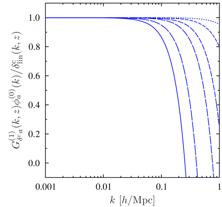
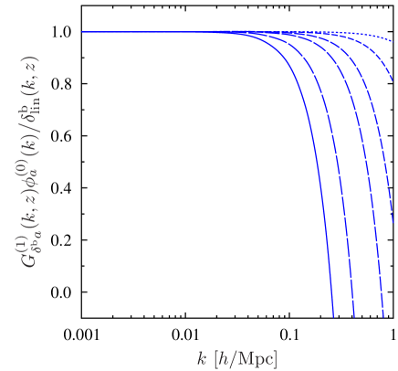
Refer to caption
Refer to caption
Figure 9: Evolution of the initial density perturbations in the CDM plus baryon fluid under the action of the non-linear propagator up to one-loop level, as a function of spatial wavenumber k𝑘k. Left and right panels present results for the CDM and baryon fluctuations, respectively. The linear evolution of the initial perturbation in each species has been scaled out, hence all lines approach unity on large scales. Solid through to dashed lines show results for redshifts z={0,1.0,3.0,5.0,10.0,20.0}𝑧01.03.05.010.020.0z=\{0,1.0,3.0,5.0,10.0,20.0\}.
Refer to caption
Refer to caption
Figure 10: Comparison of the linear and one-loop non-linear power spectrum for the CDM and baryons. Top panels: the absolute power as function of wavenumber. Left panels, show results for CDM, and right for the baryons. Thin (red) lines represent linear theory, and thick (blue) ones non-linear theory. The solid through to dashed lines show results for redshifts z={0,1.0,3.0,5.0,10.0,20.0}𝑧01.03.05.010.020.0z=\{0,1.0,3.0,5.0,10.0,20.0\}. Lowest solid green line shows the initial power spectrum. Bottom panels: show the ratio of the one-loop non-linear to linear theory power spectrum.

VI.2 Power spectra of CDM and baryons

Fig. 10 presents the results for the linear and non-linear evolution of the power spectra in the 2-component fluid model. The left and right panels show results for the CDM and the baryons, respectively. As expected from our discussion in §II.6 and Fig. 2, we see that the initial CDM power spectrum (zi=100subscript𝑧𝑖100z_{i}=100) is very smooth, whereas that for the baryon distribution is highly oscillatory (green solid lines labeled 𝒫cc(0)subscriptsuperscript𝒫0cc{\mathcal{P}}^{(0)}_{\mathrm{c}\mathrm{c}} and 𝒫bb(0)subscriptsuperscript𝒫0bb{\mathcal{P}}^{(0)}_{\mathrm{b}\mathrm{b}} in the plot). As the two fluids evolve under gravity the power grows, and in linear theory (thin red lines) larger amplitude BAO are induced in the CDM spectrum, whilst those in the baryon distribution are slowly damped.

The figure also shows how these results change when the non-linear evolution of the density fields is turned on. The non-linear power spectra are represented as thick blue lines, and we have included all terms up to one-loop level (c.f. Eq. (120)). At z=0𝑧0z=0 and on very large scales (k<0.02hMpc1𝑘0.02superscriptMpc1k<0.02\,h\,{\rm Mpc}^{-1}), the linear and non-linear calculations appear to agree well (solid lines). However, on smaller scales the agreement begins to breakdown. To investigate this in more detail, we take the ratio of the two spectra, and this is plotted in the lower panels of Fig. 2. From this we clearly see that there is a small suppression of power on scales of the order k0.07hMpc1similar-to𝑘0.07superscriptMpc1k\sim 0.07\,h\,{\rm Mpc}^{-1}, this is known as the pre-virialization feature (Smith et al., 2007). This is followed by a strong non-linear amplification at smaller scales. Interestingly, the relative non-linear boost at z=0𝑧0z=0 appears to possess almost identical structure for both CDM and baryons. If we consider earlier times z>0𝑧0z>0 (in the plots denoted by increasingly dashed line styles), then, besides the non-linear boosts being reduced, we note that the curves still maintain the same relative structure. As we will show in §VII, this can be attributed to the fact that the structure of the leading in η𝜂\eta, one-loop corrections, take the same form for both CDM and baryons.

VI.3 Comparison of the exact 2-component fluid with the approximate 1-component fluid

We now explore how our exact 2-component fluid results differ from those that would have been obtained had we used the 1-component fluid approach, along with the approximate recipe as was described in §I. In order to concentrate solely on the approximations introduced by using the 1-component fluid approach, we slightly modify the procedure for obtaining the initial power spectrum, from that set out in §I:

  1. 1’​.

    Fix the cosmological model, specifying ΩcsubscriptΩc\Omega_{\mathrm{c}} and ΩbsubscriptΩb\Omega_{\mathrm{b}}, and hence fbsuperscript𝑓bf^{\rm b}. Solve for the evolution of all perturbed species using the linearized coupled Einstein–Boltzmann equations. Obtain transfer functions for the CDM and baryons at some large redshift say z=100𝑧100z=100.

  2. 2’​.

    Use these transfer functions to generate the linear power spectrum matrix in the 2-component fluid theory, at the present day: i.e. Pab(k,z=0)gaa(z=0)Ta(k)gbb(z=0)Tb(k)Akn.subscript𝑃𝑎𝑏𝑘𝑧0subscript𝑔𝑎superscript𝑎𝑧0subscript𝑇superscript𝑎𝑘subscript𝑔𝑏superscript𝑏𝑧0subscript𝑇superscript𝑏𝑘𝐴superscript𝑘𝑛P_{ab}(k,z=0)\approx g_{aa^{\prime}}(z=0)T_{a^{\prime}}(k)g_{bb^{\prime}}(z=0)T_{b^{\prime}}(k)Ak^{n}\ . Using this power spectrum matrix, define the present day matter power spectrum as

    Pδ¯δ¯(𝐤,z=0)=(1fb)2Pδcδc(𝐤,z=0)+2(1fb)fbPδcδb(𝐤,z=0)+(fb)2Pδbδb(𝐤,z=0).subscript𝑃¯𝛿¯𝛿𝐤𝑧0superscript1superscript𝑓b2subscript𝑃superscript𝛿csuperscript𝛿c𝐤𝑧021superscript𝑓bsuperscript𝑓bsubscript𝑃superscript𝛿csuperscript𝛿b𝐤𝑧0superscriptsuperscript𝑓b2subscript𝑃superscript𝛿bsuperscript𝛿b𝐤𝑧0P_{\bar{\delta}\bar{\delta}}({\bf k},z=0)=(1-f^{\rm b})^{2}P_{{\delta^{\mathrm{c}}}{\delta^{\mathrm{c}}}}({\bf k},z=0)+2(1-f^{\rm b})f^{\rm b}P_{{\delta^{\mathrm{c}}}{\delta^{\mathrm{b}}}}({\bf k},z=0)+(f^{\rm b})^{2}P_{{\delta^{\mathrm{b}}}{\delta^{\mathrm{b}}}}({\bf k},z=0)\,. (133)

    One could further make the approximation that at the present day δ¯=(1fb)δc+fbδbδc¯𝛿1subscript𝑓bsuperscript𝛿csubscript𝑓bsuperscript𝛿bsuperscript𝛿c\bar{\delta}=(1-f_{\mathrm{b}}){\delta^{\mathrm{c}}}+f_{\mathrm{b}}{\delta^{\mathrm{b}}}\approx{\delta^{\mathrm{c}}}, hence approximating the matter power spectrum as

    Pδ¯Aδ¯A(𝐤,z=0)Pδcδc(𝐤,z=0).subscript𝑃subscript¯𝛿Asubscript¯𝛿A𝐤𝑧0subscript𝑃superscript𝛿csuperscript𝛿c𝐤𝑧0P_{\bar{\delta}_{\mathrm{A}}\bar{\delta}_{\mathrm{A}}}({\bf k},z=0)\approx P_{{\delta^{\mathrm{c}}}{\delta^{\mathrm{c}}}}({\bf k},z=0)\,. (134)

There rest of the steps are unchanged from those discussed in §I. We shall refer to the initial conditions obtained using Eq. (133) as the “exact”, and those produced using Eq. (134) as the “approximate” 1-component fluid initial conditions, respectively.

Figs 12 and 12, present the ratio of the exact linear and non-linear CDM (Fig. 12) and baryon (Fig. 12) power spectra, with the power spectrum obtained from modeling CDM and baryons as an effective single matter fluid. The left and right panels show results obtained using the exact and approximate initial conditions for the 1-component fluid calculation. In all cases, the non-linear evolution is followed using the the RPT framework, including all terms up to the one-loop level. For the case of CDM, we clearly see that at high redshift the approximation is rather poor, there being significantly more amplitude in the exact N=2𝑁2N=2 model than the effective N=1𝑁1N=1 model. We also note that there are strong BAO features in the ratio, and these increase with increasing redshift. These features are due to the fact that the z=0𝑧0z=0 transfer function is used to model the initial conditions of the N=1𝑁1N=1 matter fluid, and therefore can suppress power and artificially enhance the BAO. At early stages in the evolution, the systematic errors are between 45%similar-toabsent4percent5\sim 4-5\% at z=20𝑧20z=20, and between 23%similar-toabsent2percent3\sim 2-3\% at z=10𝑧10z=10. However, at later times the approximation is much better, and by z=3𝑧3z=3 the errors are <1%absentpercent1<1\%, and by z=0𝑧0z=0 are <0.5%absentpercent0.5<0.5\%.

On the other hand, the case for the baryons is worse. We see that the exact N=2𝑁2N=2 results show less power than the approximate N=1𝑁1N=1 counterpart and that this suppression increases with increasing redshift. Again we notice that there are BAO features in the residual, and the oscillation amplitude is much more significant. At early stages in the evolution the systematic errors are large: at z=20𝑧20z=20 they are 25%similar-toabsentpercent25\sim 25\%, and by z=10𝑧10z=10 are 15%similar-toabsentpercent15\sim 15\%. At later times the approximation is still quite poor: at z=3𝑧3z=3 the errors are of the order 5%similar-toabsentpercent5\sim 5\%, and by z=0𝑧0z=0 are still between 23%similar-toabsent2percent3\sim 2-3\%.

Refer to caption
Refer to caption
Figure 11: Ratio of the CDM power spectrum obtained from the CDM and baryon 2-component fluid model, to the total matter spectrum obtained from the 1-component fluid approximation, as a function of wavenumber. Thin (red) lines show the ratio of power spectra in linear theory, while thick (blue) lines show the ratio of one-loop non-linear power spectra. Left and right panels: show results for the exact and approximate 1-component fluid initial conditions, respectively. Again, the solid through to dashed lines show results for redshifts z={0,1.0,3.0,5.0,10.0,20.0}𝑧01.03.05.010.020.0z=\{0,1.0,3.0,5.0,10.0,20.0\}.
Refer to caption
Refer to caption
Figure 12: Ratio of the baryon power spectrum obtained from the CDM and baryon 2-component fluid model, to the total matter spectrum obtained from the 1-component fluid approximation, as a function of wavenumber. Thin (red) lines show the ratio of power spectra in linear theory, while thick (blue) lines show the ratio of one-loop non-linear power spectra. Left and right panels: show results for the exact and approximate 1-component fluid initial conditions, respectively. Again, the solid through to dashed lines show results for redshifts z={0,1.0,3.0,5.0,10.0,20.0}𝑧01.03.05.010.020.0z=\{0,1.0,3.0,5.0,10.0,20.0\}.

VI.4 Impact on total matter power spectrum

Since some cosmological probes are only sensitive to the total mass distribution, such as weak gravitational lensing, it is interesting to ask, what is the error between the exact N=2𝑁2N=2 and the approximate N=1𝑁1N=1 fluid dynamics, incurred when modeling the total matter power spectrum. Recall that the total matter power spectrum is defined as,

Pδ¯δ¯(𝐤,z)=(1fb)2Pδcδc(𝐤,z)+2(1fb)fbPδcδb(𝐤,z)+(fb)2Pδbδb(𝐤,z).subscript𝑃¯𝛿¯𝛿𝐤𝑧superscript1superscript𝑓b2subscript𝑃superscript𝛿csuperscript𝛿c𝐤𝑧21superscript𝑓bsuperscript𝑓bsubscript𝑃superscript𝛿csuperscript𝛿b𝐤𝑧superscriptsuperscript𝑓b2subscript𝑃superscript𝛿bsuperscript𝛿b𝐤𝑧P_{\bar{\delta}\bar{\delta}}({\bf k},z)=(1-f^{\rm b})^{2}P_{\delta^{\mathrm{c}}\delta^{\mathrm{c}}}({\bf k},z)+2(1-f^{\rm b})f^{\rm b}P_{\delta^{\mathrm{c}}\delta^{\mathrm{b}}}({\bf k},z)+(f^{\rm b})^{2}P_{\delta^{\mathrm{b}}\delta^{\mathrm{b}}}({\bf k},z)\ . (135)

The results obtained by using the exact and approximate initial conditions for the 1-component fluid model are plotted in the left and right panels of Fig. 13 respectively. We see that the single-fluid approximation based on exact initial conditions is excellent, being accurate to <0.03%absentpercent0.03<0.03\% for all times and scales considered. As we will show in §VII, this spectacular success can be attributed to the fact that the leading in η𝜂\eta, one-loop corrections, depend only on the total mass distribution.

Using the approximate initial conditions for the single-fluid calculation still leads to very good agreement with the full 2-component fluid result on large scales k0.2hMpc1similar-to𝑘0.2superscriptMpc1k\sim 0.2\,h\,{\rm Mpc}^{-1}, with <0.5%absentpercent0.5<0.5\% accuracy for all the times considered. On smaller scales the approximation becomes worse, being of order 0.7%similar-toabsentpercent0.7\sim 0.7\% at k1.0hMpc1similar-to𝑘1.0superscriptMpc1k\sim 1.0\,h\,{\rm Mpc}^{-1}. However, this departure is unlikely to be accurate, since we can not trust the PT results on these small scales. This owes to the fact that the missing higher order loop corrections become increasingly more important. Nevertheless, this point is rather academic, since using the exact initial conditions will give better than 1% precision for the non-linear matter power spectrum down to scales of the order k1.0hMpc1similar-to𝑘1.0superscriptMpc1k\sim 1.0\,h\,{\rm Mpc}^{-1}, as required by future weak lensing surveys, such as Euclid.

Finally, we note that one can easily show that the linear mass power spectrum simply scales with the square of the linear growth factor, even in the 2-component fluid theory. Hence, the ratio of the 2-component fluid linear mass power spectrum to the 1-component fluid model is constant in time. Furthermore, this constant is simply unity, if the 1-component fluid model is set up with exact initial conditions.
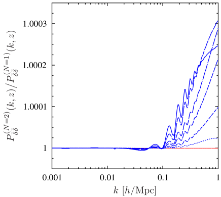
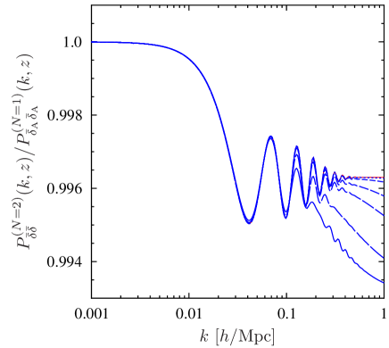
Refer to caption
Refer to caption
Figure 13: Ratio of the total matter power spectrum obtained from the 2-component fluid model for CDM plus baryons, to that obtained from the 1-component fluid approximation, as a function of wavenumber. Again, thin (red) lines show the ratio of power spectra in linear theory, and thick (blue) lines the ratio of one-loop non-linear power spectra. The solid through to dashed lines show results for redshifts z={0,1.0,3.0,5.0,10.0,20.0}𝑧01.03.05.010.020.0z=\{0,1.0,3.0,5.0,10.0,20.0\}. See end of §VI.4 for an explanation as to why the linear theory ratios are independent of time

VII Approximate description of the multi-fluid dynamics

Given that the full expressions for the one-loop corrections to the power spectrum are quite formidable and time consuming to compute, it is of use to attempt to develop an approximate description of these expressions. We present this below. Our approximation scheme is based on insights concerning the late-time behaviour of the one-loop power spectrum, and it is valid for growing mode initial conditions and, although here we present the case of a 2-component fluid, can be generalized for N𝑁N-component matter fluids.

VII.1 Approximate form of the reducible correction

To begin, we recall that the one-loop reducible correction to the power spectrum reads (c.f. Eq. (115))

δPab,R(1)(k,η)=[gac(η)δGbd(1)(k,η)+δGac(1)(k,η)gbd(η)]𝒫cd(0)(k).𝛿subscriptsuperscript𝑃1𝑎𝑏Rk𝜂delimited-[]subscript𝑔𝑎𝑐𝜂𝛿subscriptsuperscript𝐺1𝑏𝑑k𝜂𝛿subscriptsuperscript𝐺1𝑎𝑐k𝜂subscript𝑔𝑏𝑑𝜂subscriptsuperscript𝒫0𝑐𝑑𝑘\delta P^{(1)}_{ab,\mathrm{R}}(\hbox{\bf k},\eta)=\left[g_{ac}(\eta)\delta G^{(1)}_{bd}(\hbox{\bf k},\eta)+\delta G^{(1)}_{ac}(\hbox{\bf k},\eta)g_{bd}(\eta)\right]{\cal P}^{(0)}_{cd}(k)\,. (136)

In the limit of late times, η𝜂\eta\to\infty, we can discard all but the fastest growing modes of the linear propagator, gabsubscript𝑔𝑎𝑏g_{ab}, and one-loop correction to the propagator, δGab(1)𝛿subscriptsuperscript𝐺1𝑎𝑏\delta G^{(1)}_{ab}. For the linear propagator we have simply gab(η)gab,1eηsubscript𝑔𝑎𝑏𝜂subscript𝑔𝑎𝑏1superscripte𝜂g_{ab}(\eta)\to g_{ab,1}{\mathrm{e}}^{\eta}, while for the one-loop correction we find

δGab(1)(k,η)15[3w1f(k)2w1f(k)3w2f(k)2w2f(k)3w1g(k)2w1g(k)3w2g(k)2w2g(k)3w1f(k)2w1f(k)3w2f(k)2w2f(k)3w1g(k)2w1g(k)3w2g(k)2w2g(k)]e3η,𝛿subscriptsuperscript𝐺1𝑎𝑏k𝜂15delimited-[]3subscript𝑤1𝑓𝑘2subscript𝑤1𝑓𝑘3subscript𝑤2𝑓𝑘2subscript𝑤2𝑓𝑘3subscript𝑤1𝑔𝑘2subscript𝑤1𝑔𝑘3subscript𝑤2𝑔𝑘2subscript𝑤2𝑔𝑘3subscript𝑤1𝑓𝑘2subscript𝑤1𝑓𝑘3subscript𝑤2𝑓𝑘2subscript𝑤2𝑓𝑘3subscript𝑤1𝑔𝑘2subscript𝑤1𝑔𝑘3subscript𝑤2𝑔𝑘2subscript𝑤2𝑔𝑘superscripte3𝜂\delta G^{(1)}_{ab}(\hbox{\bf k},\eta)\to\frac{1}{5}\left[\begin{array}[]{cccc}3w_{1}{f(k)}&2w_{1}{f(k)}&3w_{2}{f(k)}&2w_{2}{f(k)}\\ 3w_{1}{g(k)}&2w_{1}{g(k)}&3w_{2}{g(k)}&2w_{2}{g(k)}\\ 3w_{1}{f(k)}&2w_{1}{f(k)}&3w_{2}{f(k)}&2w_{2}{f(k)}\\ 3w_{1}{g(k)}&2w_{1}{g(k)}&3w_{2}{g(k)}&2w_{2}{g(k)}\end{array}\right]{\mathrm{e}}^{3\eta}\,, (137)

where we have

f(k)𝑓𝑘\displaystyle f(k) =\displaystyle= d3k1504k3k15[6k7k179k5k13+50k3k1521kk17+34(k2k12)3(2k2+7k12)ln|kk1|2|k+k1|2]𝒫δ¯δ¯(0)(k1),superscriptd3subscriptk1504superscript𝑘3superscriptsubscript𝑘15delimited-[]6superscript𝑘7subscript𝑘179superscript𝑘5superscriptsubscript𝑘1350superscript𝑘3superscriptsubscript𝑘1521𝑘superscriptsubscript𝑘1734superscriptsuperscript𝑘2superscriptsubscript𝑘1232superscript𝑘27superscriptsubscript𝑘12superscript𝑘subscript𝑘12superscript𝑘subscript𝑘12subscriptsuperscript𝒫0¯𝛿¯𝛿subscript𝑘1\displaystyle\int\frac{{\mathrm{d}}^{3}\hbox{\bf k}_{1}}{504k^{3}k_{1}^{5}}\left[6k^{7}k_{1}-79k^{5}k_{1}^{3}+50k^{3}k_{1}^{5}-21kk_{1}^{7}+\frac{3}{4}(k^{2}-k_{1}^{2})^{3}(2k^{2}+7k_{1}^{2})\ln\frac{|k-k_{1}|^{2}}{|k+k_{1}|^{2}}\right]{\cal P}^{(0)}_{\bar{\delta}\bar{\delta}}(k_{1})\,, (138)
g(k)𝑔𝑘\displaystyle g(k) =\displaystyle= d3k1168k3k15[6k7k141k5k13+2k3k153kk17+34(k2k12)3(2k2+k12)ln|kk1|2|k+k1|2]𝒫δ¯δ¯(0)(k1).superscriptd3subscriptk1168superscript𝑘3superscriptsubscript𝑘15delimited-[]6superscript𝑘7subscript𝑘141superscript𝑘5superscriptsubscript𝑘132superscript𝑘3superscriptsubscript𝑘153𝑘superscriptsubscript𝑘1734superscriptsuperscript𝑘2superscriptsubscript𝑘1232superscript𝑘2superscriptsubscript𝑘12superscript𝑘subscript𝑘12superscript𝑘subscript𝑘12subscriptsuperscript𝒫0¯𝛿¯𝛿subscript𝑘1\displaystyle\int\frac{{\mathrm{d}}^{3}\hbox{\bf k}_{1}}{168k^{3}k_{1}^{5}}\left[6k^{7}k_{1}-41k^{5}k_{1}^{3}+2k^{3}k_{1}^{5}-3kk_{1}^{7}+\frac{3}{4}(k^{2}-k_{1}^{2})^{3}(2k^{2}+k_{1}^{2})\ln\frac{|k-k_{1}|^{2}}{|k+k_{1}|^{2}}\right]{\cal P}^{(0)}_{\bar{\delta}\bar{\delta}}(k_{1})\,\ . (139)

These are just the f𝑓f and g𝑔g functions of (Crocce and Scoccimarro, 2006b), and 𝒫δ¯δ¯(0)(k)subscriptsuperscript𝒫0¯𝛿¯𝛿𝑘{\cal P}^{(0)}_{\bar{\delta}\bar{\delta}}(k) is the initial power spectrum of the total matter fluctuation, δ¯(k)=w1δ1(k)+w2δ2(k)¯𝛿𝑘subscript𝑤1subscript𝛿1𝑘subscript𝑤2subscript𝛿2𝑘\bar{\delta}(k)=w_{1}\delta_{1}(k)+w_{2}\delta_{2}(k):

𝒫δ¯δ¯(0)(k)=w12𝒫11(0)(k)+2w1w2𝒫12(0)(k)+w22𝒫22(0)(k)=[w1T1(k)+w2T2(k)]2𝒫0(k),subscriptsuperscript𝒫0¯𝛿¯𝛿𝑘superscriptsubscript𝑤12subscriptsuperscript𝒫011𝑘2subscript𝑤1subscript𝑤2subscriptsuperscript𝒫012𝑘superscriptsubscript𝑤22subscriptsuperscript𝒫022𝑘superscriptdelimited-[]subscript𝑤1subscript𝑇1𝑘subscript𝑤2subscript𝑇2𝑘2subscript𝒫0𝑘{\cal P}^{(0)}_{\bar{\delta}\bar{\delta}}(k)=w_{1}^{2}{\cal P}^{(0)}_{11}(k)+2w_{1}w_{2}{\cal P}^{(0)}_{12}(k)+w_{2}^{2}{\cal P}^{(0)}_{22}(k)=[w_{1}T_{1}(k)+w_{2}T_{2}(k)]^{2}{\cal P}_{0}(k)\,, (140)

where we have assumed growing mode initial conditions. Upon evaluating Eq. (136) with the approximate form of the propagators as given above, we obtain

δPab,R(1)(k,η)[2f(k)f(k)+g(k)2f(k)f(k)+g(k)f(k)+g(k)2g(k)f(k)+g(k)2g(k)2f(k)f(k)+g(k)2f(k)f(k)+g(k)f(k)+g(k)2g(k)f(k)+g(k)2g(k)]𝒫δ¯δ¯(0)(k)e4η.𝛿subscriptsuperscript𝑃1𝑎𝑏Rk𝜂delimited-[]2𝑓𝑘𝑓𝑘𝑔𝑘2𝑓𝑘𝑓𝑘𝑔𝑘𝑓𝑘𝑔𝑘2𝑔𝑘𝑓𝑘𝑔𝑘2𝑔𝑘2𝑓𝑘𝑓𝑘𝑔𝑘2𝑓𝑘𝑓𝑘𝑔𝑘𝑓𝑘𝑔𝑘2𝑔𝑘𝑓𝑘𝑔𝑘2𝑔𝑘subscriptsuperscript𝒫0¯𝛿¯𝛿𝑘superscripte4𝜂\delta P^{(1)}_{ab,\mathrm{R}}(\hbox{\bf k},\eta)\to\left[\begin{array}[]{cccc}2{f(k)}&{f(k)}+{g(k)}&2{f(k)}&{f(k)}+{g(k)}\\ {f(k)}+{g(k)}&2{g(k)}&{f(k)}+{g(k)}&2{g(k)}\\ 2{f(k)}&{f(k)}+{g(k)}&2{f(k)}&{f(k)}+{g(k)}\\ {f(k)}+{g(k)}&2{g(k)}&{f(k)}+{g(k)}&2{g(k)}\end{array}\right]{\cal P}^{(0)}_{\bar{\delta}\bar{\delta}}(k){\mathrm{e}}^{4\eta}\,. (141)

For early times on the other hand, as η0𝜂0\eta\to 0 we have simply that δPab,R(1)(k,η)0𝛿subscriptsuperscript𝑃1𝑎𝑏Rk𝜂0\delta P^{(1)}_{ab,\mathrm{R}}(\hbox{\bf k},\eta)\to 0. In fact, explicit computation shows that in this limit, the reducible correction vanishes as δPab,R(1)(k,η)(eη1)2\delta P^{(1)}_{ab,\mathrm{R}}(\hbox{\bf k},\eta)\to\propto({\mathrm{e}}^{\eta}-1)^{2}. Since the vanishing of δPab,R(1)(k,η)𝛿subscriptsuperscript𝑃1𝑎𝑏Rk𝜂\delta P^{(1)}_{ab,\mathrm{R}}(\hbox{\bf k},\eta) as η0𝜂0\eta\to 0 is required on physical grounds, we would like to implement it even in the approximate description. To do so, we will simply change the time dependence of Eq. (141) as e4ηe2η(eη1)2superscripte4𝜂superscripte2𝜂superscriptsuperscripte𝜂12{\mathrm{e}}^{4\eta}\to{\mathrm{e}}^{2\eta}({\mathrm{e}}^{\eta}-1)^{2}. Thus we define the approximate one-loop reducible correction to the power spectrum as

δPab,R,A(1)(k,η)[2f(k)f(k)+g(k)2f(k)f(k)+g(k)f(k)+g(k)2g(k)f(k)+g(k)2g(k)2f(k)f(k)+g(k)2f(k)f(k)+g(k)f(k)+g(k)2g(k)f(k)+g(k)2g(k)]𝒫δ¯δ¯(0)(k)e2η(eη1)2.𝛿subscriptsuperscript𝑃1𝑎𝑏RAk𝜂delimited-[]2𝑓𝑘𝑓𝑘𝑔𝑘2𝑓𝑘𝑓𝑘𝑔𝑘𝑓𝑘𝑔𝑘2𝑔𝑘𝑓𝑘𝑔𝑘2𝑔𝑘2𝑓𝑘𝑓𝑘𝑔𝑘2𝑓𝑘𝑓𝑘𝑔𝑘𝑓𝑘𝑔𝑘2𝑔𝑘𝑓𝑘𝑔𝑘2𝑔𝑘subscriptsuperscript𝒫0¯𝛿¯𝛿𝑘superscripte2𝜂superscriptsuperscripte𝜂12\delta P^{(1)}_{ab,\mathrm{R,A}}(\hbox{\bf k},\eta)\equiv\left[\begin{array}[]{cccc}2{f(k)}&{f(k)}+{g(k)}&2{f(k)}&{f(k)}+{g(k)}\\ {f(k)}+{g(k)}&2{g(k)}&{f(k)}+{g(k)}&2{g(k)}\\ 2{f(k)}&{f(k)}+{g(k)}&2{f(k)}&{f(k)}+{g(k)}\\ {f(k)}+{g(k)}&2{g(k)}&{f(k)}+{g(k)}&2{g(k)}\end{array}\right]{\cal P}^{(0)}_{\bar{\delta}\bar{\delta}}(k){\mathrm{e}}^{2\eta}({\mathrm{e}}^{\eta}-1)^{2}\,. (142)

Needless to say, the fastest growing mode is not affected by this substitution.
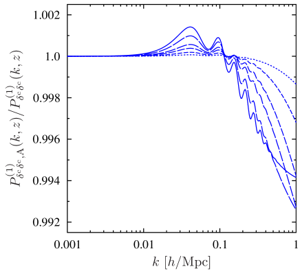
VII.2 Approximate form of the mode-coupling correction

Keeping only the fastest growing mode of the one-loop mode-coupling correction to the power spectrum, we find

δPab,MC(1)(k,η)[2F(k)H(k)2F(k)H(k)H(k)2G(k)H(k)2G(k)2F(k)H(k)2F(k)H(k)H(k)2G(k)H(k)2G(k)]e4η,𝛿subscriptsuperscript𝑃1𝑎𝑏MCk𝜂delimited-[]2𝐹𝑘𝐻𝑘2𝐹𝑘𝐻𝑘𝐻𝑘2𝐺𝑘𝐻𝑘2𝐺𝑘2𝐹𝑘𝐻𝑘2𝐹𝑘𝐻𝑘𝐻𝑘2𝐺𝑘𝐻𝑘2𝐺𝑘superscripte4𝜂\delta P^{(1)}_{ab,\mathrm{MC}}(\hbox{\bf k},\eta)\to\left[\begin{array}[]{cccc}2{F(k)}&{H(k)}&2{F(k)}&{H(k)}\\ {H(k)}&2{G(k)}&{H(k)}&2{G(k)}\\ 2{F(k)}&{H(k)}&2{F(k)}&{H(k)}\\ {H(k)}&2{G(k)}&{H(k)}&2{G(k)}\end{array}\right]{\mathrm{e}}^{4\eta}\,, (143)

where we have defined

F(k)𝐹𝑘\displaystyle F(k) =d3k1k4[7kx+k1(310x2)]2196k12(k22kk1x+k12)2𝒫δ¯δ¯(0)(k1)𝒫δ¯δ¯(0)(k22kk1x+k12),absentsuperscriptd3subscriptk1superscript𝑘4superscriptdelimited-[]7𝑘𝑥subscript𝑘1310superscript𝑥22196superscriptsubscript𝑘12superscriptsuperscript𝑘22𝑘subscript𝑘1𝑥superscriptsubscript𝑘122subscriptsuperscript𝒫0¯𝛿¯𝛿subscript𝑘1subscriptsuperscript𝒫0¯𝛿¯𝛿superscript𝑘22𝑘subscript𝑘1𝑥superscriptsubscript𝑘12\displaystyle=\int{\mathrm{d}}^{3}\hbox{\bf k}_{1}\,\frac{k^{4}\left[7kx+k_{1}\left(3-10x^{2}\right)\right]^{2}}{196k_{1}^{2}\left(k^{2}-2kk_{1}x+k_{1}^{2}\right)^{2}}{\cal P}^{(0)}_{\bar{\delta}\bar{\delta}}(k_{1}){\cal P}^{(0)}_{\bar{\delta}\bar{\delta}}\left(\sqrt{k^{2}-2kk_{1}x+k_{1}^{2}}\right)\,, (144)
G(k)𝐺𝑘\displaystyle G(k) =d3k1k4[7kxk1(1+6x2)]2196k12(k22kk1x+k12)2𝒫δ¯δ¯(0)(k1)𝒫δ¯δ¯(0)(k22kk1x+k12),absentsuperscriptd3subscriptk1superscript𝑘4superscriptdelimited-[]7𝑘𝑥subscript𝑘116superscript𝑥22196superscriptsubscript𝑘12superscriptsuperscript𝑘22𝑘subscript𝑘1𝑥superscriptsubscript𝑘122subscriptsuperscript𝒫0¯𝛿¯𝛿subscript𝑘1subscriptsuperscript𝒫0¯𝛿¯𝛿superscript𝑘22𝑘subscript𝑘1𝑥superscriptsubscript𝑘12\displaystyle=\int{\mathrm{d}}^{3}\hbox{\bf k}_{1}\,\frac{k^{4}\left[7kx-k_{1}(1+6x^{2})\right]^{2}}{196k_{1}^{2}\left(k^{2}-2kk_{1}x+k_{1}^{2}\right)^{2}}{\cal P}^{(0)}_{\bar{\delta}\bar{\delta}}(k_{1}){\cal P}^{(0)}_{\bar{\delta}\bar{\delta}}\left(\sqrt{k^{2}-2kk_{1}x+k_{1}^{2}}\right)\,, (145)
H(k)𝐻𝑘\displaystyle H(k) =d3k1k4[(60x48x23)k1214kk1x(8x21)+49k2x2]98k12(k22kk1x+k12)2𝒫δ¯δ¯(0)(k1)𝒫δ¯δ¯(0)(k22kk1x+k12),absentsuperscriptd3subscriptk1superscript𝑘4delimited-[]60superscript𝑥48superscript𝑥23superscriptsubscript𝑘1214𝑘subscript𝑘1𝑥8superscript𝑥2149superscript𝑘2superscript𝑥298superscriptsubscript𝑘12superscriptsuperscript𝑘22𝑘subscript𝑘1𝑥superscriptsubscript𝑘122subscriptsuperscript𝒫0¯𝛿¯𝛿subscript𝑘1subscriptsuperscript𝒫0¯𝛿¯𝛿superscript𝑘22𝑘subscript𝑘1𝑥superscriptsubscript𝑘12\displaystyle=\int{\mathrm{d}}^{3}\hbox{\bf k}_{1}\,\frac{k^{4}\left[\left(60x^{4}-8x^{2}-3\right)k_{1}^{2}-14kk_{1}x\left(8x^{2}-1\right)+49k^{2}x^{2}\right]}{98k_{1}^{2}\left(k^{2}-2kk_{1}x+k_{1}^{2}\right)^{2}}{\cal P}^{(0)}_{\bar{\delta}\bar{\delta}}(k_{1}){\cal P}^{(0)}_{\bar{\delta}\bar{\delta}}\left(\sqrt{k^{2}-2kk_{1}x+k_{1}^{2}}\right)\,, (146)

where x𝑥x is the cosine of the angle between k and k1subscriptk1\hbox{\bf k}_{1}, i.e. kk1=kk1xksubscriptk1𝑘subscript𝑘1𝑥\hbox{\bf k}\cdot\hbox{\bf k}_{1}=kk_{1}x.

For early times, the situation is completely analogous to the case of the reducible correction: as η0𝜂0\eta\to 0 we have that δPab,MC(1)(k,η)0𝛿subscriptsuperscript𝑃1𝑎𝑏MCk𝜂0\delta P^{(1)}_{ab,\mathrm{MC}}(\hbox{\bf k},\eta)\to 0 and in fact, δPab,MC(1)(k,η)(eη1)2\delta P^{(1)}_{ab,\mathrm{MC}}(\hbox{\bf k},\eta)\to\propto({\mathrm{e}}^{\eta}-1)^{2} in this limit. So again we implement the vanishing of the mode-coupling correction as η0𝜂0\eta\to 0 by simply changing the time dependence of Eq. (143) as e4ηe2η(eη1)2superscripte4𝜂superscripte2𝜂superscriptsuperscripte𝜂12{\mathrm{e}}^{4\eta}\to{\mathrm{e}}^{2\eta}({\mathrm{e}}^{\eta}-1)^{2}. Then the approximate one-loop mode-coupling correction to the power spectrum is defined as

δPab,MC,A(1)(k,η)[2F(k)H(k)2F(k)H(k)H(k)2G(k)H(k)2G(k)2F(k)H(k)2F(k)H(k)H(k)2G(k)H(k)2G(k)]e2η(eη1)2.𝛿subscriptsuperscript𝑃1𝑎𝑏MCAk𝜂delimited-[]2𝐹𝑘𝐻𝑘2𝐹𝑘𝐻𝑘𝐻𝑘2𝐺𝑘𝐻𝑘2𝐺𝑘2𝐹𝑘𝐻𝑘2𝐹𝑘𝐻𝑘𝐻𝑘2𝐺𝑘𝐻𝑘2𝐺𝑘superscripte2𝜂superscriptsuperscripte𝜂12\delta P^{(1)}_{ab,\mathrm{MC,A}}(\hbox{\bf k},\eta)\equiv\left[\begin{array}[]{cccc}2{F(k)}&{H(k)}&2{F(k)}&{H(k)}\\ {H(k)}&2{G(k)}&{H(k)}&2{G(k)}\\ 2{F(k)}&{H(k)}&2{F(k)}&{H(k)}\\ {H(k)}&2{G(k)}&{H(k)}&2{G(k)}\end{array}\right]{\mathrm{e}}^{2\eta}({\mathrm{e}}^{\eta}-1)^{2}\,. (147)

Clearly the fastest growing mode is not affected by this substitution.
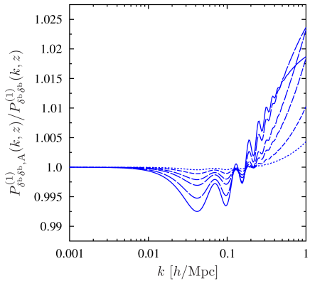
Refer to caption
Refer to caption
Figure 14: Ratio of the approximate to exact one-loop non-linear matter power spectra for CDM (left panel) and baryons (right panel) in the 2-component fluid model for CDM plus baryons. As before, the solid through to dashed lines show results for redshifts z={0, 1.0, 3.0, 5.0, 10.0, 20.0}𝑧01.03.05.010.020.0z=\{0,\,1.0,\,3.0,\,5.0,\,10.0,\,20.0\}. Approximations are good to better than 1% up to k0.2hMpc1𝑘0.2superscriptMpc1k\approx 0.2\,h\,{\rm Mpc}^{-1}.

VII.3 Comparison of the approximate and exact 2-component fluid models

Fig. 14 shows the ratio of the approximate non-linear CDM (left panel) and baryon (right panel) power spectra with the exact 2-component fluid non-linear power spectra:

Pab,A(1)(k,z)Pab(1)(k,z)Pab(0)(k,z)+δPab,R,A(1)+δPab,MC,A(1)(k,z)Pab(0)(k,z)+δPab,R(1)+δPab,MC(1)(k,z),subscriptsuperscript𝑃1𝑎𝑏A𝑘𝑧subscriptsuperscript𝑃1𝑎𝑏𝑘𝑧subscriptsuperscript𝑃0𝑎𝑏𝑘𝑧𝛿subscriptsuperscript𝑃1𝑎𝑏RA𝛿subscriptsuperscript𝑃1𝑎𝑏MCA𝑘𝑧subscriptsuperscript𝑃0𝑎𝑏𝑘𝑧𝛿subscriptsuperscript𝑃1𝑎𝑏R𝛿subscriptsuperscript𝑃1𝑎𝑏MC𝑘𝑧\frac{P^{(1)}_{ab,\mathrm{A}}(k,z)}{P^{(1)}_{ab}(k,z)}\equiv\frac{P^{(0)}_{ab}(k,z)+\delta P^{(1)}_{ab,\mathrm{R,A}}+\delta P^{(1)}_{ab,\mathrm{MC,A}}(k,z)}{P^{(0)}_{ab}(k,z)+\delta P^{(1)}_{ab,\mathrm{R}}+\delta P^{(1)}_{ab,\mathrm{MC}}(k,z)}\,, (148)

where the first term in the numerator is given by Eq. (113) with gabsubscript𝑔𝑎𝑏g_{ab} being the full linear propagator. For the case of CDM, the agreement is very good, being <0.2%absentpercent0.2<0.2\% for k<0.2hMpc1𝑘0.2superscriptMpc1k<0.2\,h\,{\rm Mpc}^{-1} (i.e. on scales large enough for one-loop PT to be trusted), and for all times considered. The approximation performs worse for baryons, however, the agreement is still quite good, being <0.7%absentpercent0.7<0.7\%, on scales of up to k0.2hMpc1similar-to𝑘0.2superscriptMpc1k\sim 0.2\,h\,{\rm Mpc}^{-1}, again for all considered times.

We note in passing that the success of the approximation – which was based on the late time behaviour of the one-loop correction – for relatively early times (say z=10𝑧10z=10202020) is simply a consequence of the fact that at early times the one-loop correction to the power spectrum is small. Hence, even if the approximation of the one-loop correction itself is not very accurate at such times, this does not influence the fact that the full non-linear power spectrum is still well approximated. Clearly, if all of the δP(1)𝛿superscript𝑃1\delta P^{(1)}s are small compared to P(0)superscript𝑃0P^{(0)} in Eq. (148), then the ratio is close to one, irrespective of whether the individual approximations δP(1)δPA(1)𝛿superscript𝑃1𝛿subscriptsuperscript𝑃1A\delta P^{(1)}\approx\delta P^{(1)}_{\mathrm{A}} are particularly good or not.

We thus conclude that the one-loop corrections to the power spectrum for both CDM and baryons are very well-modeled by the leading late time terms, for all scales and times considered. Incidentally, this observation explains two phenomena we encountered earlier. Firstly, as noted in §VI.2, the structure of the non-linear to linear power spectra for the CDM and baryons (see bottom panels of Fig. 10) are almost identical. This is because the leading late time corrections in Eqs (142) and (147) for both CDM and baryons are seen to take precisely the same form. Secondly, the spectacular success of the single-fluid approximation in modeling the total mass power spectrum, noted in §VI.4 (see Fig. 13), is due to the fact the leading late time terms depend only on the average initial field, and not on the two fields separately. Thus, treating the total 2-component fluid as an effective 1-component fluid is exact at the level of the leading non-linear corrections.

Finally, this approximate theory is of great practical advantage, since it reduces the number of numerical integrals to be evaluated by roughly a factor of 10 for the case of the 2-component fluid, so giving an order of magnitude speed up in computational time. Further, the approximate theory can be represented by a compact set of equations.

VIII Summary and Conclusions

In this paper we have generalized the matrix based RPT formalism of Crocce and Scoccimarro (2006a) to the problem of dealing with N𝑁N-component fluids, each of which evolves from a distinct set of initial conditions and contributes to the matter-density and velocity fields.

In §II we showed that, for N𝑁N-component fluids, the essential structure of the RPT framework remained the same as for the N=1𝑁1N=1 case – that is, the equations of motion could be solved in exactly the same way. However, the details of the building blocks of the theory did change: i.e. the vertex, propagator and initial conditions. For N=2𝑁2N=2 the vertex matrix offered no surprises. The linear propagator was more interesting, and we showed that besides the usual growing and decaying modes {D+eη,D(1)e3η/2}formulae-sequenceproportional-tosubscript𝐷superscripte𝜂proportional-tosubscriptsuperscript𝐷1superscripte3𝜂2\{D_{+}\propto{\mathrm{e}}^{\eta},D^{(1)}_{-}\propto{\mathrm{e}}^{-3\eta/2}\}, there were two additional eigenvalues: a static and decaying mode {Dstatconst,D(2)eη/2}formulae-sequenceproportional-tosubscript𝐷statconstproportional-tosubscriptsuperscript𝐷2superscripte𝜂2\{D_{\rm stat}\propto{\rm const},D^{(2)}_{-}\propto{\mathrm{e}}^{-\eta/2}\}. Interestingly, in going to N>2𝑁2N>2 no further time dependence was gained. Unlike the 1-component fluid case, it was no longer possible to choose pure growing modes, unless all of the fluids evolved from identical initial conditions. However, we showed that one can still set up the initial conditions to possess pure large-scale growing modes. All our results were obtained for this specific choice of initial conditions.

In §III it was shown that the equations of motion for the N𝑁N-component fluid case could be solved using a power series solution and that the solutions could be recovered order by order. A graphical representation of the solutions was also described.

In §IV we discussed the statistics of the fields: in particular the covariance matrix of the N𝑁N-component fluid perturbations, and the fully non-linear propagator. This latter quantity can be understood to be the statistic that provides information on the memory of the evolved field to the initial conditions. It also possesses a perturbative expansion and we gave expressions up to one-loop order. A diagrammatic representation was also discussed.

As for the case of the 1-component fluid RPT, we then showed that for the N𝑁N-component fluid RPT the full non-linear power spectrum also possessed a series expansion, and that the series could be grouped into two sub-series, “reducible” and “mode-coupling”. It was shown that the reducible terms were proportional to the initial power spectrum and non-linear propagators. Again we gave complete details for the series up to the one-loop level in the expansions. A diagrammatic description was also discussed.

In §V we developed further the one-loop expressions for the propagator and the mode-coupling contribution to the power spectrum. These expressions were then given for the explicit case of a 2-component fluid.

In §VI we applied the formalism to the problem of modeling the non-linear evolution of a CDM and baryon fluid in the ΛΛ\LambdaCDM paradigm. This enabled us to test the validity of the approximation of treating CDM and baryons as an effective 1-component fluid evolving from a single set of initial conditions, as is currently standard practice.

For the case of CDM, it was shown that the approximation was very good for z<3𝑧3z<3, with the exact and approximate CDM power spectra differing by <1%absentpercent1<1\%. However, for higher redshifts the approximation became progressively worse, it being of the order 3%similar-toabsentpercent3\sim 3\% at z=10𝑧10z=10, with the power in the exact theory being amplified and having weaker BAO features than the approximate theory.

For the case of baryons the situation was worse: at z=20𝑧20z=20 the exact and approximate spectra differed by 25%similar-toabsentpercent25\sim 25\%, and at z=10𝑧10z=10 by 15%similar-toabsentpercent15\sim 15\%. At later times the approximation was still quite poor, and at z=3𝑧3z=3 the errors were of the order 5%similar-toabsentpercent5\sim 5\%, and by z=0𝑧0z=0 were still between 23%similar-toabsent2percent3\sim 2-3\%. The power in the exact theory was suppressed in amplitude but possessed stronger BAO than the corresponding power for the approximate theory.

These conclusions remained essentially unaffected, when the so-called approximate 1-component fluid initial conditions were employed for the effective 1-component fluid computation.

Lastly, we computed the total non-linear matter power spectrum and found that the exact and approximate theory agreed to within <0.03%absentpercent0.03<0.03\%, when the so-called exact 1-component fluid initial conditions were used. Employing the approximate 1-component fluid initial conditions on the other hand leads to an agreement to within <0.5%absentpercent0.5<0.5\% on scales where the perturbation theory was valid k<0.2hMpc1𝑘0.2superscriptMpc1k<0.2\,h\,{\rm Mpc}^{-1} and for all times of interest. Deviations on the order of 0.7%similar-toabsentpercent0.7\sim 0.7\% were found on smaller scales with this approximation.

Our main conclusions therefore are:

  • For theoretical modeling of the low-redshift CDM distribution, the approximate 1-component fluid treatment provides a good approximation. For higher redshift studies, such as those that probe the epoch of reionization, or attempt to model the first objects that form (stars/haloes), then one must be careful to use the appropriate CDM transfer function for the redshift of interest. Otherwise, systematic errors will be present at the level of several percent.

  • For theoretical modeling of baryons in the Universe, a 1-component fluid treatment leads to significant >1%absentpercent1>1\% errors at all times. This implies that cosmological probes that are primarily sensitive to the distributions of baryons in the universe, such as: 21 cm radiation from neutral hydrogen, or the Lyman alpha forest absorption lines in high redshift quasars, can not be modeled using dark matter only simulations at high precision. Instead the baryons must be modeled using a 2-component fluid system of CDM and baryons, with the initial distributions being specified by the linear Einstein–Boltzmann solutions. The correct treatment of CDM and baryon initial conditions may also affect how galaxies form.

  • Observational probes for cosmology that are sensitive to the total mass distribution, such as weak gravitational lensing, can be accurately interpreted using an effective single CDM plus baryon fluid. Thus current modeling technology is good enough for high precision work, but it is highly desirable to use the exact prescription when specifying the initial conditions for the effective single fluid.

Acknowledgments

We thank Ravi Sheth and Patrick McDonald for comments on the text. We acknowledge Martin Crocce, Zhaoming Ma, Roman Scoccimarro and Romain Teyssier for useful discussions. GS acknowledges support from the Hungarian Scientific Research Fund grant OKTA K-60432 and the Swiss National Science Foundation under contract 200020-117602. RES acknowledges support from a Marie Curie Reintegration Grant and partial support from the Swiss National Foundation under contract 200021-116696/1 and WCU grant R32-2008-000-10130-0.

References

  • Crocce and Scoccimarro (2006a) M. Crocce and R. Scoccimarro, PRD 73, 063519 (2006a), eprint arXiv:astro-ph/0509418.
  • Peebles and Ratra (2003) P. J. Peebles and B. Ratra, Reviews of Modern Physics 75, 559 (2003), eprint arXiv:astro-ph/0207347.
  • Spergel et al. (2007) D. N. Spergel, R. Bean, O. Doré, M. R. Nolta, C. L. Bennett, J. Dunkley, G. Hinshaw, N. Jarosik, E. Komatsu, L. Page, et al., ApJS 170, 377 (2007), eprint arXiv:astro-ph/0603449.
  • Komatsu et al. (2009) E. Komatsu, J. Dunkley, M. R. Nolta, C. L. Bennett, B. Gold, G. Hinshaw, N. Jarosik, D. Larson, M. Limon, L. Page, et al., ApJS 180, 330 (2009), eprint 0803.0547.
  • Ma and Bertschinger (1995) C.-P. Ma and E. Bertschinger, ApJ 455, 7 (1995), eprint arXiv:astro-ph/9506072.
  • Seljak and Zaldarriaga (1996) U. Seljak and M. Zaldarriaga, ApJ 469, 437 (1996), eprint arXiv:astro-ph/9603033.
  • Bernardeau et al. (2002) F. Bernardeau, S. Colombi, E. Gaztañaga, and R. Scoccimarro, Phys.  Rep.  367, 1 (2002), eprint arXiv:astro-ph/0112551.
  • Bertschinger (2001) E. Bertschinger, ApJS 137, 1 (2001), eprint arXiv:astro-ph/0103301.
  • Efstathiou et al. (1985) G. Efstathiou, M. Davis, S. D. M. White, and C. S. Frenk, ApJS 57, 241 (1985).
  • Thomas and Couchman (1992) P. A. Thomas and H. M. P. Couchman, MNRAS 257, 11 (1992).
  • Couchman et al. (1995) H. M. P. Couchman, P. A. Thomas, and F. R. Pearce, ApJ 452, 797 (1995), eprint arXiv:astro-ph/9409058.
  • Sugiyama (1995) N. Sugiyama, ApJS 100, 281 (1995), eprint arXiv:astro-ph/9412025.
  • Eisenstein and Hu (1998) D. J. Eisenstein and W. Hu, ApJ 496, 605 (1998), eprint arXiv:astro-ph/9709112.
  • Meiksin et al. (1999) A. Meiksin, M. White, and J. A. Peacock, MNRAS 304, 851 (1999), eprint arXiv:astro-ph/9812214.
  • Pearce et al. (2001) F. R. Pearce, A. Jenkins, C. S. Frenk, S. D. M. White, P. A. Thomas, H. M. P. Couchman, J. A. Peacock, and G. Efstathiou, MNRAS 326, 649 (2001), eprint arXiv:astro-ph/0010587.
  • Teyssier (2002) R. Teyssier, A&A 385, 337 (2002), eprint arXiv:astro-ph/0111367.
  • Springel (2005) V. Springel, MNRAS 364, 1105 (2005), eprint arXiv:astro-ph/0505010.
  • Springel (2009) V. Springel, ArXiv e-prints (2009), eprint 0901.4107.
  • Albrecht et al. (2006) A. Albrecht, G. Bernstein, R. Cahn, W. L. Freedman, J. Hewitt, W. Hu, J. Huth, M. Kamionkowski, E. W. Kolb, L. Knox, et al., ArXiv Astrophysics e-prints (2006), eprint arXiv:astro-ph/0609591.
  • Peacock et al. (2006) J. A. Peacock, P. Schneider, G. Efstathiou, J. R. Ellis, B. Leibundgut, S. J. Lilly, and Y. Mellier, Tech. Rep. (2006).
  • Zhang et al. (2004) P. Zhang, U.-L. Pen, and H. Trac, MNRAS 355, 451 (2004), eprint arXiv:astro-ph/0402115.
  • Iliev et al. (2006) I. T. Iliev, G. Mellema, U.-L. Pen, H. Merz, P. R. Shapiro, and M. A. Alvarez, MNRAS 369, 1625 (2006), eprint arXiv:astro-ph/0512187.
  • Furlanetto et al. (2006) S. R. Furlanetto, S. P. Oh, and F. H. Briggs, Phys.  Rep.  433, 181 (2006), eprint arXiv:astro-ph/0608032.
  • Pillepich et al. (2007) A. Pillepich, C. Porciani, and S. Matarrese, ApJ 662, 1 (2007), eprint arXiv:astro-ph/0611126.
  • Croft et al. (1998) R. A. C. Croft, D. H. Weinberg, N. Katz, and L. Hernquist, ApJ 495, 44 (1998), eprint arXiv:astro-ph/9708018.
  • McDonald et al. (2006) P. McDonald, U. Seljak, S. Burles, D. J. Schlegel, D. H. Weinberg, R. Cen, D. Shih, J. Schaye, D. P. Schneider, N. A. Bahcall, et al., ApJS 163, 80 (2006), eprint arXiv:astro-ph/0405013.
  • Crocce and Scoccimarro (2006b) M. Crocce and R. Scoccimarro, PRD 73, 063520 (2006b), eprint arXiv:astro-ph/0509419.
  • Crocce and Scoccimarro (2008) M. Crocce and R. Scoccimarro, PRD 77, 023533 (2008), eprint arXiv:0704.2783.
  • Nusser (2000) A. Nusser, MNRAS 317, 902 (2000), eprint arXiv:astro-ph/0002317.
  • Matarrese and Mohayaee (2002) S. Matarrese and R. Mohayaee, MNRAS 329, 37 (2002), eprint arXiv:astro-ph/0102220.
  • Shoji and Komatsu (2009) M. Shoji and E. Komatsu, ApJ 700, 705 (2009), eprint 0903.2669.
  • Matarrese and Pietroni (2007) S. Matarrese and M. Pietroni, Journal of Cosmology and Astro-Particle Physics 6, 26 (2007), eprint arXiv:astro-ph/0703563.
  • Matarrese and Pietroni (2008) S. Matarrese and M. Pietroni, Modern Physics Letters A 23, 25 (2008), eprint arXiv:astro-ph/0702653.
  • Bernardeau et al. (2008) F. Bernardeau, M. Crocce, and R. Scoccimarro, PRD 78, 103521 (2008), eprint 0806.2334.
  • Pietroni (2008) M. Pietroni, Journal of Cosmology and Astro-Particle Physics 10, 36 (2008), eprint 0806.0971.
  • Matsubara (2008) T. Matsubara, PRD 78, 083519 (2008), eprint 0807.1733.
  • Wong (2008) Y. Y. Y. Wong, Journal of Cosmology and Astro-Particle Physics 10, 35 (2008), eprint 0809.0693.
  • Saito et al. (2008) S. Saito, M. Takada, and A. Taruya, Physical Review Letters 100, 191301 (2008), eprint 0801.0607.
  • Ichiki et al. (2009) K. Ichiki, M. Takada, and T. Takahashi, PRD 79, 023520 (2009), eprint 0810.4921.
  • Brandbyge et al. (2008) J. Brandbyge, S. Hannestad, T. Haugbølle, and B. Thomsen, Journal of Cosmology and Astro-Particle Physics 8, 20 (2008), eprint 0802.3700.
  • Brandbyge and Hannestad (2009a) J. Brandbyge and S. Hannestad, Journal of Cosmology and Astro-Particle Physics 5, 2 (2009a), eprint 0812.3149.
  • Brandbyge and Hannestad (2009b) J. Brandbyge and S. Hannestad, ArXiv e-prints (2009b), eprint 0908.1969.
  • Lesgourgues et al. (2009) J. Lesgourgues, S. Matarrese, M. Pietroni, and A. Riotto, Journal of Cosmology and Astro-Particle Physics 6, 17 (2009), eprint 0901.4550.
  • Scoccimarro et al. (1998) R. Scoccimarro, S. Colombi, J. N. Fry, J. A. Frieman, E. Hivon, and A. Melott, ApJ 496, 586 (1998), eprint arXiv:astro-ph/9704075.
  • Peebles (1980) P. J. E. Peebles, The large-scale structure of the universe (Research supported by the National Science Foundation. Princeton, N.J., Princeton University Press, 1980. 435 p., 1980).
  • Dodelson (2003) S. Dodelson, Modern cosmology (Modern cosmology / Scott Dodelson. Amsterdam (Netherlands): Academic Press. ISBN 0-12-219141-2, 2003, XIII + 440 p., 2003).
  • Carroll et al. (1992) S. M. Carroll, W. H. Press, and E. L. Turner, Annual Reviews of Astronomy & Astrophysics 30, 499 (1992).
  • Smith et al. (2007) R. E. Smith, R. Scoccimarro, and R. K. Sheth, PRD 75, 063512 (2007), eprint arXiv:astro-ph/0609547.

Appendix A A relation involving the conformal expansion rate

We prove that d/dτ=2[Ωm(a)/2ΩΛ(a)]dd𝜏superscript2delimited-[]subscriptΩm𝑎2subscriptΩΛ𝑎{\mathrm{d}}{\cal H}/{\mathrm{d}}\tau=-{\cal H}^{2}\left[\Omega_{\mathrm{m}}(a)/2-\Omega_{\Lambda}(a)\right]. To begin, we recall that for a homogeneous and isotropic universe, the Einstein field equations reduce to:

3a¨a=4πG(3p+ρ);a˙2+K=8πGρa23,formulae-sequence3¨𝑎𝑎4𝜋𝐺3𝑝𝜌superscript˙𝑎2𝐾8𝜋𝐺𝜌superscript𝑎23\frac{3\ddot{a}}{a}=-4\pi G(3p+\rho)\,;\quad\quad\dot{a}^{2}+K=\frac{8\pi G\rho a^{2}}{3}\,, (149)

where dots denote differentiation with respect to cosmological time t𝑡t. Then for the ΛΛ\LambdaCDM model with matter density ρ=ρm+ρΛ𝜌subscript𝜌𝑚subscript𝜌Λ\rho=\rho_{m}+\rho_{\Lambda} and pressure p=pΛ=ρΛ𝑝subscript𝑝Λsubscript𝜌Λp=p_{\Lambda}=-\rho_{\Lambda}, we find

a¨a=4πGρm3+8πGρΛ3=H2(a)[Ωm(a)2ΩΛ(a)].¨𝑎𝑎4𝜋𝐺subscript𝜌𝑚38𝜋𝐺subscript𝜌Λ3superscript𝐻2𝑎delimited-[]subscriptΩm𝑎2subscriptΩΛ𝑎\frac{\ddot{a}}{a}=-\frac{4\pi G\rho_{m}}{3}+\frac{8\pi G\rho_{\Lambda}}{3}=-H^{2}(a)\left[\frac{\Omega_{\mathrm{m}}(a)}{2}-\Omega_{\Lambda}(a)\right]\,. (150)

Consider now,

ddτ=ddτ(aH)=dtdτddt(a˙)=aa¨.dd𝜏dd𝜏𝑎𝐻d𝑡d𝜏dd𝑡˙𝑎𝑎¨𝑎\frac{{\mathrm{d}}{\cal H}}{{\mathrm{d}}\tau}=\frac{{\mathrm{d}}}{{\mathrm{d}}\tau}(aH)=\frac{{\mathrm{d}}t}{{\mathrm{d}}\tau}\frac{{\mathrm{d}}}{{\mathrm{d}}t}(\dot{a})=a\ddot{a}\,. (151)

The last two equations together give the desired result

ddτ=2[Ωm(a)2ΩΛ(a)].dd𝜏superscript2delimited-[]subscriptΩm𝑎2subscriptΩΛ𝑎\frac{{\mathrm{d}}{\cal H}}{{\mathrm{d}}\tau}=-{\cal H}^{2}\left[\frac{\Omega_{\mathrm{m}}(a)}{2}-\Omega_{\Lambda}(a)\right]\,. (152)

Appendix B Calculating the propagator

B.1 The non-linear propagator

In this appendix we provide explicit details of the calculation of the propagator for the PT solutions up to third order in the expansion for Ψa(n)superscriptsubscriptΨ𝑎𝑛\Psi_{a}^{(n)}. To begin, recall that the propagator is defined through Eq. (104), as

Gab(k,η)δD(kk)δΨa(k,η)[ϕ(0)]δϕb(0)(k).subscript𝐺𝑎𝑏k𝜂superscript𝛿𝐷ksuperscriptkdelimited-⟨⟩𝛿subscriptΨ𝑎k𝜂delimited-[]superscriptitalic-ϕ0𝛿superscriptsubscriptitalic-ϕ𝑏0superscriptkG_{ab}(\hbox{\bf k},\eta)\delta^{D}(\hbox{\bf k}-\hbox{\bf k}^{\prime})\equiv\left<\frac{\delta\Psi_{a}(\hbox{\bf k},\eta)[\phi^{(0)}]}{\delta\phi_{b}^{(0)}(\hbox{\bf k}^{\prime})}\right>\,. (153)

If we insert the series expansion for Ψa(n)subscriptsuperscriptΨ𝑛𝑎\Psi^{(n)}_{a} as given by Eq. (87), then we obtain a series expansion for the propagator.

Gab(k,η)δD(kk)=n=0δΨa(n)(k,η)[ϕ(0)]δϕb(0)(k).subscript𝐺𝑎𝑏k𝜂superscript𝛿𝐷ksuperscriptksubscript𝑛0delimited-⟨⟩𝛿subscriptsuperscriptΨ𝑛𝑎k𝜂delimited-[]superscriptitalic-ϕ0𝛿superscriptsubscriptitalic-ϕ𝑏0superscriptkG_{ab}(\hbox{\bf k},\eta)\delta^{D}(\hbox{\bf k}-\hbox{\bf k}^{\prime})=\sum_{n=0}\left<\frac{\delta\Psi^{(n)}_{a}(\hbox{\bf k},\eta)[\phi^{(0)}]}{\delta\phi_{b}^{(0)}(\hbox{\bf k}^{\prime})}\right>\,. (154)

The next step is to calculate the functional derivatives of the perturbative solutions. Functionals are essentially functions that depend on the full shape of another function over a certain domain. We shall denote functionals using the notation, F[y(x)]𝐹delimited-[]𝑦𝑥F[y(x)], and this has the specific meaning,

F[y(x)]=abdxg(y(x)).𝐹delimited-[]𝑦𝑥superscriptsubscript𝑎𝑏differential-d𝑥𝑔𝑦𝑥F[y(x)]=\int_{a}^{b}{\mathrm{d}}x\,g(y(x))\ . (155)

where g(y)𝑔𝑦g(y) is some arbitrary continuous function. Functional derivatives may be taken using the relation,

dFabdxδFδy(x)|y0(x)δy(x),d𝐹evaluated-atsuperscriptsubscript𝑎𝑏differential-d𝑥𝛿𝐹𝛿𝑦𝑥superscript𝑦0𝑥𝛿𝑦𝑥{\mathrm{d}}F\equiv\int_{a}^{b}{\mathrm{d}}x\left.\frac{\delta F}{\delta y(x)}\right|_{y^{0}(x)}\delta y(x)\ , (156)

where in the above we identify δF/δy(x)|y0(x)evaluated-at𝛿𝐹𝛿𝑦𝑥superscript𝑦0𝑥\left.\delta F/\delta y(x)\right|_{y^{0}(x)} as the functional derivative about the function, y0(x)superscript𝑦0𝑥y^{0}(x).

B.2 Propagator for solutions: n={0,1,2}𝑛012n=\{0,1,2\}

To see how we may use Eq. (156), let us explicitly apply it to the solutions Ψ(n)superscriptΨ𝑛\Psi^{(n)}, for n={0,1,2}𝑛012n=\{0,1,2\}.

  • Solution for n=0𝑛0n=0:

For the linear theory solution we have, Ψa(0)(𝐤,η)=gab(η)ϕb(0)(𝐤).superscriptsubscriptΨ𝑎0𝐤𝜂subscript𝑔𝑎𝑏𝜂superscriptsubscriptitalic-ϕ𝑏0𝐤\Psi_{a}^{(0)}({\bf k},\eta)=g_{ab}(\eta)\phi_{b}^{(0)}({\bf k}). This is not in the form of Eq. (155), but we can easily write it in such a form using the Dirac delta function,

Ψa(0)(𝐤,η)[ϕb(0)(𝐤)]=d3𝐤δD(𝐤𝐤)gab(η)ϕb(0)(𝐤).superscriptsubscriptΨ𝑎0𝐤𝜂delimited-[]superscriptsubscriptitalic-ϕ𝑏0superscript𝐤superscriptd3superscript𝐤superscript𝛿𝐷𝐤superscript𝐤subscript𝑔𝑎𝑏𝜂superscriptsubscriptitalic-ϕ𝑏0superscript𝐤\Psi_{a}^{(0)}({\bf k},\eta)[\phi_{b}^{(0)}({\bf k}^{\prime})]=\int{\mathrm{d}}^{3}{\bf k}^{\prime}\delta^{D}({\bf k}-{\bf k}^{\prime})g_{ab}(\eta)\phi_{b}^{(0)}({\bf k}^{\prime})\ . (157)

Now consider a small change δϕb(0)(𝐤)𝛿subscriptsuperscriptitalic-ϕ0𝑏superscript𝐤\delta\phi^{(0)}_{b}({\bf k}^{\prime}) to the initial conditions ϕb(0)(𝐤)subscriptsuperscriptitalic-ϕ0𝑏superscript𝐤\phi^{(0)}_{b}({\bf k}^{\prime}), whereupon we have

Ψa(0)(𝐤,η)[ϕb(0)(𝐤)+δϕb(0)(𝐤)]superscriptsubscriptΨ𝑎0𝐤𝜂delimited-[]subscriptsuperscriptitalic-ϕ0𝑏superscript𝐤𝛿subscriptsuperscriptitalic-ϕ0𝑏superscript𝐤\displaystyle\Psi_{a}^{(0)}({\bf k},\eta)[\phi^{(0)}_{b}({\bf k}^{\prime})+\delta\phi^{(0)}_{b}({\bf k}^{\prime})] =\displaystyle= d3𝐤δD(𝐤𝐤)gab(η)[ϕb(0)(𝐤)+δϕb(0)(𝐤)]superscriptd3superscript𝐤superscript𝛿𝐷𝐤superscript𝐤subscript𝑔𝑎𝑏𝜂delimited-[]superscriptsubscriptitalic-ϕ𝑏0superscript𝐤𝛿subscriptsuperscriptitalic-ϕ0𝑏superscript𝐤\displaystyle\int{\mathrm{d}}^{3}{\bf k}^{\prime}\delta^{D}({\bf k}-{\bf k}^{\prime})g_{ab}(\eta)\left[\phi_{b}^{(0)}({\bf k}^{\prime})+\delta\phi^{(0)}_{b}({\bf k}^{\prime})\right]\ (158)
=\displaystyle= Ψa(0)(𝐤,η)[ϕb(0)(𝐤)]+d3𝐤δD(𝐤𝐤)gab(η)δϕb(0)(𝐤).superscriptsubscriptΨ𝑎0𝐤𝜂delimited-[]subscriptsuperscriptitalic-ϕ0𝑏superscript𝐤superscriptd3superscript𝐤superscript𝛿𝐷𝐤superscript𝐤subscript𝑔𝑎𝑏𝜂𝛿subscriptsuperscriptitalic-ϕ0𝑏superscript𝐤\displaystyle\Psi_{a}^{(0)}({\bf k},\eta)[\phi^{(0)}_{b}({\bf k}^{\prime})]+\int{\mathrm{d}}^{3}{\bf k}^{\prime}\delta^{D}({\bf k}-{\bf k}^{\prime})g_{ab}(\eta)\delta\phi^{(0)}_{b}({\bf k}^{\prime})\ .

Taking the first term on the right-hand-side over to the left, we find

dΨa(0)(𝐤,η)[ϕb(0)(𝐤)]dsuperscriptsubscriptΨ𝑎0𝐤𝜂delimited-[]subscriptsuperscriptitalic-ϕ0𝑏superscript𝐤\displaystyle{\mathrm{d}}\Psi_{a}^{(0)}({\bf k},\eta)[\phi^{(0)}_{b}({\bf k}^{\prime})] =\displaystyle= d3𝐤δD(𝐤𝐤)gab(η)δϕb(0)(𝐤).superscriptd3superscript𝐤superscript𝛿𝐷𝐤superscript𝐤subscript𝑔𝑎𝑏𝜂𝛿subscriptsuperscriptitalic-ϕ0𝑏superscript𝐤\displaystyle\int{\mathrm{d}}^{3}{\bf k}^{\prime}\delta^{D}({\bf k}-{\bf k}^{\prime})g_{ab}(\eta)\delta\phi^{(0)}_{b}({\bf k}^{\prime})\ . (159)

and on comparing the above with our definition from Eq. (156), we identify the functional derivative as,

δΨa(0)(𝐤,η)δϕb(0)(𝐤)=δD(𝐤𝐤)gab(η).𝛿superscriptsubscriptΨ𝑎0𝐤𝜂𝛿superscriptsubscriptitalic-ϕ𝑏0superscript𝐤superscript𝛿𝐷𝐤superscript𝐤subscript𝑔𝑎𝑏𝜂\frac{\delta\Psi_{a}^{(0)}({\bf k},\eta)}{\delta\phi_{b}^{(0)}({\bf k}^{\prime})}=\delta^{D}({\bf k}-{\bf k}^{\prime})g_{ab}(\eta)\ . (160)

Finally, we are interested in the ensemble average evolution of the mode, and since there are no initial fields remaining there is no stochasticity left in the relation and we simply have,

δΨa(0)(𝐤,η)δϕb(0)(𝐤)=δD(𝐤𝐤)gab(η).delimited-⟨⟩𝛿superscriptsubscriptΨ𝑎0𝐤𝜂𝛿superscriptsubscriptitalic-ϕ𝑏0superscript𝐤superscript𝛿𝐷𝐤superscript𝐤subscript𝑔𝑎𝑏𝜂\left<\frac{\delta\Psi_{a}^{(0)}({\bf k},\eta)}{\delta\phi_{b}^{(0)}({\bf k}^{\prime})}\right>=\delta^{D}({\bf k}-{\bf k}^{\prime})g_{ab}(\eta)\ . (161)
  • Solution for n=1𝑛1n=1:

Let us now turn to the more complicated situation of computing the functional derivatives of the first order solution. The first order solution is a functional of the form,

Ψa(1)(𝐤,η)[ϕc(0)(𝐤1),ϕd(0)(𝐤2)]=0ηdηgab(ηη)d3𝐤1d3𝐤2γbcd(s)(𝐤,𝐤1,𝐤2)gcc(η)ϕc(0)(𝐤1)gdd(η)ϕd(0)(𝐤2).superscriptsubscriptΨ𝑎1𝐤𝜂subscriptsuperscriptitalic-ϕ0superscript𝑐subscript𝐤1subscriptsuperscriptitalic-ϕ0superscript𝑑subscript𝐤2superscriptsubscript0𝜂differential-dsuperscript𝜂subscript𝑔𝑎𝑏𝜂superscript𝜂superscriptd3subscript𝐤1superscriptd3subscript𝐤2subscriptsuperscript𝛾s𝑏𝑐𝑑𝐤subscript𝐤1subscript𝐤2subscript𝑔𝑐superscript𝑐superscript𝜂subscriptsuperscriptitalic-ϕ0superscript𝑐subscript𝐤1subscript𝑔𝑑superscript𝑑superscript𝜂subscriptsuperscriptitalic-ϕ0superscript𝑑subscript𝐤2\Psi_{a}^{(1)}({\bf k},\eta)[\phi^{(0)}_{c^{\prime}}({\bf k}_{1}),\phi^{(0)}_{d^{\prime}}({\bf k}_{2})]=\int_{0}^{\eta}{\mathrm{d}}\eta^{\prime}g_{ab}(\eta-\eta^{\prime})\int{\mathrm{d}}^{3}{\bf k}_{1}{\mathrm{d}}^{3}{\bf k}_{2}\,\gamma^{\mathrm{(s)}}_{bcd}({\bf k},{\bf k}_{1},{\bf k}_{2})g_{cc^{\prime}}(\eta^{\prime})\phi^{(0)}_{c^{\prime}}({\bf k}_{1})g_{dd^{\prime}}(\eta^{\prime})\phi^{(0)}_{d^{\prime}}({\bf k}_{2})\ . (162)

Repeating the procedure of above, we consider a small change δϕa(0)(𝐤)𝛿subscriptsuperscriptitalic-ϕ0superscript𝑎𝐤\delta\phi^{(0)}_{a^{\prime}}({\bf k}) to the initial conditions ϕa(0)(𝐤)subscriptsuperscriptitalic-ϕ0superscript𝑎𝐤\phi^{(0)}_{a^{\prime}}({\bf k}), whereupon we have

dΨa(1)(𝐤,η)[ϕc(0),ϕd(0)]dsuperscriptsubscriptΨ𝑎1𝐤𝜂subscriptsuperscriptitalic-ϕ0superscript𝑐subscriptsuperscriptitalic-ϕ0superscript𝑑\displaystyle{\mathrm{d}}\Psi_{a}^{(1)}({\bf k},\eta)[\phi^{(0)}_{c^{\prime}},\phi^{(0)}_{d^{\prime}}] =\displaystyle= 0ηdηgab(ηη)d3𝐤1d3𝐤2γbcd(s)(𝐤,𝐤1,𝐤2)gcc(η)gdd(η)superscriptsubscript0𝜂differential-dsuperscript𝜂subscript𝑔𝑎𝑏𝜂superscript𝜂superscriptd3subscript𝐤1superscriptd3subscript𝐤2subscriptsuperscript𝛾𝑠𝑏𝑐𝑑𝐤subscript𝐤1subscript𝐤2subscript𝑔𝑐superscript𝑐superscript𝜂subscript𝑔𝑑superscript𝑑superscript𝜂\displaystyle\int_{0}^{\eta}{\mathrm{d}}\eta^{\prime}g_{ab}(\eta-\eta^{\prime})\int{\mathrm{d}}^{3}{\bf k}_{1}{\mathrm{d}}^{3}{\bf k}_{2}\gamma^{(s)}_{bcd}({\bf k},{\bf k}_{1},{\bf k}_{2})g_{cc^{\prime}}(\eta^{\prime})g_{dd^{\prime}}(\eta^{\prime}) (163)
×\displaystyle\times [δϕc(0)(𝐤1)ϕd(0)(𝐤2)+ϕc(0)(𝐤1)δϕd(0)(𝐤2)]delimited-[]𝛿subscriptsuperscriptitalic-ϕ0superscript𝑐subscript𝐤1subscriptsuperscriptitalic-ϕ0superscript𝑑subscript𝐤2subscriptsuperscriptitalic-ϕ0superscript𝑐subscript𝐤1𝛿subscriptsuperscriptitalic-ϕ0superscript𝑑subscript𝐤2\displaystyle\left[\delta\phi^{(0)}_{c^{\prime}}({\bf k}_{1})\phi^{(0)}_{d^{\prime}}({\bf k}_{2})+\phi^{(0)}_{c^{\prime}}({\bf k}_{1})\delta\phi^{(0)}_{d^{\prime}}({\bf k}_{2})\right]\
=\displaystyle= 20ηdηgab(ηη)d3𝐤1d3𝐤2γbcd(s)(𝐤,𝐤1,𝐤2)gcc(η)ϕc(0)(𝐤1)gdd(η)δϕd(0)(𝐤2),2superscriptsubscript0𝜂differential-dsuperscript𝜂subscript𝑔𝑎𝑏𝜂superscript𝜂superscriptd3subscript𝐤1superscriptd3subscript𝐤2subscriptsuperscript𝛾𝑠𝑏𝑐𝑑𝐤subscript𝐤1subscript𝐤2subscript𝑔𝑐superscript𝑐superscript𝜂subscriptsuperscriptitalic-ϕ0superscript𝑐subscript𝐤1subscript𝑔𝑑superscript𝑑superscript𝜂𝛿subscriptsuperscriptitalic-ϕ0superscript𝑑subscript𝐤2\displaystyle 2\int_{0}^{\eta}{\mathrm{d}}\eta^{\prime}g_{ab}(\eta-\eta^{\prime})\int{\mathrm{d}}^{3}{\bf k}_{1}{\mathrm{d}}^{3}{\bf k}_{2}\gamma^{(s)}_{bcd}({\bf k},{\bf k}_{1},{\bf k}_{2})g_{cc^{\prime}}(\eta^{\prime})\phi^{(0)}_{c^{\prime}}({\bf k}_{1})g_{dd^{\prime}}(\eta^{\prime})\delta\phi^{(0)}_{d^{\prime}}({\bf k}_{2})\ ,

where the last equality follows from the fact that owing to the symmetry of the vertex matrix γbcd(s)(𝐤,𝐤1,𝐤2)subscriptsuperscript𝛾𝑠𝑏𝑐𝑑𝐤subscript𝐤1subscript𝐤2\gamma^{(s)}_{bcd}({\bf k},{\bf k}_{1},{\bf k}_{2}), the solutions are symmetric to changes {𝐤1,𝐤2}{𝐤2,𝐤1}subscript𝐤1subscript𝐤2subscript𝐤2subscript𝐤1\{{\bf k}_{1},{\bf k}_{2}\}\rightarrow\{{\bf k}_{2},{\bf k}_{1}\} and {c,d}{d,c}𝑐𝑑𝑑𝑐\{c,d\}\rightarrow\{d,c\}.

We would like to take the functional derivative with respect to the arbitrary initial condition δϕa(0)(𝐤)𝛿subscriptsuperscriptitalic-ϕ0superscript𝑎superscript𝐤\delta\phi^{(0)}_{a^{\prime}}({\bf k}^{\prime}), and so we use the relation

δϕa(0)(𝐤i)=d3𝐤jδD(𝐤i𝐤j)δabKδϕb(0)(𝐤j),𝛿subscriptsuperscriptitalic-ϕ0𝑎subscript𝐤𝑖superscriptd3subscript𝐤𝑗superscript𝛿𝐷subscript𝐤𝑖subscript𝐤𝑗subscriptsuperscript𝛿𝐾𝑎𝑏𝛿subscriptsuperscriptitalic-ϕ0𝑏subscript𝐤𝑗\delta\phi^{(0)}_{a}({\bf k}_{i})=\int{\mathrm{d}}^{3}{\bf k}_{j}\delta^{D}({\bf k}_{i}-{\bf k}_{j})\delta^{K}_{ab}\delta\phi^{(0)}_{b}({\bf k}_{j})\ , (164)

to rewrite the initial conditions in terms of the field that we vary. Hence, Eq. (163), becomes

dΨa(1)(𝐤,η)[ϕc(0)(𝐤1),ϕd(0)(𝐤2)]dsuperscriptsubscriptΨ𝑎1𝐤𝜂subscriptsuperscriptitalic-ϕ0superscript𝑐subscript𝐤1subscriptsuperscriptitalic-ϕ0superscript𝑑subscript𝐤2\displaystyle{\mathrm{d}}\Psi_{a}^{(1)}({\bf k},\eta)[\phi^{(0)}_{c^{\prime}}({\bf k}_{1}),\phi^{(0)}_{d^{\prime}}({\bf k}_{2})] =\displaystyle= 0ηdηgab(ηη)d3𝐤1d3𝐤2γbcd(s)(𝐤,𝐤1,𝐤2)gcc(η)ϕc(0)(𝐤1)gdd(η)superscriptsubscript0𝜂differential-dsuperscript𝜂subscript𝑔𝑎𝑏𝜂superscript𝜂superscriptd3subscript𝐤1superscriptd3subscript𝐤2subscriptsuperscript𝛾𝑠𝑏𝑐𝑑𝐤subscript𝐤1subscript𝐤2subscript𝑔𝑐superscript𝑐superscript𝜂subscriptsuperscriptitalic-ϕ0superscript𝑐subscript𝐤1subscript𝑔𝑑superscript𝑑superscript𝜂\displaystyle\int_{0}^{\eta}{\mathrm{d}}\eta^{\prime}g_{ab}(\eta-\eta^{\prime})\int{\mathrm{d}}^{3}{\bf k}_{1}{\mathrm{d}}^{3}{\bf k}_{2}\gamma^{(s)}_{bcd}({\bf k},{\bf k}_{1},{\bf k}_{2})g_{cc^{\prime}}(\eta^{\prime})\phi^{(0)}_{c^{\prime}}({\bf k}_{1})g_{dd^{\prime}}(\eta^{\prime}) (165)
×\displaystyle\times d3𝐤δD(𝐤1𝐤)δdaKδϕa(0)(𝐤).superscriptd3superscript𝐤superscript𝛿𝐷subscript𝐤1superscript𝐤subscriptsuperscript𝛿𝐾superscript𝑑superscript𝑎𝛿subscriptsuperscriptitalic-ϕ0superscript𝑎superscript𝐤\displaystyle\int{\mathrm{d}}^{3}{\bf k}^{\prime}\delta^{D}({\bf k}_{1}-{\bf k}^{\prime})\delta^{K}_{d^{\prime}a^{\prime}}\delta\phi^{(0)}_{a^{\prime}}({\bf k}^{\prime})\ .

On comparing the above expression with Eq. (156), we identify the functional derivative as

δΨa(1)(𝐤,η)δϕa(0)(𝐤)=δD(𝐤1𝐤)0ηdηgab(ηη)d3𝐤1d3𝐤2γbcd(s)(𝐤,𝐤1,𝐤2)gcc(η)ϕc(0)(𝐤1)gda(η).𝛿superscriptsubscriptΨ𝑎1𝐤𝜂𝛿subscriptsuperscriptitalic-ϕ0superscript𝑎superscript𝐤superscript𝛿𝐷subscript𝐤1superscript𝐤superscriptsubscript0𝜂differential-dsuperscript𝜂subscript𝑔𝑎𝑏𝜂superscript𝜂superscriptd3subscript𝐤1superscriptd3subscript𝐤2subscriptsuperscript𝛾𝑠𝑏𝑐𝑑𝐤subscript𝐤1subscript𝐤2subscript𝑔𝑐superscript𝑐superscript𝜂subscriptsuperscriptitalic-ϕ0superscript𝑐subscript𝐤1subscript𝑔𝑑superscript𝑎superscript𝜂\frac{\delta\Psi_{a}^{(1)}({\bf k},\eta)}{\delta\phi^{(0)}_{a^{\prime}}({\bf k}^{\prime})}=\delta^{D}({\bf k}_{1}-{\bf k}^{\prime})\int_{0}^{\eta}{\mathrm{d}}\eta^{\prime}g_{ab}(\eta-\eta^{\prime})\int{\mathrm{d}}^{3}{\bf k}_{1}{\mathrm{d}}^{3}{\bf k}_{2}\gamma^{(s)}_{bcd}({\bf k},{\bf k}_{1},{\bf k}_{2})g_{cc^{\prime}}(\eta^{\prime})\phi^{(0)}_{c^{\prime}}({\bf k}_{1})g_{da^{\prime}}(\eta^{\prime})\ . (166)

On taking the ensemble average we have ϕc(0)(𝐤1)=0delimited-⟨⟩subscriptsuperscriptitalic-ϕ0superscript𝑐subscript𝐤10\left<\phi^{(0)}_{c^{\prime}}({\bf k}_{1})\right>=0, and hence

δΨa(1)(𝐤,η)δϕa(0)(𝐤)=0.delimited-⟨⟩𝛿superscriptsubscriptΨ𝑎1𝐤𝜂𝛿subscriptsuperscriptitalic-ϕ0superscript𝑎superscript𝐤0\left<\frac{\delta\Psi_{a}^{(1)}({\bf k},\eta)}{\delta\phi^{(0)}_{a^{\prime}}({\bf k}^{\prime})}\right>=0\ . (167)

One direct corollary of this result is that, the propagator for the perturbative solutions which involve an even number of initial conditions is zero. Hence, only odd powers of ϕ(0)superscriptitalic-ϕ0\phi^{(0)} contribute.

  • Solution for n=2𝑛2n=2:

Based on the previous calculation, we expect that the first non-zero contribution to the non-linear propagator is n=2𝑛2n=2, since it involves three initial conditions. This can be computed as follows. The solution is a functional of the form,

Ψa(2)(𝐤,η)[ϕc(0)(𝐤1),ϕf(0)(𝐤3),ϕg(0)(𝐤4)]superscriptsubscriptΨ𝑎2𝐤𝜂subscriptsuperscriptitalic-ϕ0superscript𝑐subscript𝐤1subscriptsuperscriptitalic-ϕ0superscript𝑓subscript𝐤3subscriptsuperscriptitalic-ϕ0superscript𝑔subscript𝐤4\displaystyle\Psi_{a}^{(2)}({\bf k},\eta)[\phi^{(0)}_{c^{\prime}}({\bf k}_{1}),\phi^{(0)}_{f^{\prime}}({\bf k}_{3}),\phi^{(0)}_{g^{\prime}}({\bf k}_{4})] =\displaystyle= 20ηdηgab(ηη)d3𝐤1d3𝐤2γbcd(s)(𝐤,𝐤1,𝐤2)Ψc(0)(𝐤1,η)Ψd(1)(𝐤2,η)2superscriptsubscript0𝜂differential-dsuperscript𝜂subscript𝑔𝑎𝑏𝜂superscript𝜂superscriptd3subscript𝐤1superscriptd3subscript𝐤2subscriptsuperscript𝛾𝑠𝑏𝑐𝑑𝐤subscript𝐤1subscript𝐤2subscriptsuperscriptΨ0𝑐subscript𝐤1superscript𝜂subscriptsuperscriptΨ1𝑑subscript𝐤2superscript𝜂\displaystyle 2\int_{0}^{\eta}{\mathrm{d}}\eta^{\prime}g_{ab}(\eta-\eta^{\prime})\int{\mathrm{d}}^{3}{\bf k}_{1}{\mathrm{d}}^{3}{\bf k}_{2}\gamma^{(s)}_{bcd}({\bf k},{\bf k}_{1},{\bf k}_{2})\Psi^{(0)}_{c}({\bf k}_{1},\eta^{\prime})\Psi^{(1)}_{d}({\bf k}_{2},\eta^{\prime})\ (168)
=\displaystyle= 20ηdηgab(ηη)d3𝐤1d3𝐤2γbcd(s)(𝐤,𝐤1,𝐤2)gcc(η)ϕc(0)(𝐤1)2superscriptsubscript0𝜂differential-dsuperscript𝜂subscript𝑔𝑎𝑏𝜂superscript𝜂superscriptd3subscript𝐤1superscriptd3subscript𝐤2subscriptsuperscript𝛾𝑠𝑏𝑐𝑑𝐤subscript𝐤1subscript𝐤2subscript𝑔𝑐superscript𝑐superscript𝜂subscriptsuperscriptitalic-ϕ0superscript𝑐subscript𝐤1\displaystyle 2\int_{0}^{\eta}{\mathrm{d}}\eta^{\prime}g_{ab}(\eta-\eta^{\prime})\int{\mathrm{d}}^{3}{\bf k}_{1}{\mathrm{d}}^{3}{\bf k}_{2}\gamma^{(s)}_{bcd}({\bf k},{\bf k}_{1},{\bf k}_{2})g_{cc^{\prime}}(\eta^{\prime})\phi^{(0)}_{c^{\prime}}({\bf k}_{1})
×\displaystyle\times 0ηdη′′gde(ηη′′)d3𝐤3d3𝐤4γefg(s)(𝐤2,𝐤3,𝐤4)superscriptsubscript0superscript𝜂differential-dsuperscript𝜂′′subscript𝑔𝑑𝑒superscript𝜂superscript𝜂′′superscriptd3subscript𝐤3superscriptd3subscript𝐤4subscriptsuperscript𝛾𝑠𝑒𝑓𝑔subscript𝐤2subscript𝐤3subscript𝐤4\displaystyle\int_{0}^{\eta^{\prime}}{\mathrm{d}}\eta^{\prime\prime}g_{de}(\eta^{\prime}-\eta^{\prime\prime})\int{\mathrm{d}}^{3}{\bf k}_{3}{\mathrm{d}}^{3}{\bf k}_{4}\gamma^{(s)}_{efg}({\bf k}_{2},{\bf k}_{3},{\bf k}_{4})
×\displaystyle\times gff(η′′)ϕf(0)(𝐤3)ggg(η′′)ϕg(0)(𝐤4),subscript𝑔𝑓superscript𝑓superscript𝜂′′subscriptsuperscriptitalic-ϕ0superscript𝑓subscript𝐤3subscript𝑔𝑔superscript𝑔superscript𝜂′′subscriptsuperscriptitalic-ϕ0superscript𝑔subscript𝐤4\displaystyle g_{ff^{\prime}}(\eta^{\prime\prime})\phi^{(0)}_{f^{\prime}}({\bf k}_{3})g_{gg^{\prime}}(\eta^{\prime\prime})\phi^{(0)}_{g^{\prime}}({\bf k}_{4})\ ,

where the factor of two comes from the fact that the first equation is symmetric to interchanging, {c,d}{d,c}𝑐𝑑𝑑𝑐\{c,d\}\rightarrow\{d,c\} and {𝐤1,𝐤2}{𝐤2,𝐤1}subscript𝐤1subscript𝐤2subscript𝐤2subscript𝐤1\{{\bf k}_{1},{\bf k}_{2}\}\rightarrow\{{\bf k}_{2},{\bf k}_{1}\}. Repeating the procedure of above, we now consider a small change δϕa(0)(𝐤)𝛿subscriptsuperscriptitalic-ϕ0superscript𝑎superscript𝐤\delta\phi^{(0)}_{a^{\prime}}({\bf k}^{\prime}) to the initial conditions ϕa(0)(𝐤)subscriptsuperscriptitalic-ϕ0superscript𝑎superscript𝐤\phi^{(0)}_{a^{\prime}}({\bf k}^{\prime}), whereupon

dΨa(2)(𝐤,η)[ϕc(0)(𝐤1),ϕf(0)(𝐤3),ϕg(0)(𝐤4)]dsuperscriptsubscriptΨ𝑎2𝐤𝜂subscriptsuperscriptitalic-ϕ0superscript𝑐subscript𝐤1subscriptsuperscriptitalic-ϕ0superscript𝑓subscript𝐤3subscriptsuperscriptitalic-ϕ0superscript𝑔subscript𝐤4\displaystyle{\mathrm{d}}\Psi_{a}^{(2)}({\bf k},\eta)[\phi^{(0)}_{c^{\prime}}({\bf k}_{1}),\phi^{(0)}_{f^{\prime}}({\bf k}_{3}),\phi^{(0)}_{g^{\prime}}({\bf k}_{4})] =\displaystyle= 20ηdηgab(ηη)d3𝐤1d3𝐤2γbcd(s)(𝐤,𝐤1,𝐤2)gcc(η)0ηdη′′gde(ηη′′)2superscriptsubscript0𝜂differential-dsuperscript𝜂subscript𝑔𝑎𝑏𝜂superscript𝜂superscriptd3subscript𝐤1superscriptd3subscript𝐤2subscriptsuperscript𝛾𝑠𝑏𝑐𝑑𝐤subscript𝐤1subscript𝐤2subscript𝑔𝑐superscript𝑐superscript𝜂superscriptsubscript0superscript𝜂differential-dsuperscript𝜂′′subscript𝑔𝑑𝑒superscript𝜂superscript𝜂′′\displaystyle 2\int_{0}^{\eta}{\mathrm{d}}\eta^{\prime}g_{ab}(\eta-\eta^{\prime})\int{\mathrm{d}}^{3}{\bf k}_{1}{\mathrm{d}}^{3}{\bf k}_{2}\gamma^{(s)}_{bcd}({\bf k},{\bf k}_{1},{\bf k}_{2})g_{cc^{\prime}}(\eta^{\prime})\int_{0}^{\eta^{\prime}}{\mathrm{d}}\eta^{\prime\prime}g_{de}(\eta^{\prime}-\eta^{\prime\prime}) (169)
×\displaystyle\times d3𝐤3d3𝐤4γefg(s)(𝐤2,𝐤3,𝐤4)gff(η′′)ggg(η′′)[δϕc(0)(𝐤1)ϕf(0)(𝐤3)ϕg(0)(𝐤4)\displaystyle\int{\mathrm{d}}^{3}{\bf k}_{3}{\mathrm{d}}^{3}{\bf k}_{4}\gamma^{(s)}_{efg}({\bf k}_{2},{\bf k}_{3},{\bf k}_{4})g_{ff^{\prime}}(\eta^{\prime\prime})g_{gg^{\prime}}(\eta^{\prime\prime})\left[\delta\phi^{(0)}_{c^{\prime}}({\bf k}_{1})\phi^{(0)}_{f^{\prime}}({\bf k}_{3})\phi^{(0)}_{g^{\prime}}({\bf k}_{4})\right.
+\displaystyle+ ϕc(0)(𝐤1)δϕf(0)(𝐤3)ϕg(0)(𝐤4)+ϕc(0)(𝐤1)ϕf(0)(𝐤3)δϕg(0)(𝐤4)].\displaystyle\left.\phi^{(0)}_{c^{\prime}}({\bf k}_{1})\delta\phi^{(0)}_{f^{\prime}}({\bf k}_{3})\phi^{(0)}_{g^{\prime}}({\bf k}_{4})+\phi^{(0)}_{c^{\prime}}({\bf k}_{1})\phi^{(0)}_{f^{\prime}}({\bf k}_{3})\delta\phi^{(0)}_{g^{\prime}}({\bf k}_{4})\right]\ .

We notice that the last two terms are symmetric to changes {𝐤3,𝐤4}{𝐤4,𝐤3}subscript𝐤3subscript𝐤4subscript𝐤4subscript𝐤3\{{\bf k}_{3},{\bf k}_{4}\}\rightarrow\{{\bf k}_{4},{\bf k}_{3}\} and {f,g}{g,f}𝑓𝑔𝑔𝑓\{f,g\}\rightarrow\{g,f\} and this gives us a factor of 2. Next we use Eq. (164) to repeatedly rewrite the perturbations δϕ(0)𝛿superscriptitalic-ϕ0\delta\phi^{(0)} in terms of the the arbitrary initial field δϕa(0)(𝐤)𝛿subscriptsuperscriptitalic-ϕ0superscript𝑎superscript𝐤\delta\phi^{(0)}_{a^{\prime}}({\bf k}^{\prime}). Hence,

dΨa(2)(𝐤,η)dsuperscriptsubscriptΨ𝑎2𝐤𝜂\displaystyle{\mathrm{d}}\Psi_{a}^{(2)}({\bf k},\eta) =\displaystyle= 20ηdηgab(ηη)d3𝐤1d3𝐤2γbcd(s)(𝐤,𝐤1,𝐤2)gcc(η)0ηdη′′gde(ηη′′)2superscriptsubscript0𝜂differential-dsuperscript𝜂subscript𝑔𝑎𝑏𝜂superscript𝜂superscriptd3subscript𝐤1superscriptd3subscript𝐤2subscriptsuperscript𝛾𝑠𝑏𝑐𝑑𝐤subscript𝐤1subscript𝐤2subscript𝑔𝑐superscript𝑐superscript𝜂superscriptsubscript0superscript𝜂differential-dsuperscript𝜂′′subscript𝑔𝑑𝑒superscript𝜂superscript𝜂′′\displaystyle 2\int_{0}^{\eta}{\mathrm{d}}\eta^{\prime}g_{ab}(\eta-\eta^{\prime})\int{\mathrm{d}}^{3}{\bf k}_{1}{\mathrm{d}}^{3}{\bf k}_{2}\gamma^{(s)}_{bcd}({\bf k},{\bf k}_{1},{\bf k}_{2})g_{cc^{\prime}}(\eta^{\prime})\int_{0}^{\eta^{\prime}}{\mathrm{d}}\eta^{\prime\prime}g_{de}(\eta^{\prime}-\eta^{\prime\prime}) (170)
×\displaystyle\times d3𝐤3d3𝐤4γefg(s)(𝐤2,𝐤3,𝐤4)gff(η′′)ggg(η′′)superscriptd3subscript𝐤3superscriptd3subscript𝐤4subscriptsuperscript𝛾𝑠𝑒𝑓𝑔subscript𝐤2subscript𝐤3subscript𝐤4subscript𝑔𝑓superscript𝑓superscript𝜂′′subscript𝑔𝑔superscript𝑔superscript𝜂′′\displaystyle\int{\mathrm{d}}^{3}{\bf k}_{3}{\mathrm{d}}^{3}{\bf k}_{4}\gamma^{(s)}_{efg}({\bf k}_{2},{\bf k}_{3},{\bf k}_{4})g_{ff^{\prime}}(\eta^{\prime\prime})g_{gg^{\prime}}(\eta^{\prime\prime})
×\displaystyle\times d3𝐤[δD(𝐤1𝐤)δcaKϕf(0)(𝐤3)ϕg(0)(𝐤4)+2ϕc(0)(𝐤1)ϕf(0)(𝐤3)δD(𝐤4𝐤)δgaK]δϕa(0)(𝐤).superscriptd3superscript𝐤delimited-[]superscript𝛿𝐷subscript𝐤1superscript𝐤subscriptsuperscript𝛿𝐾superscript𝑐superscript𝑎subscriptsuperscriptitalic-ϕ0superscript𝑓subscript𝐤3subscriptsuperscriptitalic-ϕ0superscript𝑔subscript𝐤42subscriptsuperscriptitalic-ϕ0superscript𝑐subscript𝐤1subscriptsuperscriptitalic-ϕ0superscript𝑓subscript𝐤3superscript𝛿𝐷subscript𝐤4superscript𝐤subscriptsuperscript𝛿𝐾superscript𝑔superscript𝑎𝛿subscriptsuperscriptitalic-ϕ0superscript𝑎superscript𝐤\displaystyle\int{\mathrm{d}}^{3}{\bf k}^{\prime}\left[\delta^{D}({\bf k}_{1}-{\bf k}^{\prime})\delta^{K}_{c^{\prime}a^{\prime}}\phi^{(0)}_{f^{\prime}}({\bf k}_{3})\phi^{(0)}_{g^{\prime}}({\bf k}_{4})+2\phi^{(0)}_{c^{\prime}}({\bf k}_{1})\phi^{(0)}_{f^{\prime}}({\bf k}_{3})\delta^{D}({\bf k}_{4}-{\bf k}^{\prime})\delta^{K}_{g^{\prime}a^{\prime}}\right]\delta\phi^{(0)}_{a^{\prime}}({\bf k}^{\prime})\ .

On comparing the above with our definition for the functional derivative as given by Eq. (156), we may make the following identification:

δΨa(2)(𝐤,η)δϕa(0)(𝐤)𝛿superscriptsubscriptΨ𝑎2𝐤𝜂𝛿subscriptsuperscriptitalic-ϕ0superscript𝑎superscript𝐤\displaystyle\frac{\delta\Psi_{a}^{(2)}({\bf k},\eta)}{\delta\phi^{(0)}_{a^{\prime}}({\bf k}^{\prime})} =\displaystyle= 20ηdηgab(ηη)d3𝐤1d3𝐤2γbcd(s)(𝐤,𝐤1,𝐤2)gcc(η)0ηdη′′gde(ηη′′)2superscriptsubscript0𝜂differential-dsuperscript𝜂subscript𝑔𝑎𝑏𝜂superscript𝜂superscriptd3subscript𝐤1superscriptd3subscript𝐤2subscriptsuperscript𝛾𝑠𝑏𝑐𝑑𝐤subscript𝐤1subscript𝐤2subscript𝑔𝑐superscript𝑐superscript𝜂superscriptsubscript0superscript𝜂differential-dsuperscript𝜂′′subscript𝑔𝑑𝑒superscript𝜂superscript𝜂′′\displaystyle 2\int_{0}^{\eta}{\mathrm{d}}\eta^{\prime}g_{ab}(\eta-\eta^{\prime})\int{\mathrm{d}}^{3}{\bf k}_{1}{\mathrm{d}}^{3}{\bf k}_{2}\gamma^{(s)}_{bcd}({\bf k},{\bf k}_{1},{\bf k}_{2})g_{cc^{\prime}}(\eta^{\prime})\int_{0}^{\eta^{\prime}}{\mathrm{d}}\eta^{\prime\prime}g_{de}(\eta^{\prime}-\eta^{\prime\prime}) (171)
×\displaystyle\times d3𝐤3d3𝐤4γefg(s)(𝐤2,𝐤3,𝐤4)gff(η′′)ggg(η′′)superscriptd3subscript𝐤3superscriptd3subscript𝐤4subscriptsuperscript𝛾𝑠𝑒𝑓𝑔subscript𝐤2subscript𝐤3subscript𝐤4subscript𝑔𝑓superscript𝑓superscript𝜂′′subscript𝑔𝑔superscript𝑔superscript𝜂′′\displaystyle\int{\mathrm{d}}^{3}{\bf k}_{3}{\mathrm{d}}^{3}{\bf k}_{4}\gamma^{(s)}_{efg}({\bf k}_{2},{\bf k}_{3},{\bf k}_{4})g_{ff^{\prime}}(\eta^{\prime\prime})g_{gg^{\prime}}(\eta^{\prime\prime})
×\displaystyle\times [δD(𝐤1𝐤)δcaKϕf(0)(𝐤3)ϕg(0)(𝐤4)+2ϕc(0)(𝐤1)ϕf(0)(𝐤3)δD(𝐤4𝐤)δgaK].delimited-[]superscript𝛿𝐷subscript𝐤1superscript𝐤subscriptsuperscript𝛿𝐾superscript𝑐superscript𝑎subscriptsuperscriptitalic-ϕ0superscript𝑓subscript𝐤3subscriptsuperscriptitalic-ϕ0superscript𝑔subscript𝐤42subscriptsuperscriptitalic-ϕ0superscript𝑐subscript𝐤1subscriptsuperscriptitalic-ϕ0superscript𝑓subscript𝐤3superscript𝛿𝐷subscript𝐤4superscript𝐤subscriptsuperscript𝛿𝐾superscript𝑔superscript𝑎\displaystyle\left[\delta^{D}({\bf k}_{1}-{\bf k}^{\prime})\delta^{K}_{c^{\prime}a^{\prime}}\phi^{(0)}_{f^{\prime}}({\bf k}_{3})\phi^{(0)}_{g^{\prime}}({\bf k}_{4})+2\phi^{(0)}_{c^{\prime}}({\bf k}_{1})\phi^{(0)}_{f^{\prime}}({\bf k}_{3})\delta^{D}({\bf k}_{4}-{\bf k}^{\prime})\delta^{K}_{g^{\prime}a^{\prime}}\right]\ .

Finally, we take the ensemble average and find that the term in square brackets becomes,

\displaystyle\rightarrow [δD(𝐤1𝐤)δcaKϕf(0)(𝐤3)ϕg(0)(𝐤4)+2ϕc(0)(𝐤1)ϕf(0)(𝐤3)δD(𝐤4𝐤)δgaK];delimited-[]superscript𝛿𝐷subscript𝐤1superscript𝐤subscriptsuperscript𝛿𝐾superscript𝑐superscript𝑎delimited-⟨⟩subscriptsuperscriptitalic-ϕ0superscript𝑓subscript𝐤3subscriptsuperscriptitalic-ϕ0superscript𝑔subscript𝐤42delimited-⟨⟩subscriptsuperscriptitalic-ϕ0superscript𝑐subscript𝐤1subscriptsuperscriptitalic-ϕ0superscript𝑓subscript𝐤3superscript𝛿𝐷subscript𝐤4superscript𝐤subscriptsuperscript𝛿𝐾superscript𝑔superscript𝑎\displaystyle\left[\delta^{D}({\bf k}_{1}-{\bf k}^{\prime})\delta^{K}_{c^{\prime}a^{\prime}}\left<\phi^{(0)}_{f^{\prime}}({\bf k}_{3})\phi^{(0)}_{g^{\prime}}({\bf k}_{4})\right>+2\left<\phi^{(0)}_{c^{\prime}}({\bf k}_{1})\phi^{(0)}_{f^{\prime}}({\bf k}_{3})\right>\delta^{D}({\bf k}_{4}-{\bf k}^{\prime})\delta^{K}_{g^{\prime}a^{\prime}}\right]\ ;
\displaystyle\rightarrow [δD(𝐤1𝐤)δcaK𝒫fg(0)(𝐤3)δD(𝐤3+𝐤4)+2𝒫cf(0)(𝐤1)δD(𝐤1+𝐤3)δD(𝐤4𝐤)δgaK].delimited-[]superscript𝛿𝐷subscript𝐤1superscript𝐤subscriptsuperscript𝛿𝐾superscript𝑐superscript𝑎subscriptsuperscript𝒫0superscript𝑓superscript𝑔subscript𝐤3superscript𝛿𝐷subscript𝐤3subscript𝐤42subscriptsuperscript𝒫0superscript𝑐superscript𝑓subscript𝐤1superscript𝛿𝐷subscript𝐤1subscript𝐤3superscript𝛿𝐷subscript𝐤4superscript𝐤subscriptsuperscript𝛿𝐾superscript𝑔superscript𝑎\displaystyle\left[\delta^{D}({\bf k}_{1}-{\bf k}^{\prime})\delta^{K}_{c^{\prime}a^{\prime}}{\cal P}^{(0)}_{f^{\prime}g^{\prime}}({\bf k}_{3})\delta^{D}({\bf k}_{3}+{\bf k}_{4})+2{\cal P}^{(0)}_{c^{\prime}f^{\prime}}({\bf k}_{1})\delta^{D}({\bf k}_{1}+{\bf k}_{3})\delta^{D}({\bf k}_{4}-{\bf k}^{\prime})\delta^{K}_{g^{\prime}a^{\prime}}\right]\ . (172)

Consider the first term in this bracket, we note that it contains a δD(𝐤3+𝐤4)superscript𝛿𝐷subscript𝐤3subscript𝐤4\delta^{D}({\bf k}_{3}+{\bf k}_{4}). If we integrate this first term over 𝐤4subscript𝐤4{\bf k}_{4} then the resulting expression involves γefg(s)(𝐤2,𝐤3,𝐤3)subscriptsuperscript𝛾𝑠𝑒𝑓𝑔subscript𝐤2subscript𝐤3subscript𝐤3\gamma^{(s)}_{efg}({\bf k}_{2},{\bf k}_{3},-{\bf k}_{3}), which from momentum conservation means that waves with equal and opposite momenta enter the interaction and so completely cancel and no wave exits. Thus, the above expression reduces to

δΨa(2)(𝐤,η)δϕa(0)(𝐤)delimited-⟨⟩𝛿superscriptsubscriptΨ𝑎2𝐤𝜂𝛿subscriptsuperscriptitalic-ϕ0superscript𝑎superscript𝐤\displaystyle\left<\frac{\delta\Psi_{a}^{(2)}({\bf k},\eta)}{\delta\phi^{(0)}_{a^{\prime}}({\bf k}^{\prime})}\right> =\displaystyle= 40ηdηgab(ηη)d3𝐤1d3𝐤2γ¯bcd(s)(𝐤1,𝐤2)δD(𝐤𝐤1𝐤2)gcc(η)0ηdη′′gde(ηη′′)4superscriptsubscript0𝜂differential-dsuperscript𝜂subscript𝑔𝑎𝑏𝜂superscript𝜂superscriptd3subscript𝐤1superscriptd3subscript𝐤2subscriptsuperscript¯𝛾𝑠𝑏𝑐𝑑subscript𝐤1subscript𝐤2superscript𝛿𝐷𝐤subscript𝐤1subscript𝐤2subscript𝑔𝑐superscript𝑐superscript𝜂superscriptsubscript0superscript𝜂differential-dsuperscript𝜂′′subscript𝑔𝑑𝑒superscript𝜂superscript𝜂′′\displaystyle 4\int_{0}^{\eta}{\mathrm{d}}\eta^{\prime}g_{ab}(\eta-\eta^{\prime})\int{\mathrm{d}}^{3}{\bf k}_{1}{\mathrm{d}}^{3}{\bf k}_{2}\bar{\gamma}^{(s)}_{bcd}({\bf k}_{1},{\bf k}_{2})\delta^{D}({\bf k}-{\bf k}_{1}-{\bf k}_{2})g_{cc^{\prime}}(\eta^{\prime})\int_{0}^{\eta^{\prime}}{\mathrm{d}}\eta^{\prime\prime}g_{de}(\eta^{\prime}-\eta^{\prime\prime}) (173)
×d3𝐤3d3𝐤4γ¯efg(s)(𝐤3,𝐤4)δD(𝐤2𝐤3𝐤4)gff(η′′)gga(η′′)𝒫cf(0)(𝐤1)δD(𝐤1+𝐤3)δD(𝐤4𝐤).\displaystyle\times\int{\mathrm{d}}^{3}{\bf k}_{3}{\mathrm{d}}^{3}{\bf k}_{4}\bar{\gamma}^{(s)}_{efg}({\bf k}_{3},{\bf k}_{4})\delta^{D}({\bf k}_{2}-{\bf k}_{3}-{\bf k}_{4})g_{ff^{\prime}}(\eta^{\prime\prime})g_{ga^{\prime}}(\eta^{\prime\prime}){\cal P}^{(0)}_{c^{\prime}f^{\prime}}({\bf k}_{1})\delta^{D}({\bf k}_{1}+{\bf k}_{3})\delta^{D}({\bf k}_{4}-{\bf k}^{\prime})\ .

If we integrate over 𝐤4subscript𝐤4{\bf k}_{4}, then 𝐤3subscript𝐤3{\bf k}_{3}, and finally over 𝐤2subscript𝐤2{\bf k}_{2}, then we obtain the desired expression,

δΨa(2)(𝐤,η)δϕa(0)(𝐤)delimited-⟨⟩𝛿superscriptsubscriptΨ𝑎2𝐤𝜂𝛿subscriptsuperscriptitalic-ϕ0superscript𝑎superscript𝐤\displaystyle\left<\frac{\delta\Psi_{a}^{(2)}({\bf k},\eta)}{\delta\phi^{(0)}_{a^{\prime}}({\bf k}^{\prime})}\right> =\displaystyle= δD(𝐤𝐤)×40ηdηgab(ηη)d3𝐤1γ¯bcd(s)(𝐤1,𝐤𝐤1)gcc(η)0ηdη′′gde(ηη′′)superscript𝛿𝐷𝐤superscript𝐤4superscriptsubscript0𝜂differential-dsuperscript𝜂subscript𝑔𝑎𝑏𝜂superscript𝜂superscriptd3subscript𝐤1subscriptsuperscript¯𝛾𝑠𝑏𝑐𝑑subscript𝐤1𝐤subscript𝐤1subscript𝑔𝑐superscript𝑐superscript𝜂superscriptsubscript0superscript𝜂differential-dsuperscript𝜂′′subscript𝑔𝑑𝑒superscript𝜂superscript𝜂′′\displaystyle\delta^{D}({\bf k}-{\bf k}^{\prime})\times 4\int_{0}^{\eta}{\mathrm{d}}\eta^{\prime}g_{ab}(\eta-\eta^{\prime})\int{\mathrm{d}}^{3}{\bf k}_{1}\bar{\gamma}^{(s)}_{bcd}({\bf k}_{1},{\bf k}-{\bf k}_{1})g_{cc^{\prime}}(\eta^{\prime})\int_{0}^{\eta^{\prime}}{\mathrm{d}}\eta^{\prime\prime}g_{de}(\eta^{\prime}-\eta^{\prime\prime}) (174)
×\displaystyle\times γ¯efg(s)(𝐤1,𝐤)gff(η′′)gga(η′′)𝒫cf(0)(𝐤1).subscriptsuperscript¯𝛾𝑠𝑒𝑓𝑔subscript𝐤1superscript𝐤subscript𝑔𝑓superscript𝑓superscript𝜂′′subscript𝑔𝑔superscript𝑎superscript𝜂′′subscriptsuperscript𝒫0superscript𝑐superscript𝑓subscript𝐤1\displaystyle\bar{\gamma}^{(s)}_{efg}(-{\bf k}_{1},{\bf k}^{\prime})g_{ff^{\prime}}(\eta^{\prime\prime})g_{ga^{\prime}}(\eta^{\prime\prime}){\cal P}^{(0)}_{c^{\prime}f^{\prime}}({\bf k}_{1})\ .

Finally, if we assume large-scale growing mode initial conditions ua=(1,1,,1,1)subscript𝑢𝑎1111u_{a}=(1,1,\dots,1,1), then we find the first non-zero perturbative correction to the propagator is given by:

δGaa(1)(𝐤,η)𝛿subscriptsuperscript𝐺1𝑎superscript𝑎𝐤𝜂\displaystyle\delta G^{(1)}_{aa^{\prime}}({\bf k},\eta) =\displaystyle= 40ηdηgab(ηη)d3𝐤1γ¯bcd(s)(𝐤1,𝐤𝐤1)gcc(η)Tc(k1)0ηdη′′gde(ηη′′)4superscriptsubscript0𝜂differential-dsuperscript𝜂subscript𝑔𝑎𝑏𝜂superscript𝜂superscriptd3subscript𝐤1subscriptsuperscript¯𝛾𝑠𝑏𝑐𝑑subscript𝐤1𝐤subscript𝐤1subscript𝑔𝑐superscript𝑐superscript𝜂subscript𝑇superscript𝑐subscript𝑘1superscriptsubscript0superscript𝜂differential-dsuperscript𝜂′′subscript𝑔𝑑𝑒superscript𝜂superscript𝜂′′\displaystyle 4\int_{0}^{\eta}{\mathrm{d}}\eta^{\prime}g_{ab}(\eta-\eta^{\prime})\int{\mathrm{d}}^{3}{\bf k}_{1}\bar{\gamma}^{(s)}_{bcd}({\bf k}_{1},{\bf k}-{\bf k}_{1})g_{cc^{\prime}}(\eta^{\prime})T_{c^{\prime}}(k_{1})\int_{0}^{\eta^{\prime}}{\mathrm{d}}\eta^{\prime\prime}g_{de}(\eta^{\prime}-\eta^{\prime\prime}) (175)
×\displaystyle\times γ¯efg(s)(𝐤1,𝐤)gff(η′′)Tf(k1)gga(η′′)𝒫0(𝐤1).subscriptsuperscript¯𝛾𝑠𝑒𝑓𝑔subscript𝐤1superscript𝐤subscript𝑔𝑓superscript𝑓superscript𝜂′′subscript𝑇superscript𝑓subscript𝑘1subscript𝑔𝑔superscript𝑎superscript𝜂′′subscript𝒫0subscript𝐤1\displaystyle\bar{\gamma}^{(s)}_{efg}(-{\bf k}_{1},{\bf k}^{\prime})g_{ff^{\prime}}(\eta^{\prime\prime})T_{f^{\prime}}(k_{1})g_{ga^{\prime}}(\eta^{\prime\prime}){\mathcal{P}}_{0}({\bf k}_{1})\ .

Appendix C Calculating the mode-coupling power spectrum

In this appendix, we present details of the computation of the mode-coupling contribution to the one-loop power spectrum given by Eq. (119). In Eq. (114) we identified this term as,

Ψa(1)(𝐤)Ψa(1)(𝐤)delimited-⟨⟩subscriptsuperscriptΨ1𝑎𝐤subscriptsuperscriptΨ1superscript𝑎superscript𝐤\displaystyle\left<\Psi^{(1)}_{a}({\bf k})\Psi^{(1)}_{a^{\prime}}({\bf k}^{\prime})\right> =\displaystyle= 0ηdη1gab(ηη1)d3𝐤1d3𝐤2γbcd(s)(k,k1,k2)gce(η1)gdf(η1)ϕe(0)(k1)ϕf(0)(k2)\displaystyle\Bigg{\langle}\int_{0}^{\eta}{\mathrm{d}}\eta_{1}\,g_{ab}(\eta-\eta_{1})\int{\mathrm{d}}^{3}{\bf k}_{1}\,{\mathrm{d}}^{3}{\bf k}_{2}\,\gamma^{\mathrm{(s)}}_{bcd}(\hbox{\bf k},\hbox{\bf k}_{1},\hbox{\bf k}_{2})g_{ce}(\eta_{1})\,g_{df}(\eta_{1})\,\phi^{(0)}_{e}(\hbox{\bf k}_{1})\phi^{(0)}_{f}(\hbox{\bf k}_{2}) (176)
×\displaystyle\times 0ηdη2gab(ηη2)d3𝐤3d3𝐤4γbcd(s)(k,k3,k4)gce(η2)gdf(η2)ϕe(0)(k3)ϕf(0)(k4)\displaystyle\int_{0}^{\eta}{\mathrm{d}}\eta_{2}\,g_{a^{\prime}b^{\prime}}(\eta-\eta_{2})\int{\mathrm{d}}^{3}{\bf k}_{3}\,{\mathrm{d}}^{3}{\bf k}_{4}\,\gamma^{\mathrm{(s)}}_{b^{\prime}c^{\prime}d^{\prime}}(\hbox{\bf k}^{\prime},\hbox{\bf k}_{3},\hbox{\bf k}_{4})g_{c^{\prime}e^{\prime}}(\eta_{2})\,g_{d^{\prime}f^{\prime}}(\eta_{2})\,\phi^{(0)}_{e^{\prime}}(\hbox{\bf k}_{3})\phi^{(0)}_{f^{\prime}}(\hbox{\bf k}_{4})\Bigg{\rangle}\
=\displaystyle= i=14d3𝐤i0ηdη2gab(ηη2)γbcd(s)(k,k3,k4)gce(η2)gdf(η2)superscriptsubscriptproduct𝑖14superscriptd3subscript𝐤𝑖superscriptsubscript0𝜂differential-dsubscript𝜂2subscript𝑔superscript𝑎superscript𝑏𝜂subscript𝜂2subscriptsuperscript𝛾ssuperscript𝑏superscript𝑐superscript𝑑superscriptksubscriptk3subscriptk4subscript𝑔superscript𝑐superscript𝑒subscript𝜂2subscript𝑔superscript𝑑superscript𝑓subscript𝜂2\displaystyle\int\prod_{i=1}^{4}{\mathrm{d}}^{3}{\bf k}_{i}\int_{0}^{\eta}{\mathrm{d}}\eta_{2}\,g_{a^{\prime}b^{\prime}}(\eta-\eta_{2})\gamma^{\mathrm{(s)}}_{b^{\prime}c^{\prime}d^{\prime}}(\hbox{\bf k}^{\prime},\hbox{\bf k}_{3},\hbox{\bf k}_{4})g_{c^{\prime}e^{\prime}}(\eta_{2})\,g_{d^{\prime}f^{\prime}}(\eta_{2})\,
×\displaystyle\times 0ηdη1gab(ηη1)γbcd(s)(k,k1,k2)gce(η1)gdf(η1)ϕe(0)(k1)ϕf(0)(k2)ϕe(0)(k3)ϕf(0)(k4).superscriptsubscript0𝜂differential-dsubscript𝜂1subscript𝑔𝑎𝑏𝜂subscript𝜂1subscriptsuperscript𝛾s𝑏𝑐𝑑ksubscriptk1subscriptk2subscript𝑔𝑐𝑒subscript𝜂1subscript𝑔𝑑𝑓subscript𝜂1delimited-⟨⟩subscriptsuperscriptitalic-ϕ0𝑒subscriptk1subscriptsuperscriptitalic-ϕ0𝑓subscriptk2subscriptsuperscriptitalic-ϕ0superscript𝑒subscriptk3subscriptsuperscriptitalic-ϕ0superscript𝑓subscriptk4\displaystyle\int_{0}^{\eta}{\mathrm{d}}\eta_{1}\,g_{ab}(\eta-\eta_{1})\gamma^{\mathrm{(s)}}_{bcd}(\hbox{\bf k},\hbox{\bf k}_{1},\hbox{\bf k}_{2})g_{ce}(\eta_{1})\,g_{df}(\eta_{1})\,\left<\phi^{(0)}_{e}(\hbox{\bf k}_{1})\phi^{(0)}_{f}(\hbox{\bf k}_{2})\phi^{(0)}_{e^{\prime}}(\hbox{\bf k}_{3})\phi^{(0)}_{f^{\prime}}(\hbox{\bf k}_{4})\right>\ .

On assuming Gaussian initial conditions we may use Wick’s theorem to rewrite the product of initial fields,

ϕe(0)(k1)ϕf(0)(k2)ϕe(0)(k3)ϕf(0)(k4)delimited-⟨⟩subscriptsuperscriptitalic-ϕ0𝑒subscriptk1subscriptsuperscriptitalic-ϕ0𝑓subscriptk2subscriptsuperscriptitalic-ϕ0superscript𝑒subscriptk3subscriptsuperscriptitalic-ϕ0superscript𝑓subscriptk4\displaystyle\left<\phi^{(0)}_{e}(\hbox{\bf k}_{1})\phi^{(0)}_{f}(\hbox{\bf k}_{2})\phi^{(0)}_{e^{\prime}}(\hbox{\bf k}_{3})\phi^{(0)}_{f^{\prime}}(\hbox{\bf k}_{4})\right> =\displaystyle= [𝒫ef(𝐤1)δD(𝐤1+𝐤2)𝒫ef(𝐤3)δD(𝐤3+𝐤4)\displaystyle\left[{\mathcal{P}}_{ef}({\bf k}_{1})\delta^{D}({\bf k}_{1}+{\bf k}_{2}){\mathcal{P}}_{e^{\prime}f^{\prime}}({\bf k}_{3})\delta^{D}({\bf k}_{3}+{\bf k}_{4})\right. (177)
+\displaystyle+ 𝒫ee(𝐤1)δD(𝐤1+𝐤3)𝒫ff(𝐤2)δD(𝐤2+𝐤4)subscript𝒫𝑒superscript𝑒subscript𝐤1superscript𝛿𝐷subscript𝐤1subscript𝐤3subscript𝒫𝑓superscript𝑓subscript𝐤2superscript𝛿𝐷subscript𝐤2subscript𝐤4\displaystyle{\mathcal{P}}_{ee^{\prime}}({\bf k}_{1})\delta^{D}({\bf k}_{1}+{\bf k}_{3}){\mathcal{P}}_{ff^{\prime}}({\bf k}_{2})\delta^{D}({\bf k}_{2}+{\bf k}_{4})
+\displaystyle+ 𝒫ef(𝐤1)δD(𝐤1+𝐤4)𝒫fe(𝐤2)δD(𝐤2+𝐤3)].\displaystyle\left.{\mathcal{P}}_{ef^{\prime}}({\bf k}_{1})\delta^{D}({\bf k}_{1}+{\bf k}_{4}){\mathcal{P}}_{fe^{\prime}}({\bf k}_{2})\delta^{D}({\bf k}_{2}+{\bf k}_{3})\right]\ .

We notice that the first term in this structure involves Dirac delta functions with δD(𝐤1+𝐤2)superscript𝛿𝐷subscript𝐤1subscript𝐤2\delta^{D}({\bf k}_{1}+{\bf k}_{2}) and δD(𝐤3+𝐤4)superscript𝛿𝐷subscript𝐤3subscript𝐤4\delta^{D}({\bf k}_{3}+{\bf k}_{4}), if we were to perform any of the k𝑘k-integrals, this would lead to a vertex matrix γbcd(s)(k,k1,k1)=0subscriptsuperscript𝛾s𝑏𝑐𝑑ksubscriptk1subscriptk10\gamma^{\mathrm{(s)}}_{bcd}(\hbox{\bf k},\hbox{\bf k}_{1},-\hbox{\bf k}_{1})=0. Thus from momentum conservation the first term vanishes. The next two terms are non-zero, but are symmetric to relabelings, and so give a factor of 2. Thus we have,

Ψa(1)(𝐤)Ψa(1)(𝐤)delimited-⟨⟩subscriptsuperscriptΨ1𝑎𝐤subscriptsuperscriptΨ1superscript𝑎superscript𝐤\displaystyle\left<\Psi^{(1)}_{a}({\bf k})\Psi^{(1)}_{a^{\prime}}({\bf k}^{\prime})\right> =\displaystyle= 20ηdη1gab(ηη1)gce(η1)gdf(η1)0ηdη2gab(ηη2)gce(η2)gdf(η2)2superscriptsubscript0𝜂differential-dsubscript𝜂1subscript𝑔𝑎𝑏𝜂subscript𝜂1subscript𝑔𝑐𝑒subscript𝜂1subscript𝑔𝑑𝑓subscript𝜂1superscriptsubscript0𝜂differential-dsubscript𝜂2subscript𝑔superscript𝑎superscript𝑏𝜂subscript𝜂2subscript𝑔superscript𝑐superscript𝑒subscript𝜂2subscript𝑔superscript𝑑superscript𝑓subscript𝜂2\displaystyle 2\int_{0}^{\eta}{\mathrm{d}}\eta_{1}\,g_{ab}(\eta-\eta_{1})\,g_{ce}(\eta_{1})\,g_{df}(\eta_{1})\int_{0}^{\eta}{\mathrm{d}}\eta_{2}\,g_{a^{\prime}b^{\prime}}(\eta-\eta_{2})\,g_{c^{\prime}e^{\prime}}(\eta_{2})\,g_{d^{\prime}f^{\prime}}(\eta_{2}) (178)
×\displaystyle\times i=14d3𝐤iγbcd(s)(k,k1,k2)γbcd(s)(k,k3,k4)𝒫ee(𝐤1)δD(𝐤1+𝐤3)𝒫ff(𝐤2)δD(𝐤2+𝐤4).superscriptsubscriptproduct𝑖14superscriptd3subscript𝐤𝑖subscriptsuperscript𝛾s𝑏𝑐𝑑ksubscriptk1subscriptk2subscriptsuperscript𝛾ssuperscript𝑏superscript𝑐superscript𝑑superscriptksubscriptk3subscriptk4subscript𝒫𝑒superscript𝑒subscript𝐤1superscript𝛿𝐷subscript𝐤1subscript𝐤3subscript𝒫𝑓superscript𝑓subscript𝐤2superscript𝛿𝐷subscript𝐤2subscript𝐤4\displaystyle\int\prod_{i=1}^{4}{\mathrm{d}}^{3}{\bf k}_{i}\gamma^{\mathrm{(s)}}_{bcd}(\hbox{\bf k},\hbox{\bf k}_{1},\hbox{\bf k}_{2})\gamma^{\mathrm{(s)}}_{b^{\prime}c^{\prime}d^{\prime}}(\hbox{\bf k}^{\prime},\hbox{\bf k}_{3},\hbox{\bf k}_{4}){\mathcal{P}}_{ee^{\prime}}({\bf k}_{1})\delta^{D}({\bf k}_{1}+{\bf k}_{3}){\mathcal{P}}_{ff^{\prime}}({\bf k}_{2})\delta^{D}({\bf k}_{2}+{\bf k}_{4})\ .

Considering the k𝑘k-space integrals, if we perform the 𝐤4subscript𝐤4{\bf k}_{4} and 𝐤3subscript𝐤3{\bf k}_{3} integrals then we arrive at,

d3𝐤1d3𝐤2γbcd(s)(k,k1,k2)γbcd(s)(k,k1,k2)𝒫ee(𝐤1)𝒫ff(𝐤2).absentsuperscriptd3subscript𝐤1superscriptd3subscript𝐤2subscriptsuperscript𝛾s𝑏𝑐𝑑ksubscriptk1subscriptk2subscriptsuperscript𝛾ssuperscript𝑏superscript𝑐superscript𝑑superscriptksubscriptk1subscriptk2subscript𝒫𝑒superscript𝑒subscript𝐤1subscript𝒫𝑓superscript𝑓subscript𝐤2\rightarrow\int{\mathrm{d}}^{3}{\bf k}_{1}{\mathrm{d}}^{3}{\bf k}_{2}\gamma^{\mathrm{(s)}}_{bcd}(\hbox{\bf k},\hbox{\bf k}_{1},\hbox{\bf k}_{2})\gamma^{\mathrm{(s)}}_{b^{\prime}c^{\prime}d^{\prime}}(\hbox{\bf k}^{\prime},-\hbox{\bf k}_{1},-\hbox{\bf k}_{2}){\mathcal{P}}_{ee^{\prime}}({\bf k}_{1}){\mathcal{P}}_{ff^{\prime}}({\bf k}_{2})\ . (179)

If we now use γabc(s)(k,k1,k2)=γ¯abc(s)(k1,k2)δD(kk1k2)subscriptsuperscript𝛾s𝑎𝑏𝑐ksubscriptk1subscriptk2subscriptsuperscript¯𝛾s𝑎𝑏𝑐subscriptk1subscriptk2superscript𝛿𝐷ksubscriptk1subscriptk2\gamma^{\mathrm{(s)}}_{abc}(\hbox{\bf k},\hbox{\bf k}_{1},\hbox{\bf k}_{2})=\bar{\gamma}^{\mathrm{(s)}}_{abc}(\hbox{\bf k}_{1},\hbox{\bf k}_{2})\delta^{D}(\hbox{\bf k}-\hbox{\bf k}_{1}-\hbox{\bf k}_{2}) to factor out the Dirac delta functions from the vertex matrices, then we find

Ψa(1)(𝐤)Ψa(1)(𝐤)delimited-⟨⟩subscriptsuperscriptΨ1𝑎𝐤subscriptsuperscriptΨ1superscript𝑎superscript𝐤\displaystyle\left<\Psi^{(1)}_{a}({\bf k})\Psi^{(1)}_{a^{\prime}}({\bf k}^{\prime})\right> =\displaystyle= 20ηdη1gab(ηη1)gce(η1)gdf(η1)0ηdη2gab(ηη2)gce(η2)gdf(η2)2superscriptsubscript0𝜂differential-dsubscript𝜂1subscript𝑔𝑎𝑏𝜂subscript𝜂1subscript𝑔𝑐𝑒subscript𝜂1subscript𝑔𝑑𝑓subscript𝜂1superscriptsubscript0𝜂differential-dsubscript𝜂2subscript𝑔superscript𝑎superscript𝑏𝜂subscript𝜂2subscript𝑔superscript𝑐superscript𝑒subscript𝜂2subscript𝑔superscript𝑑superscript𝑓subscript𝜂2\displaystyle 2\int_{0}^{\eta}{\mathrm{d}}\eta_{1}\,g_{ab}(\eta-\eta_{1})\,g_{ce}(\eta_{1})\,g_{df}(\eta_{1})\int_{0}^{\eta}{\mathrm{d}}\eta_{2}\,g_{a^{\prime}b^{\prime}}(\eta-\eta_{2})\,g_{c^{\prime}e^{\prime}}(\eta_{2})\,g_{d^{\prime}f^{\prime}}(\eta_{2}) (180)
×d3𝐤1d3𝐤2γ¯bcd(s)(k1,k2)δD(𝐤𝐤1𝐤2)γ¯bcd(s)(k1,k2)δD(𝐤+𝐤1+𝐤2)𝒫ee(𝐤1)𝒫ff(𝐤2).\displaystyle\times\int{\mathrm{d}}^{3}{\bf k}_{1}{\mathrm{d}}^{3}{\bf k}_{2}\bar{\gamma}^{(s)}_{bcd}(\hbox{\bf k}_{1},\hbox{\bf k}_{2})\delta^{D}({\bf k}-{\bf k}_{1}-{\bf k}_{2})\bar{\gamma}^{(s)}_{b^{\prime}c^{\prime}d^{\prime}}(-\hbox{\bf k}_{1},-\hbox{\bf k}_{2})\delta^{D}({\bf k}^{\prime}+{\bf k}_{1}+{\bf k}_{2}){\mathcal{P}}_{ee^{\prime}}({\bf k}_{1}){\mathcal{P}}_{ff^{\prime}}({\bf k}_{2})\ .

On computing the integral over 𝐤2subscript𝐤2{\bf k}_{2} and factoring our the delta function δD(𝐤+𝐤)superscript𝛿𝐷𝐤superscript𝐤\delta^{D}({\bf k}+{\bf k}^{\prime}), we find that our general expression for the one-loop mode-coupling contribution to the power spectrum is given by, (c.f. Eq. (119)) and see also (Crocce and Scoccimarro, 2006a))

δPaa,MC(1)(k,η)𝛿subscriptsuperscript𝑃1𝑎superscript𝑎MCk𝜂\displaystyle\delta P^{(1)}_{aa^{\prime},\mathrm{MC}}(\hbox{\bf k},\eta) =\displaystyle= 2d3𝐤10ηdη10ηdη2gab(ηη1)γ¯bcd(s)(k1,kk1)gce(η1)gdf(η1)2superscriptd3subscript𝐤1superscriptsubscript0𝜂differential-dsubscript𝜂1superscriptsubscript0𝜂differential-dsubscript𝜂2subscript𝑔𝑎𝑏𝜂subscript𝜂1subscriptsuperscript¯𝛾𝑠𝑏𝑐𝑑subscriptk1ksubscriptk1subscript𝑔𝑐𝑒subscript𝜂1subscript𝑔𝑑𝑓subscript𝜂1\displaystyle 2\int{\mathrm{d}}^{3}{\bf k}_{1}\int_{0}^{\eta}{\mathrm{d}}\eta_{1}\int_{0}^{\eta}{\mathrm{d}}\eta_{2}\,g_{ab}(\eta-\eta_{1})\bar{\gamma}^{(s)}_{bcd}(\hbox{\bf k}_{1},\hbox{\bf k}-\hbox{\bf k}_{1})\,g_{ce}(\eta_{1})\,g_{df}(\eta_{1}) (181)
×\displaystyle\times gab(ηη2)γ¯bcd(s)(k1,k1k)gce(η2)gdf(η2)𝒫ee(𝐤1)𝒫ff(|kk1|).subscript𝑔superscript𝑎superscript𝑏𝜂subscript𝜂2subscriptsuperscript¯𝛾𝑠superscript𝑏superscript𝑐superscript𝑑subscriptk1subscriptk1ksubscript𝑔superscript𝑐superscript𝑒subscript𝜂2subscript𝑔superscript𝑑superscript𝑓subscript𝜂2subscript𝒫𝑒superscript𝑒subscript𝐤1subscript𝒫𝑓superscript𝑓ksubscriptk1\displaystyle\,g_{a^{\prime}b^{\prime}}(\eta-\eta_{2})\bar{\gamma}^{(s)}_{b^{\prime}c^{\prime}d^{\prime}}(-\hbox{\bf k}_{1},\hbox{\bf k}_{1}-\hbox{\bf k})\,g_{c^{\prime}e^{\prime}}(\eta_{2})\,g_{d^{\prime}f^{\prime}}(\eta_{2}){\mathcal{P}}_{ee^{\prime}}({\bf k}_{1}){\mathcal{P}}_{ff^{\prime}}(\left|\hbox{\bf k}-\hbox{\bf k}_{1}\right|)\ .

Finally, on choosing large-scale growing mode initial conditions, ua(1)=(1,,1)subscriptsuperscript𝑢1𝑎11u^{(1)}_{a}=(1,\dots,1), the above expression reduces to

δPaa,MC(1)(k,η)𝛿subscriptsuperscript𝑃1𝑎superscript𝑎MCk𝜂\displaystyle\delta P^{(1)}_{aa^{\prime},\mathrm{MC}}(\hbox{\bf k},\eta) =\displaystyle= 2d3𝐤1𝒫0(k1)𝒫0(|kk1|)2superscriptd3subscript𝐤1subscript𝒫0subscript𝑘1subscript𝒫0ksubscriptk1\displaystyle 2\int{\mathrm{d}}^{3}{\bf k}_{1}{\cal P}_{0}(k_{1}){\cal P}_{0}(\left|\hbox{\bf k}-\hbox{\bf k}_{1}\right|) (182)
×\displaystyle\times 0ηdη1gab(ηη1)γ¯bcd(s)(k1,kk1)gce(η1)Te(k1)gdf(η1)Tf(|kk1|)superscriptsubscript0𝜂differential-dsubscript𝜂1subscript𝑔𝑎𝑏𝜂subscript𝜂1subscriptsuperscript¯𝛾𝑠𝑏𝑐𝑑subscriptk1ksubscriptk1subscript𝑔𝑐𝑒subscript𝜂1subscript𝑇𝑒subscript𝑘1subscript𝑔𝑑𝑓subscript𝜂1subscript𝑇𝑓ksubscriptk1\displaystyle\int_{0}^{\eta}{\mathrm{d}}\eta_{1}\,g_{ab}(\eta-\eta_{1})\bar{\gamma}^{(s)}_{bcd}(\hbox{\bf k}_{1},\hbox{\bf k}-\hbox{\bf k}_{1})\,g_{ce}(\eta_{1})T_{e}(k_{1})\,g_{df}(\eta_{1})T_{f}(\left|\hbox{\bf k}-\hbox{\bf k}_{1}\right|)
×\displaystyle\times 0ηdη2gab(ηη2)γ¯bcd(s)(k1,k1k)gce(η2)Te(k1)gdf(η2)Tf(|kk1|).superscriptsubscript0𝜂differential-dsubscript𝜂2subscript𝑔superscript𝑎superscript𝑏𝜂subscript𝜂2subscriptsuperscript¯𝛾𝑠superscript𝑏superscript𝑐superscript𝑑subscriptk1subscriptk1ksubscript𝑔superscript𝑐superscript𝑒subscript𝜂2subscript𝑇superscript𝑒subscript𝑘1subscript𝑔superscript𝑑superscript𝑓subscript𝜂2subscript𝑇superscript𝑓ksubscriptk1\displaystyle\int_{0}^{\eta}{\mathrm{d}}\eta_{2}\,g_{a^{\prime}b^{\prime}}(\eta-\eta_{2})\bar{\gamma}^{(s)}_{b^{\prime}c^{\prime}d^{\prime}}(-\hbox{\bf k}_{1},\hbox{\bf k}_{1}-\hbox{\bf k})\,g_{c^{\prime}e^{\prime}}(\eta_{2})T_{e^{\prime}}(k_{1})\,g_{d^{\prime}f^{\prime}}(\eta_{2})T_{f^{\prime}}(\left|\hbox{\bf k}-\hbox{\bf k}_{1}\right|)\ .

Appendix D Some momentum integrals

D.1 Momentum integrals arising in computing δGab(1)(k,η)𝛿subscriptsuperscript𝐺1𝑎𝑏k𝜂\delta G^{(1)}_{ab}(\hbox{\bf k},\eta)

When computing δGab(1)(k,η)𝛿subscriptsuperscript𝐺1𝑎𝑏k𝜂\delta G^{(1)}_{ab}(\hbox{\bf k},\eta), we encounter the momentum integral

d3k1γ¯bcd(s)(k1,kk1)γ¯efg(s)(k1,k)𝒫cf(0)(k1).superscriptd3subscriptk1subscriptsuperscript¯𝛾s𝑏𝑐𝑑subscriptk1ksubscriptk1subscriptsuperscript¯𝛾s𝑒𝑓𝑔subscriptk1ksubscriptsuperscript𝒫0superscript𝑐superscript𝑓subscript𝑘1\int{\mathrm{d}}^{3}\hbox{\bf k}_{1}\,\bar{\gamma}^{\mathrm{(s)}}_{bcd}(\hbox{\bf k}_{1},\hbox{\bf k}-\hbox{\bf k}_{1})\bar{\gamma}^{\mathrm{(s)}}_{efg}(-\hbox{\bf k}_{1},\hbox{\bf k}){\cal P}^{(0)}_{c^{\prime}f^{\prime}}(k_{1})\,. (183)

Since all non-zero matrix elements of γ¯abc(s)(k1,k2)subscriptsuperscript¯𝛾s𝑎𝑏𝑐subscriptk1subscriptk2\bar{\gamma}^{\mathrm{(s)}}_{abc}(\hbox{\bf k}_{1},\hbox{\bf k}_{2}) are either α(k1,k2)/2𝛼subscriptk1subscriptk22\alpha(\hbox{\bf k}_{1},\hbox{\bf k}_{2})/2, α(k2,k1)/2𝛼subscriptk2subscriptk12\alpha(\hbox{\bf k}_{2},\hbox{\bf k}_{1})/2 or β(k1,k2)𝛽subscriptk1subscriptk2\beta(\hbox{\bf k}_{1},\hbox{\bf k}_{2}), we see that only nine distinct types of integrals can arise in the computation. These are

I1δiδj(k)subscriptsuperscript𝐼superscript𝛿𝑖superscript𝛿𝑗1𝑘\displaystyle I^{\delta^{i}\delta^{j}}_{1}(k) =d3k1α(k1,kk1)α(k1,k)𝒫ij(0)(k1)=13k2d3k11k12𝒫ij(0)(k1),absentsuperscriptd3subscriptk1𝛼subscriptk1ksubscriptk1𝛼subscriptk1ksubscriptsuperscript𝒫0𝑖𝑗subscript𝑘113superscript𝑘2superscriptd3subscriptk11superscriptsubscript𝑘12subscriptsuperscript𝒫0𝑖𝑗subscript𝑘1\displaystyle=\int{\mathrm{d}}^{3}\hbox{\bf k}_{1}\,\alpha(\hbox{\bf k}_{1},\hbox{\bf k}-\hbox{\bf k}_{1})\alpha(-\hbox{\bf k}_{1},\hbox{\bf k}){\cal P}^{(0)}_{ij}(k_{1})=-\frac{1}{3}k^{2}\int{\mathrm{d}}^{3}\hbox{\bf k}_{1}\,\frac{1}{k_{1}^{2}}{\cal P}^{(0)}_{ij}(k_{1})\,, (184)
I2δiδj(k)subscriptsuperscript𝐼superscript𝛿𝑖superscript𝛿𝑗2𝑘\displaystyle I^{\delta^{i}\delta^{j}}_{2}(k) =d3k1α(k1,kk1)α(k,k1)𝒫ij(0)(k1)=13d3k1𝒫ij(0)(k1),absentsuperscriptd3subscriptk1𝛼subscriptk1ksubscriptk1𝛼ksubscriptk1subscriptsuperscript𝒫0𝑖𝑗subscript𝑘113superscriptd3subscriptk1subscriptsuperscript𝒫0𝑖𝑗subscript𝑘1\displaystyle=\int{\mathrm{d}}^{3}\hbox{\bf k}_{1}\,\alpha(\hbox{\bf k}_{1},\hbox{\bf k}-\hbox{\bf k}_{1})\alpha(\hbox{\bf k},-\hbox{\bf k}_{1}){\cal P}^{(0)}_{ij}(k_{1})=-\frac{1}{3}\int{\mathrm{d}}^{3}\hbox{\bf k}_{1}\,{\cal P}^{(0)}_{ij}(k_{1})\,, (185)
I3δiδj(k)subscriptsuperscript𝐼superscript𝛿𝑖superscript𝛿𝑗3𝑘\displaystyle I^{\delta^{i}\delta^{j}}_{3}(k) =d3k1α(kk1,k1)α(k1,k)𝒫ij(0)(k1)=d3k1[k2+k124k12+(k2k12)216kk13ln|kk1|2|k+k1|2]𝒫ij(0)(k1),absentsuperscriptd3subscriptk1𝛼ksubscriptk1subscriptk1𝛼subscriptk1ksubscriptsuperscript𝒫0𝑖𝑗subscript𝑘1superscriptd3subscriptk1delimited-[]superscript𝑘2superscriptsubscript𝑘124superscriptsubscript𝑘12superscriptsuperscript𝑘2superscriptsubscript𝑘12216𝑘superscriptsubscript𝑘13superscript𝑘subscript𝑘12superscript𝑘subscript𝑘12subscriptsuperscript𝒫0𝑖𝑗subscript𝑘1\displaystyle=\int{\mathrm{d}}^{3}\hbox{\bf k}_{1}\,\alpha(\hbox{\bf k}-\hbox{\bf k}_{1},\hbox{\bf k}_{1})\alpha(-\hbox{\bf k}_{1},\hbox{\bf k}){\cal P}^{(0)}_{ij}(k_{1})=\int{\mathrm{d}}^{3}\hbox{\bf k}_{1}\,\left[\frac{k^{2}+k_{1}^{2}}{4k_{1}^{2}}+\frac{(k^{2}-k_{1}^{2})^{2}}{16kk_{1}^{3}}\ln\frac{|k-k_{1}|^{2}}{|k+k_{1}|^{2}}\right]{\cal P}^{(0)}_{ij}(k_{1})\,, (186)
I4δiδj(k)subscriptsuperscript𝐼superscript𝛿𝑖superscript𝛿𝑗4𝑘\displaystyle I^{\delta^{i}\delta^{j}}_{4}(k) =d3k1α(kk1,k1)α(k,k1)𝒫ij(0)(k1)=d3k1[3k2k124k2(k2k12)216k3k1ln|kk1|2|k+k1|2]𝒫ij(0)(k1),absentsuperscriptd3subscriptk1𝛼ksubscriptk1subscriptk1𝛼ksubscriptk1subscriptsuperscript𝒫0𝑖𝑗subscript𝑘1superscriptd3subscriptk1delimited-[]3superscript𝑘2superscriptsubscript𝑘124superscript𝑘2superscriptsuperscript𝑘2superscriptsubscript𝑘12216superscript𝑘3subscript𝑘1superscript𝑘subscript𝑘12superscript𝑘subscript𝑘12subscriptsuperscript𝒫0𝑖𝑗subscript𝑘1\displaystyle=\int{\mathrm{d}}^{3}\hbox{\bf k}_{1}\,\alpha(\hbox{\bf k}-\hbox{\bf k}_{1},\hbox{\bf k}_{1})\alpha(\hbox{\bf k},-\hbox{\bf k}_{1}){\cal P}^{(0)}_{ij}(k_{1})=\int{\mathrm{d}}^{3}\hbox{\bf k}_{1}\,\left[\frac{3k^{2}-k_{1}^{2}}{4k^{2}}-\frac{(k^{2}-k_{1}^{2})^{2}}{16k^{3}k_{1}}\ln\frac{|k-k_{1}|^{2}}{|k+k_{1}|^{2}}\right]{\cal P}^{(0)}_{ij}(k_{1})\,, (187)
I5δiδj(k)subscriptsuperscript𝐼superscript𝛿𝑖superscript𝛿𝑗5𝑘\displaystyle I^{\delta^{i}\delta^{j}}_{5}(k) =d3k1β(k1,kk1)α(k1,k)𝒫ij(0)(k1)=d3k1[k2(k23k12)8k14+k(k2k12)232k15ln|kk1|2|k+k1|2]𝒫ij(0)(k1),absentsuperscriptd3subscriptk1𝛽subscriptk1ksubscriptk1𝛼subscriptk1ksubscriptsuperscript𝒫0𝑖𝑗subscript𝑘1superscriptd3subscriptk1delimited-[]superscript𝑘2superscript𝑘23superscriptsubscript𝑘128superscriptsubscript𝑘14𝑘superscriptsuperscript𝑘2superscriptsubscript𝑘12232superscriptsubscript𝑘15superscript𝑘subscript𝑘12superscript𝑘subscript𝑘12subscriptsuperscript𝒫0𝑖𝑗subscript𝑘1\displaystyle=\int{\mathrm{d}}^{3}\hbox{\bf k}_{1}\,\beta(\hbox{\bf k}_{1},\hbox{\bf k}-\hbox{\bf k}_{1})\alpha(-\hbox{\bf k}_{1},\hbox{\bf k}){\cal P}^{(0)}_{ij}(k_{1})=\int{\mathrm{d}}^{3}\hbox{\bf k}_{1}\,\left[\frac{k^{2}(k^{2}-3k_{1}^{2})}{8k_{1}^{4}}+\frac{k(k^{2}-k_{1}^{2})^{2}}{32k_{1}^{5}}\ln\frac{|k-k_{1}|^{2}}{|k+k_{1}|^{2}}\right]{\cal P}^{(0)}_{ij}(k_{1})\,, (188)
I6δiδj(k)subscriptsuperscript𝐼superscript𝛿𝑖superscript𝛿𝑗6𝑘\displaystyle I^{\delta^{i}\delta^{j}}_{6}(k) =d3k1α(k1,kk1)β(k1,k)𝒫ij(0)(k1)=16d3k1[1+k2k12]𝒫ij(0)(k1),absentsuperscriptd3subscriptk1𝛼subscriptk1ksubscriptk1𝛽subscriptk1ksubscriptsuperscript𝒫0𝑖𝑗subscript𝑘116superscriptd3subscriptk1delimited-[]1superscript𝑘2superscriptsubscript𝑘12subscriptsuperscript𝒫0𝑖𝑗subscript𝑘1\displaystyle=\int{\mathrm{d}}^{3}\hbox{\bf k}_{1}\,\alpha(\hbox{\bf k}_{1},\hbox{\bf k}-\hbox{\bf k}_{1})\beta(-\hbox{\bf k}_{1},\hbox{\bf k}){\cal P}^{(0)}_{ij}(k_{1})=-\frac{1}{6}\int{\mathrm{d}}^{3}\hbox{\bf k}_{1}\,\left[1+\frac{k^{2}}{k_{1}^{2}}\right]{\cal P}^{(0)}_{ij}(k_{1})\,, (189)
I7δiδj(k)subscriptsuperscript𝐼superscript𝛿𝑖superscript𝛿𝑗7𝑘\displaystyle I^{\delta^{i}\delta^{j}}_{7}(k) =d3k1α(kk1,k1)β(k1,k)𝒫ij(0)(k1)=16d3k1𝒫ij(0)(k1),absentsuperscriptd3subscriptk1𝛼ksubscriptk1subscriptk1𝛽subscriptk1ksubscriptsuperscript𝒫0𝑖𝑗subscript𝑘116superscriptd3subscriptk1subscriptsuperscript𝒫0𝑖𝑗subscript𝑘1\displaystyle=\int{\mathrm{d}}^{3}\hbox{\bf k}_{1}\,\alpha(\hbox{\bf k}-\hbox{\bf k}_{1},\hbox{\bf k}_{1})\beta(-\hbox{\bf k}_{1},\hbox{\bf k}){\cal P}^{(0)}_{ij}(k_{1})=\frac{1}{6}\int{\mathrm{d}}^{3}\hbox{\bf k}_{1}\,{\cal P}^{(0)}_{ij}(k_{1})\,, (190)
I8δiδj(k)subscriptsuperscript𝐼superscript𝛿𝑖superscript𝛿𝑗8𝑘\displaystyle I^{\delta^{i}\delta^{j}}_{8}(k) =d3k1β(k1,kk1)α(k,k1)𝒫ij(0)(k1)=d3k1[k2+k128k12+(k2k12)232kk13ln|kk1|2|k+k1|2]𝒫ij(0)(k1),absentsuperscriptd3subscriptk1𝛽subscriptk1ksubscriptk1𝛼ksubscriptk1subscriptsuperscript𝒫0𝑖𝑗subscript𝑘1superscriptd3subscriptk1delimited-[]superscript𝑘2superscriptsubscript𝑘128superscriptsubscript𝑘12superscriptsuperscript𝑘2superscriptsubscript𝑘12232𝑘superscriptsubscript𝑘13superscript𝑘subscript𝑘12superscript𝑘subscript𝑘12subscriptsuperscript𝒫0𝑖𝑗subscript𝑘1\displaystyle=\int{\mathrm{d}}^{3}\hbox{\bf k}_{1}\,\beta(\hbox{\bf k}_{1},\hbox{\bf k}-\hbox{\bf k}_{1})\alpha(\hbox{\bf k},-\hbox{\bf k}_{1}){\cal P}^{(0)}_{ij}(k_{1})=-\int{\mathrm{d}}^{3}\hbox{\bf k}_{1}\,\left[\frac{k^{2}+k_{1}^{2}}{8k_{1}^{2}}+\frac{(k^{2}-k_{1}^{2})^{2}}{32kk_{1}^{3}}\ln\frac{|k-k_{1}|^{2}}{|k+k_{1}|^{2}}\right]{\cal P}^{(0)}_{ij}(k_{1})\,, (191)
I9δiδj(k)subscriptsuperscript𝐼superscript𝛿𝑖superscript𝛿𝑗9𝑘\displaystyle I^{\delta^{i}\delta^{j}}_{9}(k) =d3k1β(k1,kk1)β(k1,k)𝒫ij(0)(k1)=112k2d3k11k12𝒫ij(0)(k1).absentsuperscriptd3subscriptk1𝛽subscriptk1ksubscriptk1𝛽subscriptk1ksubscriptsuperscript𝒫0𝑖𝑗subscript𝑘1112superscript𝑘2superscriptd3subscriptk11superscriptsubscript𝑘12subscriptsuperscript𝒫0𝑖𝑗subscript𝑘1\displaystyle=\int{\mathrm{d}}^{3}\hbox{\bf k}_{1}\,\beta(\hbox{\bf k}_{1},\hbox{\bf k}-\hbox{\bf k}_{1})\beta(-\hbox{\bf k}_{1},\hbox{\bf k}){\cal P}^{(0)}_{ij}(k_{1})=-\frac{1}{12}k^{2}\int{\mathrm{d}}^{3}\hbox{\bf k}_{1}\,\frac{1}{k_{1}^{2}}{\cal P}^{(0)}_{ij}(k_{1})\,. (192)

However, only five of the above integrals are independent (for any given i𝑖i and j𝑗j), and we have the following relations

I6δiδj(k)=12I1δiδj(k)+12I2δiδj(k),I7δiδj(k)=12I2δiδj(k),I8δiδj(k)=12I3δiδj(k),I9δiδj(k)=14I1δiδj(k).formulae-sequencesubscriptsuperscript𝐼superscript𝛿𝑖superscript𝛿𝑗6𝑘12subscriptsuperscript𝐼superscript𝛿𝑖superscript𝛿𝑗1𝑘12subscriptsuperscript𝐼superscript𝛿𝑖superscript𝛿𝑗2𝑘formulae-sequencesubscriptsuperscript𝐼superscript𝛿𝑖superscript𝛿𝑗7𝑘12subscriptsuperscript𝐼superscript𝛿𝑖superscript𝛿𝑗2𝑘formulae-sequencesubscriptsuperscript𝐼superscript𝛿𝑖superscript𝛿𝑗8𝑘12subscriptsuperscript𝐼superscript𝛿𝑖superscript𝛿𝑗3𝑘subscriptsuperscript𝐼superscript𝛿𝑖superscript𝛿𝑗9𝑘14subscriptsuperscript𝐼superscript𝛿𝑖superscript𝛿𝑗1𝑘I^{\delta^{i}\delta^{j}}_{6}(k)=\frac{1}{2}I^{\delta^{i}\delta^{j}}_{1}(k)+\frac{1}{2}I^{\delta^{i}\delta^{j}}_{2}(k)\,,\quad I^{\delta^{i}\delta^{j}}_{7}(k)=-\frac{1}{2}I^{\delta^{i}\delta^{j}}_{2}(k)\,,\quad I^{\delta^{i}\delta^{j}}_{8}(k)=-\frac{1}{2}I^{\delta^{i}\delta^{j}}_{3}(k)\,,\quad I^{\delta^{i}\delta^{j}}_{9}(k)=\frac{1}{4}I^{\delta^{i}\delta^{j}}_{1}(k)\,. (193)

Then we may choose any non-degenerate linear combination of e.g. {I1δiδj(k),,I5δiδj(k)}subscriptsuperscript𝐼superscript𝛿𝑖superscript𝛿𝑗1𝑘subscriptsuperscript𝐼superscript𝛿𝑖superscript𝛿𝑗5𝑘\{I^{\delta^{i}\delta^{j}}_{1}(k),\dots,I^{\delta^{i}\delta^{j}}_{5}(k)\} as our set of independent integrals. In order to facilitate comparison with the known expressions for the case of a single component fluid (Crocce and Scoccimarro, 2006b), we define:

f1δiδj(k)subscriptsuperscript𝑓superscript𝛿𝑖superscript𝛿𝑗1𝑘\displaystyle f^{\delta^{i}\delta^{j}}_{1}(k) =\displaystyle= 1942I1δiδj(k)+16I2δiδj(k)+542I3δiδj(k)+16I4δiδj(k)+221I5δiδj(k)1942subscriptsuperscript𝐼superscript𝛿𝑖superscript𝛿𝑗1𝑘16subscriptsuperscript𝐼superscript𝛿𝑖superscript𝛿𝑗2𝑘542subscriptsuperscript𝐼superscript𝛿𝑖superscript𝛿𝑗3𝑘16subscriptsuperscript𝐼superscript𝛿𝑖superscript𝛿𝑗4𝑘221subscriptsuperscript𝐼superscript𝛿𝑖superscript𝛿𝑗5𝑘\displaystyle\frac{19}{42}I^{\delta^{i}\delta^{j}}_{1}(k)+\frac{1}{6}I^{\delta^{i}\delta^{j}}_{2}(k)+\frac{5}{42}I^{\delta^{i}\delta^{j}}_{3}(k)+\frac{1}{6}I^{\delta^{i}\delta^{j}}_{4}(k)+\frac{2}{21}I^{\delta^{i}\delta^{j}}_{5}(k)
=\displaystyle= d3k1504k3k15[6k7k179k5k13+50k3k1521kk17+34(k2k12)3(2k2+7k12)ln|kk1|2|k+k1|2]𝒫ij(0)(k1)superscriptd3subscriptk1504superscript𝑘3superscriptsubscript𝑘15delimited-[]6superscript𝑘7subscript𝑘179superscript𝑘5superscriptsubscript𝑘1350superscript𝑘3superscriptsubscript𝑘1521𝑘superscriptsubscript𝑘1734superscriptsuperscript𝑘2superscriptsubscript𝑘1232superscript𝑘27superscriptsubscript𝑘12superscript𝑘subscript𝑘12superscript𝑘subscript𝑘12subscriptsuperscript𝒫0𝑖𝑗subscript𝑘1\displaystyle\int\frac{{\mathrm{d}}^{3}\hbox{\bf k}_{1}}{504k^{3}k_{1}^{5}}\left[6k^{7}k_{1}-79k^{5}k_{1}^{3}+50k^{3}k_{1}^{5}-21kk_{1}^{7}+\frac{3}{4}(k^{2}-k_{1}^{2})^{3}(2k^{2}+7k_{1}^{2})\ln\frac{|k-k_{1}|^{2}}{|k+k_{1}|^{2}}\right]{\cal P}^{(0)}_{ij}(k_{1})
f2δiδj(k)subscriptsuperscript𝑓superscript𝛿𝑖superscript𝛿𝑗2𝑘\displaystyle f^{\delta^{i}\delta^{j}}_{2}(k) =\displaystyle= 514I1δiδj(k)+114I2δiδj(k)114I3δiδj(k)+114I4δiδj(k)+27I5δiδj(k)514subscriptsuperscript𝐼superscript𝛿𝑖superscript𝛿𝑗1𝑘114subscriptsuperscript𝐼superscript𝛿𝑖superscript𝛿𝑗2𝑘114subscriptsuperscript𝐼superscript𝛿𝑖superscript𝛿𝑗3𝑘114subscriptsuperscript𝐼superscript𝛿𝑖superscript𝛿𝑗4𝑘27subscriptsuperscript𝐼superscript𝛿𝑖superscript𝛿𝑗5𝑘\displaystyle\frac{5}{14}I^{\delta^{i}\delta^{j}}_{1}(k)+\frac{1}{14}I^{\delta^{i}\delta^{j}}_{2}(k)-\frac{1}{14}I^{\delta^{i}\delta^{j}}_{3}(k)+\frac{1}{14}I^{\delta^{i}\delta^{j}}_{4}(k)+\frac{2}{7}I^{\delta^{i}\delta^{j}}_{5}(k)
=\displaystyle= d3k1168k3k15[6k7k141k5k13+2k3k153kk17+34(k2k12)3(2k2+k12)ln|kk1|2|k+k1|2]𝒫ij(0)(k1)superscriptd3subscriptk1168superscript𝑘3superscriptsubscript𝑘15delimited-[]6superscript𝑘7subscript𝑘141superscript𝑘5superscriptsubscript𝑘132superscript𝑘3superscriptsubscript𝑘153𝑘superscriptsubscript𝑘1734superscriptsuperscript𝑘2superscriptsubscript𝑘1232superscript𝑘2superscriptsubscript𝑘12superscript𝑘subscript𝑘12superscript𝑘subscript𝑘12subscriptsuperscript𝒫0𝑖𝑗subscript𝑘1\displaystyle\int\frac{{\mathrm{d}}^{3}\hbox{\bf k}_{1}}{168k^{3}k_{1}^{5}}\left[6k^{7}k_{1}-41k^{5}k_{1}^{3}+2k^{3}k_{1}^{5}-3kk_{1}^{7}+\frac{3}{4}(k^{2}-k_{1}^{2})^{3}(2k^{2}+k_{1}^{2})\ln\frac{|k-k_{1}|^{2}}{|k+k_{1}|^{2}}\right]{\cal P}^{(0)}_{ij}(k_{1})
f3δiδj(k)subscriptsuperscript𝑓superscript𝛿𝑖superscript𝛿𝑗3𝑘\displaystyle f^{\delta^{i}\delta^{j}}_{3}(k) =\displaystyle= 12I1δiδj(k)32I2δiδj(k)+52I3δiδj(k)32I4δiδj(k)+2I5δiδj(k)12subscriptsuperscript𝐼superscript𝛿𝑖superscript𝛿𝑗1𝑘32subscriptsuperscript𝐼superscript𝛿𝑖superscript𝛿𝑗2𝑘52subscriptsuperscript𝐼superscript𝛿𝑖superscript𝛿𝑗3𝑘32subscriptsuperscript𝐼superscript𝛿𝑖superscript𝛿𝑗4𝑘2subscriptsuperscript𝐼superscript𝛿𝑖superscript𝛿𝑗5𝑘\displaystyle-\frac{1}{2}I^{\delta^{i}\delta^{j}}_{1}(k)-\frac{3}{2}I^{\delta^{i}\delta^{j}}_{2}(k)+\frac{5}{2}I^{\delta^{i}\delta^{j}}_{3}(k)-\frac{3}{2}I^{\delta^{i}\delta^{j}}_{4}(k)+2I^{\delta^{i}\delta^{j}}_{5}(k)
=\displaystyle= d3k124k3k15[6k7k1+k5k13+9kk17+34(k2k12)2(2k4+5k2k12+3k12)ln|kk1|2|k+k1|2]𝒫ij(0)(k1)superscriptd3subscriptk124superscript𝑘3superscriptsubscript𝑘15delimited-[]6superscript𝑘7subscript𝑘1superscript𝑘5superscriptsubscript𝑘139𝑘superscriptsubscript𝑘1734superscriptsuperscript𝑘2superscriptsubscript𝑘1222superscript𝑘45superscript𝑘2superscriptsubscript𝑘123superscriptsubscript𝑘12superscript𝑘subscript𝑘12superscript𝑘subscript𝑘12subscriptsuperscript𝒫0𝑖𝑗subscript𝑘1\displaystyle\int\frac{{\mathrm{d}}^{3}\hbox{\bf k}_{1}}{24k^{3}k_{1}^{5}}\left[6k^{7}k_{1}+k^{5}k_{1}^{3}+9kk_{1}^{7}+\frac{3}{4}(k^{2}-k_{1}^{2})^{2}(2k^{4}+5k^{2}k_{1}^{2}+3k_{1}^{2})\ln\frac{|k-k_{1}|^{2}}{|k+k_{1}|^{2}}\right]{\cal P}^{(0)}_{ij}(k_{1})
f4δiδj(k)subscriptsuperscript𝑓superscript𝛿𝑖superscript𝛿𝑗4𝑘\displaystyle f^{\delta^{i}\delta^{j}}_{4}(k) =\displaystyle= 56I1δiδj(k)+32I2δiδj(k)32I3δiδj(k)+32I4δiδj(k)27I5δiδj(k)56subscriptsuperscript𝐼superscript𝛿𝑖superscript𝛿𝑗1𝑘32subscriptsuperscript𝐼superscript𝛿𝑖superscript𝛿𝑗2𝑘32subscriptsuperscript𝐼superscript𝛿𝑖superscript𝛿𝑗3𝑘32subscriptsuperscript𝐼superscript𝛿𝑖superscript𝛿𝑗4𝑘27subscriptsuperscript𝐼superscript𝛿𝑖superscript𝛿𝑗5𝑘\displaystyle\frac{5}{6}I^{\delta^{i}\delta^{j}}_{1}(k)+\frac{3}{2}I^{\delta^{i}\delta^{j}}_{2}(k)-\frac{3}{2}I^{\delta^{i}\delta^{j}}_{3}(k)+\frac{3}{2}I^{\delta^{i}\delta^{j}}_{4}(k)-\frac{2}{7}I^{\delta^{i}\delta^{j}}_{5}(k)
=\displaystyle= d3k172k3k15[6k7k1+29k5k1318k3k15+27kk17+34(k2k12)2(2k4+9k2k12+9k12)ln|kk1|2|k+k1|2]𝒫ij(0)(k1)superscriptd3subscriptk172superscript𝑘3superscriptsubscript𝑘15delimited-[]6superscript𝑘7subscript𝑘129superscript𝑘5superscriptsubscript𝑘1318superscript𝑘3superscriptsubscript𝑘1527𝑘superscriptsubscript𝑘1734superscriptsuperscript𝑘2superscriptsubscript𝑘1222superscript𝑘49superscript𝑘2superscriptsubscript𝑘129superscriptsubscript𝑘12superscript𝑘subscript𝑘12superscript𝑘subscript𝑘12subscriptsuperscript𝒫0𝑖𝑗subscript𝑘1\displaystyle\int\frac{-{\mathrm{d}}^{3}\hbox{\bf k}_{1}}{72k^{3}k_{1}^{5}}\left[6k^{7}k_{1}+29k^{5}k_{1}^{3}-18k^{3}k_{1}^{5}+27kk_{1}^{7}+\frac{3}{4}(k^{2}-k_{1}^{2})^{2}(2k^{4}+9k^{2}k_{1}^{2}+9k_{1}^{2})\ln\frac{|k-k_{1}|^{2}}{|k+k_{1}|^{2}}\right]{\cal P}^{(0)}_{ij}(k_{1})
f5δiδj(k)subscriptsuperscript𝑓superscript𝛿𝑖superscript𝛿𝑗5𝑘\displaystyle f^{\delta^{i}\delta^{j}}_{5}(k) =I2δiδj(k)absentsubscriptsuperscript𝐼superscript𝛿𝑖superscript𝛿𝑗2𝑘\displaystyle=I^{\delta^{i}\delta^{j}}_{2}(k)
=\displaystyle= d3k13𝒫ij(0)(k1),superscriptd3subscriptk13subscriptsuperscript𝒫0𝑖𝑗subscript𝑘1\displaystyle\int\frac{-{\mathrm{d}}^{3}\hbox{\bf k}_{1}}{3}{\cal P}^{(0)}_{ij}(k_{1})\,,

as the set of independent integrals appearing in Eq. (125). Clearly the functions {f1,f2,f3,f4}subscript𝑓1subscript𝑓2subscript𝑓3subscript𝑓4\{f_{1},f_{2},f_{3},f_{4}\} are just the {f,g,h,i}𝑓𝑔𝑖\{f,g,h,i\} functions of (Crocce and Scoccimarro, 2006b), while f5subscript𝑓5f_{5} is simply a constant. This constant is formally divergent for initial power spectra that fall no faster than k3superscript𝑘3k^{-3} at large k𝑘k. However, we regard this to be an artifact of using unsmoothed (i.e. infinitely “choppy”) initial fields to arbitrarily low spatial scales. Clearly this is unphysical. Hence, in obtaining the numerical results presented in this paper, we applied a Gaussian smoothing to all initial power spectra, with smoothing scale Rsmooth=0.1h1Mpcsubscript𝑅smooth0.1superscript1MpcR_{\mathrm{smooth}}=0.1\ h^{-1}\ \mathrm{Mpc}, i.e. we set 𝒫ij(0)(k)𝒫ij(0)(k)ek2Rsmooth2subscriptsuperscript𝒫0𝑖𝑗𝑘subscriptsuperscript𝒫0𝑖𝑗𝑘superscriptesuperscript𝑘2superscriptsubscript𝑅smooth2{\cal P}^{(0)}_{ij}(k)\to{\cal P}^{(0)}_{ij}(k){\mathrm{e}}^{-k^{2}R_{\mathrm{smooth}}^{2}}.

Finally, for the sake of completeness, we note that the f(k)𝑓𝑘f(k) and g(k)𝑔𝑘g(k) functions of §VII.1 may be expressed with the basis integrals as

f(k)𝑓𝑘\displaystyle f(k) =\displaystyle= w12f1δcδc(k)+2w1w2f1δcδb(k)+w22f1δbδb(k),superscriptsubscript𝑤12superscriptsubscript𝑓1superscript𝛿csuperscript𝛿c𝑘2subscript𝑤1subscript𝑤2superscriptsubscript𝑓1superscript𝛿csuperscript𝛿b𝑘superscriptsubscript𝑤22superscriptsubscript𝑓1superscript𝛿bsuperscript𝛿b𝑘\displaystyle w_{1}^{2}f_{1}^{{\delta^{\mathrm{c}}}{\delta^{\mathrm{c}}}}(k)+2w_{1}w_{2}f_{1}^{{\delta^{\mathrm{c}}}{\delta^{\mathrm{b}}}}(k)+w_{2}^{2}f_{1}^{{\delta^{\mathrm{b}}}{\delta^{\mathrm{b}}}}(k)\,, (199)
g(k)𝑔𝑘\displaystyle g(k) =\displaystyle= w12f2δcδc(k)+2w1w2f2δcδb(k)+w22f2δbδb(k).superscriptsubscript𝑤12superscriptsubscript𝑓2superscript𝛿csuperscript𝛿c𝑘2subscript𝑤1subscript𝑤2superscriptsubscript𝑓2superscript𝛿csuperscript𝛿b𝑘superscriptsubscript𝑤22superscriptsubscript𝑓2superscript𝛿bsuperscript𝛿b𝑘\displaystyle w_{1}^{2}f_{2}^{{\delta^{\mathrm{c}}}{\delta^{\mathrm{c}}}}(k)+2w_{1}w_{2}f_{2}^{{\delta^{\mathrm{c}}}{\delta^{\mathrm{b}}}}(k)+w_{2}^{2}f_{2}^{{\delta^{\mathrm{b}}}{\delta^{\mathrm{b}}}}(k)\,. (200)

D.2 Momentum integrals arising in computing δPab,MC(1)(k,η)𝛿subscriptsuperscript𝑃1𝑎𝑏MCk𝜂\delta P^{(1)}_{ab,\mathrm{MC}}(\hbox{\bf k},\eta)

When computing the mode-coupling piece of the one-loop power spectrum, δPab,MC(1)(k,η)𝛿subscriptsuperscript𝑃1𝑎𝑏MCk𝜂\delta P^{(1)}_{ab,\mathrm{MC}}(\hbox{\bf k},\eta), we encounter the momentum integral

d3k1γ¯bcd(s)(k1,kk1)γ¯efg(s)(k1,k1k)𝒫ee(0)(k1)𝒫ff(0)(|kk1|).superscriptd3subscriptk1subscriptsuperscript¯𝛾s𝑏𝑐𝑑subscriptk1ksubscriptk1subscriptsuperscript¯𝛾s𝑒𝑓𝑔subscriptk1subscriptk1ksubscriptsuperscript𝒫0𝑒superscript𝑒subscript𝑘1subscriptsuperscript𝒫0𝑓superscript𝑓ksubscriptk1\int{\mathrm{d}}^{3}\hbox{\bf k}_{1}\,\bar{\gamma}^{\mathrm{(s)}}_{bcd}(\hbox{\bf k}_{1},\hbox{\bf k}-\hbox{\bf k}_{1})\bar{\gamma}^{\mathrm{(s)}}_{efg}(-\hbox{\bf k}_{1},\hbox{\bf k}_{1}-\hbox{\bf k}){\cal P}^{(0)}_{ee^{\prime}}(k_{1}){\cal P}^{(0)}_{ff^{\prime}}(|\hbox{\bf k}-\hbox{\bf k}_{1}|)\,. (201)

Since α(k1,k2)=α(k1,k2)𝛼subscriptk1subscriptk2𝛼subscriptk1subscriptk2\alpha(-\hbox{\bf k}_{1},-\hbox{\bf k}_{2})=\alpha(\hbox{\bf k}_{1},\hbox{\bf k}_{2}) and β(k1,k2)=β(k1,k2)𝛽subscriptk1subscriptk2𝛽subscriptk1subscriptk2\beta(-\hbox{\bf k}_{1},-\hbox{\bf k}_{2})=\beta(\hbox{\bf k}_{1},\hbox{\bf k}_{2}), we see that only six distinct types of integrals can arise in the computation. These read

J1δiδjδkδl(k)subscriptsuperscript𝐽superscript𝛿𝑖superscript𝛿𝑗superscript𝛿𝑘superscript𝛿𝑙1𝑘\displaystyle J^{\delta^{i}\delta^{j}\delta^{k}\delta^{l}}_{1}(k) =\displaystyle= d3k1[α(k1,kk1)]2𝒫ij(0)(k1)𝒫kl(0)(|kk1|),superscriptd3subscriptk1superscriptdelimited-[]𝛼subscriptk1ksubscriptk12subscriptsuperscript𝒫0𝑖𝑗subscript𝑘1subscriptsuperscript𝒫0𝑘𝑙ksubscriptk1\displaystyle\int{\mathrm{d}}^{3}\hbox{\bf k}_{1}\,\left[\alpha(\hbox{\bf k}_{1},\hbox{\bf k}-\hbox{\bf k}_{1})\right]^{2}{\cal P}^{(0)}_{ij}(k_{1}){\cal P}^{(0)}_{kl}(|\hbox{\bf k}-\hbox{\bf k}_{1}|)\ , (202)
=\displaystyle= d3k1k2x2k12𝒫ij(0)(k1)𝒫kl(0)(k22kk1x+k12),superscriptd3subscriptk1superscript𝑘2superscript𝑥2superscriptsubscript𝑘12subscriptsuperscript𝒫0𝑖𝑗subscript𝑘1subscriptsuperscript𝒫0𝑘𝑙superscript𝑘22𝑘subscript𝑘1𝑥superscriptsubscript𝑘12\displaystyle\int{\mathrm{d}}^{3}\hbox{\bf k}_{1}\,\frac{k^{2}x^{2}}{k_{1}^{2}}{\cal P}^{(0)}_{ij}(k_{1}){\cal P}^{(0)}_{kl}\left(\sqrt{k^{2}-2kk_{1}x+k_{1}^{2}}\right)\,,
J2δiδjδkδl(k)subscriptsuperscript𝐽superscript𝛿𝑖superscript𝛿𝑗superscript𝛿𝑘superscript𝛿𝑙2𝑘\displaystyle J^{\delta^{i}\delta^{j}\delta^{k}\delta^{l}}_{2}(k) =\displaystyle= d3k1α(k1,kk1)α(kk1,k1)𝒫ij(0)(k1)𝒫kl(0)(|kk1|),superscriptd3subscriptk1𝛼subscriptk1ksubscriptk1𝛼ksubscriptk1subscriptk1subscriptsuperscript𝒫0𝑖𝑗subscript𝑘1subscriptsuperscript𝒫0𝑘𝑙ksubscriptk1\displaystyle\int{\mathrm{d}}^{3}\hbox{\bf k}_{1}\,\alpha(\hbox{\bf k}_{1},\hbox{\bf k}-\hbox{\bf k}_{1})\alpha(\hbox{\bf k}-\hbox{\bf k}_{1},\hbox{\bf k}_{1}){\cal P}^{(0)}_{ij}(k_{1}){\cal P}^{(0)}_{kl}(|\hbox{\bf k}-\hbox{\bf k}_{1}|)\ , (203)
=\displaystyle= d3k1k2x(kk1x)k1(k22kk1x+k12)𝒫ij(0)(k1)𝒫kl(0)(k22kk1x+k12),superscriptd3subscriptk1superscript𝑘2𝑥𝑘subscript𝑘1𝑥subscript𝑘1superscript𝑘22𝑘subscript𝑘1𝑥superscriptsubscript𝑘12subscriptsuperscript𝒫0𝑖𝑗subscript𝑘1subscriptsuperscript𝒫0𝑘𝑙superscript𝑘22𝑘subscript𝑘1𝑥superscriptsubscript𝑘12\displaystyle\int{\mathrm{d}}^{3}\hbox{\bf k}_{1}\,\frac{k^{2}x(k-k_{1}x)}{k_{1}\left(k^{2}-2kk_{1}x+k_{1}^{2}\right)}{\cal P}^{(0)}_{ij}(k_{1}){\cal P}^{(0)}_{kl}\left(\sqrt{k^{2}-2kk_{1}x+k_{1}^{2}}\right)\,,
J3δiδjδkδl(k)subscriptsuperscript𝐽superscript𝛿𝑖superscript𝛿𝑗superscript𝛿𝑘superscript𝛿𝑙3𝑘\displaystyle J^{\delta^{i}\delta^{j}\delta^{k}\delta^{l}}_{3}(k) =\displaystyle= d3k1α(k1,kk1)β(k1,kk1)𝒫ij(0)(k1)𝒫kl(0)(|kk1|),superscriptd3subscriptk1𝛼subscriptk1ksubscriptk1𝛽subscriptk1ksubscriptk1subscriptsuperscript𝒫0𝑖𝑗subscript𝑘1subscriptsuperscript𝒫0𝑘𝑙ksubscriptk1\displaystyle\int{\mathrm{d}}^{3}\hbox{\bf k}_{1}\,\alpha(\hbox{\bf k}_{1},\hbox{\bf k}-\hbox{\bf k}_{1})\beta(\hbox{\bf k}_{1},\hbox{\bf k}-\hbox{\bf k}_{1}){\cal P}^{(0)}_{ij}(k_{1}){\cal P}^{(0)}_{kl}(|\hbox{\bf k}-\hbox{\bf k}_{1}|)\ , (204)
=\displaystyle= d3k1k3x(kxk1)2k12(k22kk1x+k12)𝒫ij(0)(k1)𝒫kl(0)(k22kk1x+k12),superscriptd3subscriptk1superscript𝑘3𝑥𝑘𝑥subscript𝑘12superscriptsubscript𝑘12superscript𝑘22𝑘subscript𝑘1𝑥superscriptsubscript𝑘12subscriptsuperscript𝒫0𝑖𝑗subscript𝑘1subscriptsuperscript𝒫0𝑘𝑙superscript𝑘22𝑘subscript𝑘1𝑥superscriptsubscript𝑘12\displaystyle\int{\mathrm{d}}^{3}\hbox{\bf k}_{1}\,\frac{k^{3}x(kx-k_{1})}{2k_{1}^{2}\left(k^{2}-2kk_{1}x+k_{1}^{2}\right)}{\cal P}^{(0)}_{ij}(k_{1}){\cal P}^{(0)}_{kl}\left(\sqrt{k^{2}-2kk_{1}x+k_{1}^{2}}\right)\,,
J4δiδjδkδl(k)subscriptsuperscript𝐽superscript𝛿𝑖superscript𝛿𝑗superscript𝛿𝑘superscript𝛿𝑙4𝑘\displaystyle J^{\delta^{i}\delta^{j}\delta^{k}\delta^{l}}_{4}(k) =\displaystyle= d3k1[β(k1,kk1)]2𝒫ij(0)(k1)𝒫kl(0)(|kk1|),superscriptd3subscriptk1superscriptdelimited-[]𝛽subscriptk1ksubscriptk12subscriptsuperscript𝒫0𝑖𝑗subscript𝑘1subscriptsuperscript𝒫0𝑘𝑙ksubscriptk1\displaystyle\int{\mathrm{d}}^{3}\hbox{\bf k}_{1}\,\left[\beta(\hbox{\bf k}_{1},\hbox{\bf k}-\hbox{\bf k}_{1})\right]^{2}{\cal P}^{(0)}_{ij}(k_{1}){\cal P}^{(0)}_{kl}(|\hbox{\bf k}-\hbox{\bf k}_{1}|)\ , (205)
=\displaystyle= d3k1k4(k1kx)24k12(k22kk1x+k12)2𝒫ij(0)(k1)𝒫kl(0)(k22kk1x+k12),superscriptd3subscriptk1superscript𝑘4superscriptsubscript𝑘1𝑘𝑥24superscriptsubscript𝑘12superscriptsuperscript𝑘22𝑘subscript𝑘1𝑥superscriptsubscript𝑘122subscriptsuperscript𝒫0𝑖𝑗subscript𝑘1subscriptsuperscript𝒫0𝑘𝑙superscript𝑘22𝑘subscript𝑘1𝑥superscriptsubscript𝑘12\displaystyle\int{\mathrm{d}}^{3}\hbox{\bf k}_{1}\,\frac{k^{4}(k_{1}-kx)^{2}}{4k_{1}^{2}\left(k^{2}-2kk_{1}x+k_{1}^{2}\right)^{2}}{\cal P}^{(0)}_{ij}(k_{1}){\cal P}^{(0)}_{kl}\left(\sqrt{k^{2}-2kk_{1}x+k_{1}^{2}}\right)\,,
J5δiδjδkδl(k)subscriptsuperscript𝐽superscript𝛿𝑖superscript𝛿𝑗superscript𝛿𝑘superscript𝛿𝑙5𝑘\displaystyle J^{\delta^{i}\delta^{j}\delta^{k}\delta^{l}}_{5}(k) =\displaystyle= d3k1[α(kk1,k1)]2𝒫ij(0)(k1)𝒫kl(0)(|kk1|),superscriptd3subscriptk1superscriptdelimited-[]𝛼ksubscriptk1subscriptk12subscriptsuperscript𝒫0𝑖𝑗subscript𝑘1subscriptsuperscript𝒫0𝑘𝑙ksubscriptk1\displaystyle\int{\mathrm{d}}^{3}\hbox{\bf k}_{1}\,\left[\alpha(\hbox{\bf k}-\hbox{\bf k}_{1},\hbox{\bf k}_{1})\right]^{2}{\cal P}^{(0)}_{ij}(k_{1}){\cal P}^{(0)}_{kl}(|\hbox{\bf k}-\hbox{\bf k}_{1}|)\ , (206)
=\displaystyle= d3k1k2(kk1x)2(k22kk1x+k12)2𝒫ij(0)(k1)𝒫kl(0)(k22kk1x+k12),superscriptd3subscriptk1superscript𝑘2superscript𝑘subscript𝑘1𝑥2superscriptsuperscript𝑘22𝑘subscript𝑘1𝑥superscriptsubscript𝑘122subscriptsuperscript𝒫0𝑖𝑗subscript𝑘1subscriptsuperscript𝒫0𝑘𝑙superscript𝑘22𝑘subscript𝑘1𝑥superscriptsubscript𝑘12\displaystyle\int{\mathrm{d}}^{3}\hbox{\bf k}_{1}\,\frac{k^{2}(k-k_{1}x)^{2}}{\left(k^{2}-2kk_{1}x+k_{1}^{2}\right)^{2}}{\cal P}^{(0)}_{ij}(k_{1}){\cal P}^{(0)}_{kl}\left(\sqrt{k^{2}-2kk_{1}x+k_{1}^{2}}\right)\,,
J6δiδjδkδl(k)subscriptsuperscript𝐽superscript𝛿𝑖superscript𝛿𝑗superscript𝛿𝑘superscript𝛿𝑙6𝑘\displaystyle J^{\delta^{i}\delta^{j}\delta^{k}\delta^{l}}_{6}(k) =\displaystyle= d3k1α(kk1,k1)β(k1,kk1)𝒫ij(0)(k1)𝒫kl(0)(|kk1|),superscriptd3subscriptk1𝛼ksubscriptk1subscriptk1𝛽subscriptk1ksubscriptk1subscriptsuperscript𝒫0𝑖𝑗subscript𝑘1subscriptsuperscript𝒫0𝑘𝑙ksubscriptk1\displaystyle\int{\mathrm{d}}^{3}\hbox{\bf k}_{1}\,\alpha(\hbox{\bf k}-\hbox{\bf k}_{1},\hbox{\bf k}_{1})\beta(\hbox{\bf k}_{1},\hbox{\bf k}-\hbox{\bf k}_{1}){\cal P}^{(0)}_{ij}(k_{1}){\cal P}^{(0)}_{kl}(|\hbox{\bf k}-\hbox{\bf k}_{1}|)\ , (207)
=\displaystyle= d3k1k3[xk2k1(x2+1)k+k12x]2k1(k22kk1x+k12)2𝒫ij(0)(k1)𝒫kl(0)(k22kk1x+k12).superscriptd3subscriptk1superscript𝑘3delimited-[]𝑥superscript𝑘2subscript𝑘1superscript𝑥21𝑘superscriptsubscript𝑘12𝑥2subscript𝑘1superscriptsuperscript𝑘22𝑘subscript𝑘1𝑥superscriptsubscript𝑘122subscriptsuperscript𝒫0𝑖𝑗subscript𝑘1subscriptsuperscript𝒫0𝑘𝑙superscript𝑘22𝑘subscript𝑘1𝑥superscriptsubscript𝑘12\displaystyle\int{\mathrm{d}}^{3}\hbox{\bf k}_{1}\,\frac{k^{3}\left[xk^{2}-k_{1}\left(x^{2}+1\right)k+k_{1}^{2}x\right]}{2k_{1}\left(k^{2}-2kk_{1}x+k_{1}^{2}\right)^{2}}{\cal P}^{(0)}_{ij}(k_{1}){\cal P}^{(0)}_{kl}\left(\sqrt{k^{2}-2kk_{1}x+k_{1}^{2}}\right)\,.

However, not all of these integrals are independent, since changing the variable of integration as k1k1=kk1subscriptk1superscriptsubscriptk1ksubscriptk1\hbox{\bf k}_{1}\to\hbox{\bf k}_{1}^{\prime}=\hbox{\bf k}-\hbox{\bf k}_{1} merely exchanges J1δiδjδkδl(k)subscriptsuperscript𝐽superscript𝛿𝑖superscript𝛿𝑗superscript𝛿𝑘superscript𝛿𝑙1𝑘J^{\delta^{i}\delta^{j}\delta^{k}\delta^{l}}_{1}(k) with J5δkδlδiδj(k)subscriptsuperscript𝐽superscript𝛿𝑘superscript𝛿𝑙superscript𝛿𝑖superscript𝛿𝑗5𝑘J^{\delta^{k}\delta^{l}\delta^{i}\delta^{j}}_{5}(k) and J3δiδjδkδl(k)subscriptsuperscript𝐽superscript𝛿𝑖superscript𝛿𝑗superscript𝛿𝑘superscript𝛿𝑙3𝑘J^{\delta^{i}\delta^{j}\delta^{k}\delta^{l}}_{3}(k) with J6δkδlδiδj(k)subscriptsuperscript𝐽superscript𝛿𝑘superscript𝛿𝑙superscript𝛿𝑖superscript𝛿𝑗6𝑘J^{\delta^{k}\delta^{l}\delta^{i}\delta^{j}}_{6}(k). Thus, for (ij)=(kl)𝑖𝑗𝑘𝑙(ij)=(kl), J5subscript𝐽5J_{5} and J6subscript𝐽6J_{6} are not independent integrals:

J5δiδjδiδj(k)=J1δiδjδiδj(k),J6δiδjδiδj(k)=J3δiδjδiδj(k).formulae-sequencesubscriptsuperscript𝐽superscript𝛿𝑖superscript𝛿𝑗superscript𝛿𝑖superscript𝛿𝑗5𝑘subscriptsuperscript𝐽superscript𝛿𝑖superscript𝛿𝑗superscript𝛿𝑖superscript𝛿𝑗1𝑘subscriptsuperscript𝐽superscript𝛿𝑖superscript𝛿𝑗superscript𝛿𝑖superscript𝛿𝑗6𝑘subscriptsuperscript𝐽superscript𝛿𝑖superscript𝛿𝑗superscript𝛿𝑖superscript𝛿𝑗3𝑘J^{\delta^{i}\delta^{j}\delta^{i}\delta^{j}}_{5}(k)=J^{\delta^{i}\delta^{j}\delta^{i}\delta^{j}}_{1}(k)\,,\quad J^{\delta^{i}\delta^{j}\delta^{i}\delta^{j}}_{6}(k)=J^{\delta^{i}\delta^{j}\delta^{i}\delta^{j}}_{3}(k)\,. (208)

On the other hand, if (ij)(kl)𝑖𝑗𝑘𝑙(ij)\neq(kl), then we find that we may express each Jnδkδlδiδj(k)subscriptsuperscript𝐽superscript𝛿𝑘superscript𝛿𝑙superscript𝛿𝑖superscript𝛿𝑗𝑛𝑘J^{\delta^{k}\delta^{l}\delta^{i}\delta^{j}}_{n}(k) with some Jmδiδjδkδl(k)subscriptsuperscript𝐽superscript𝛿𝑖superscript𝛿𝑗superscript𝛿𝑘superscript𝛿𝑙𝑚𝑘J^{\delta^{i}\delta^{j}\delta^{k}\delta^{l}}_{m}(k):

J1δkδlδiδj(k)=J5δiδjδkδl(k),J2δkδlδiδj(k)=J2δiδjδkδl(k),J3δkδlδiδj(k)=J6δiδjδkδl(k)J4δkδlδiδj(k)=J4δiδjδkδl(k),J5δkδlδiδj(k)=J1δiδjδkδl(k).J6δkδlδiδj(k)=J3δiδjδkδl(k).\begin{split}J^{\delta^{k}\delta^{l}\delta^{i}\delta^{j}}_{1}(k)=J^{\delta^{i}\delta^{j}\delta^{k}\delta^{l}}_{5}(k)\,,\quad J^{\delta^{k}\delta^{l}\delta^{i}\delta^{j}}_{2}(k)=J^{\delta^{i}\delta^{j}\delta^{k}\delta^{l}}_{2}(k)\,,\quad J^{\delta^{k}\delta^{l}\delta^{i}\delta^{j}}_{3}(k)=J^{\delta^{i}\delta^{j}\delta^{k}\delta^{l}}_{6}(k)\\ J^{\delta^{k}\delta^{l}\delta^{i}\delta^{j}}_{4}(k)=J^{\delta^{i}\delta^{j}\delta^{k}\delta^{l}}_{4}(k)\,,\quad J^{\delta^{k}\delta^{l}\delta^{i}\delta^{j}}_{5}(k)=J^{\delta^{i}\delta^{j}\delta^{k}\delta^{l}}_{1}(k)\,.\quad J^{\delta^{k}\delta^{l}\delta^{i}\delta^{j}}_{6}(k)=J^{\delta^{i}\delta^{j}\delta^{k}\delta^{l}}_{3}(k)\,.\end{split} (209)

Thus, we may define

fnδiδjδiδj(k)subscriptsuperscript𝑓superscript𝛿𝑖superscript𝛿𝑗superscript𝛿𝑖superscript𝛿𝑗𝑛𝑘\displaystyle f^{\delta^{i}\delta^{j}\delta^{i}\delta^{j}}_{n}(k) =Jnδiδjδiδj(k),n=1,,4,(ij)={(cc),(cb),(bb)},formulae-sequenceabsentsubscriptsuperscript𝐽superscript𝛿𝑖superscript𝛿𝑗superscript𝛿𝑖superscript𝛿𝑗𝑛𝑘formulae-sequence𝑛14𝑖𝑗cccbbb\displaystyle=J^{\delta^{i}\delta^{j}\delta^{i}\delta^{j}}_{n}(k)\,,\qquad n=1,\dots,4\,,\quad(ij)=\{(\mathrm{c}\mathrm{c}),(\mathrm{c}\mathrm{b}),(\mathrm{b}\mathrm{b})\}\,, (210)
fnδiδjδkδl(k)subscriptsuperscript𝑓superscript𝛿𝑖superscript𝛿𝑗superscript𝛿𝑘superscript𝛿𝑙𝑛𝑘\displaystyle f^{\delta^{i}\delta^{j}\delta^{k}\delta^{l}}_{n}(k) =Jnδiδjδkδl(k),n=1,,6,(ij)(kl)={(cc)(cb),(cc)(bb),(cb)(bb)}formulae-sequenceabsentsubscriptsuperscript𝐽superscript𝛿𝑖superscript𝛿𝑗superscript𝛿𝑘superscript𝛿𝑙𝑛𝑘formulae-sequence𝑛16𝑖𝑗𝑘𝑙cccbccbbcbbb\displaystyle=J^{\delta^{i}\delta^{j}\delta^{k}\delta^{l}}_{n}(k)\,,\qquad n=1,\dots,6\,,\quad(ij)(kl)=\{(\mathrm{c}\mathrm{c})(\mathrm{c}\mathrm{b}),(\mathrm{c}\mathrm{c})(\mathrm{b}\mathrm{b}),(\mathrm{c}\mathrm{b})(\mathrm{b}\mathrm{b})\} (211)

as the set of independent integrals appearing in Eq. (131).

Finally, for the sake of completeness, we note that the F(k)𝐹𝑘F(k), G(k)𝐺𝑘G(k) and H(k)𝐻𝑘H(k) functions of §VII.2 may be expressed with these basis integrals as

F(k)𝐹𝑘\displaystyle F(k) =25196J1δ¯δ¯δ¯δ¯(k)+2598J2δ¯δ¯δ¯δ¯(k)+1049J3δ¯δ¯δ¯δ¯(k)+449J4δ¯δ¯δ¯δ¯(k)+25196J5δ¯δ¯δ¯δ¯(k)+1049J6δ¯δ¯δ¯δ¯(k),absent25196superscriptsubscript𝐽1¯𝛿¯𝛿¯𝛿¯𝛿𝑘2598superscriptsubscript𝐽2¯𝛿¯𝛿¯𝛿¯𝛿𝑘1049superscriptsubscript𝐽3¯𝛿¯𝛿¯𝛿¯𝛿𝑘449superscriptsubscript𝐽4¯𝛿¯𝛿¯𝛿¯𝛿𝑘25196superscriptsubscript𝐽5¯𝛿¯𝛿¯𝛿¯𝛿𝑘1049superscriptsubscript𝐽6¯𝛿¯𝛿¯𝛿¯𝛿𝑘\displaystyle=\frac{25}{196}J_{1}^{\bar{\delta}\bar{\delta}\bar{\delta}\bar{\delta}}(k)+\frac{25}{98}J_{2}^{\bar{\delta}\bar{\delta}\bar{\delta}\bar{\delta}}(k)+\frac{10}{49}J_{3}^{\bar{\delta}\bar{\delta}\bar{\delta}\bar{\delta}}(k)+\frac{4}{49}J_{4}^{\bar{\delta}\bar{\delta}\bar{\delta}\bar{\delta}}(k)+\frac{25}{196}J_{5}^{\bar{\delta}\bar{\delta}\bar{\delta}\bar{\delta}}(k)+\frac{10}{49}J_{6}^{\bar{\delta}\bar{\delta}\bar{\delta}\bar{\delta}}(k)\,, (212)
G(k)𝐺𝑘\displaystyle G(k) =9196J1δ¯δ¯δ¯δ¯(k)+998J2δ¯δ¯δ¯δ¯(k)+1249J3δ¯δ¯δ¯δ¯(k)+1649J4δ¯δ¯δ¯δ¯(k)+9196J5δ¯δ¯δ¯δ¯(k)+1249J6δ¯δ¯δ¯δ¯(k),absent9196superscriptsubscript𝐽1¯𝛿¯𝛿¯𝛿¯𝛿𝑘998superscriptsubscript𝐽2¯𝛿¯𝛿¯𝛿¯𝛿𝑘1249superscriptsubscript𝐽3¯𝛿¯𝛿¯𝛿¯𝛿𝑘1649superscriptsubscript𝐽4¯𝛿¯𝛿¯𝛿¯𝛿𝑘9196superscriptsubscript𝐽5¯𝛿¯𝛿¯𝛿¯𝛿𝑘1249superscriptsubscript𝐽6¯𝛿¯𝛿¯𝛿¯𝛿𝑘\displaystyle=\frac{9}{196}J_{1}^{\bar{\delta}\bar{\delta}\bar{\delta}\bar{\delta}}(k)+\frac{9}{98}J_{2}^{\bar{\delta}\bar{\delta}\bar{\delta}\bar{\delta}}(k)+\frac{12}{49}J_{3}^{\bar{\delta}\bar{\delta}\bar{\delta}\bar{\delta}}(k)+\frac{16}{49}J_{4}^{\bar{\delta}\bar{\delta}\bar{\delta}\bar{\delta}}(k)+\frac{9}{196}J_{5}^{\bar{\delta}\bar{\delta}\bar{\delta}\bar{\delta}}(k)+\frac{12}{49}J_{6}^{\bar{\delta}\bar{\delta}\bar{\delta}\bar{\delta}}(k)\,, (213)
H(k)𝐻𝑘\displaystyle H(k) =1598J1δ¯δ¯δ¯δ¯(k)+1549J2δ¯δ¯δ¯δ¯(k)+2649J3δ¯δ¯δ¯δ¯(k)+1649J4δ¯δ¯δ¯δ¯(k)+1598J5δ¯δ¯δ¯δ¯(k)+2649J6δ¯δ¯δ¯δ¯(k),absent1598superscriptsubscript𝐽1¯𝛿¯𝛿¯𝛿¯𝛿𝑘1549superscriptsubscript𝐽2¯𝛿¯𝛿¯𝛿¯𝛿𝑘2649superscriptsubscript𝐽3¯𝛿¯𝛿¯𝛿¯𝛿𝑘1649superscriptsubscript𝐽4¯𝛿¯𝛿¯𝛿¯𝛿𝑘1598superscriptsubscript𝐽5¯𝛿¯𝛿¯𝛿¯𝛿𝑘2649superscriptsubscript𝐽6¯𝛿¯𝛿¯𝛿¯𝛿𝑘\displaystyle=\frac{15}{98}J_{1}^{\bar{\delta}\bar{\delta}\bar{\delta}\bar{\delta}}(k)+\frac{15}{49}J_{2}^{\bar{\delta}\bar{\delta}\bar{\delta}\bar{\delta}}(k)+\frac{26}{49}J_{3}^{\bar{\delta}\bar{\delta}\bar{\delta}\bar{\delta}}(k)+\frac{16}{49}J_{4}^{\bar{\delta}\bar{\delta}\bar{\delta}\bar{\delta}}(k)+\frac{15}{98}J_{5}^{\bar{\delta}\bar{\delta}\bar{\delta}\bar{\delta}}(k)+\frac{26}{49}J_{6}^{\bar{\delta}\bar{\delta}\bar{\delta}\bar{\delta}}(k)\,, (214)

where

Jnδ¯δ¯δ¯δ¯(k)=w14Jnδcδcδcδc(k)+2w13w2Jnδcδcδcδb(k)+w12w22Jnδcδcδbδb(k)+2w13w2Jnδcδbδcδc(k)+4w12w22Jnδcδbδcδb(k)+2w1w23Jnδcδbδbδb(k)+w12w22Jnδbδbδcδc(k)+2w1w23Jnδbδbδcδb(k)+w24Jnδbδbδbδb(k).superscriptsubscript𝐽𝑛¯𝛿¯𝛿¯𝛿¯𝛿𝑘superscriptsubscript𝑤14subscriptsuperscript𝐽superscript𝛿csuperscript𝛿csuperscript𝛿csuperscript𝛿c𝑛𝑘2superscriptsubscript𝑤13subscript𝑤2subscriptsuperscript𝐽superscript𝛿csuperscript𝛿csuperscript𝛿csuperscript𝛿b𝑛𝑘superscriptsubscript𝑤12superscriptsubscript𝑤22subscriptsuperscript𝐽superscript𝛿csuperscript𝛿csuperscript𝛿bsuperscript𝛿b𝑛𝑘2superscriptsubscript𝑤13subscript𝑤2subscriptsuperscript𝐽superscript𝛿csuperscript𝛿bsuperscript𝛿csuperscript𝛿c𝑛𝑘4superscriptsubscript𝑤12superscriptsubscript𝑤22subscriptsuperscript𝐽superscript𝛿csuperscript𝛿bsuperscript𝛿csuperscript𝛿b𝑛𝑘2subscript𝑤1superscriptsubscript𝑤23subscriptsuperscript𝐽superscript𝛿csuperscript𝛿bsuperscript𝛿bsuperscript𝛿b𝑛𝑘superscriptsubscript𝑤12superscriptsubscript𝑤22subscriptsuperscript𝐽superscript𝛿bsuperscript𝛿bsuperscript𝛿csuperscript𝛿c𝑛𝑘2subscript𝑤1superscriptsubscript𝑤23subscriptsuperscript𝐽superscript𝛿bsuperscript𝛿bsuperscript𝛿csuperscript𝛿b𝑛𝑘superscriptsubscript𝑤24subscriptsuperscript𝐽superscript𝛿bsuperscript𝛿bsuperscript𝛿bsuperscript𝛿b𝑛𝑘\begin{split}J_{n}^{\bar{\delta}\bar{\delta}\bar{\delta}\bar{\delta}}(k)&=w_{1}^{4}J^{{\delta^{\mathrm{c}}}{\delta^{\mathrm{c}}}{\delta^{\mathrm{c}}}{\delta^{\mathrm{c}}}}_{n}(k)+2w_{1}^{3}w_{2}J^{{\delta^{\mathrm{c}}}{\delta^{\mathrm{c}}}{\delta^{\mathrm{c}}}{\delta^{\mathrm{b}}}}_{n}(k)+w_{1}^{2}w_{2}^{2}J^{{\delta^{\mathrm{c}}}{\delta^{\mathrm{c}}}{\delta^{\mathrm{b}}}{\delta^{\mathrm{b}}}}_{n}(k)\\ &+2w_{1}^{3}w_{2}J^{{\delta^{\mathrm{c}}}{\delta^{\mathrm{b}}}{\delta^{\mathrm{c}}}{\delta^{\mathrm{c}}}}_{n}(k)+4w_{1}^{2}w_{2}^{2}J^{{\delta^{\mathrm{c}}}{\delta^{\mathrm{b}}}{\delta^{\mathrm{c}}}{\delta^{\mathrm{b}}}}_{n}(k)+2w_{1}w_{2}^{3}J^{{\delta^{\mathrm{c}}}{\delta^{\mathrm{b}}}{\delta^{\mathrm{b}}}{\delta^{\mathrm{b}}}}_{n}(k)\\ &+w_{1}^{2}w_{2}^{2}J^{{\delta^{\mathrm{b}}}{\delta^{\mathrm{b}}}{\delta^{\mathrm{c}}}{\delta^{\mathrm{c}}}}_{n}(k)+2w_{1}w_{2}^{3}J^{{\delta^{\mathrm{b}}}{\delta^{\mathrm{b}}}{\delta^{\mathrm{c}}}{\delta^{\mathrm{b}}}}_{n}(k)+w_{2}^{4}J^{{\delta^{\mathrm{b}}}{\delta^{\mathrm{b}}}{\delta^{\mathrm{b}}}{\delta^{\mathrm{b}}}}_{n}(k)\,.\end{split} (215)

In Eqs (212)–(214) above, we clearly have J5δ¯δ¯δ¯δ¯(k)=J1δ¯δ¯δ¯δ¯(k)superscriptsubscript𝐽5¯𝛿¯𝛿¯𝛿¯𝛿𝑘superscriptsubscript𝐽1¯𝛿¯𝛿¯𝛿¯𝛿𝑘J_{5}^{\bar{\delta}\bar{\delta}\bar{\delta}\bar{\delta}}(k)=J_{1}^{\bar{\delta}\bar{\delta}\bar{\delta}\bar{\delta}}(k) and J6δ¯δ¯δ¯δ¯(k)=J3δ¯δ¯δ¯δ¯(k)superscriptsubscript𝐽6¯𝛿¯𝛿¯𝛿¯𝛿𝑘superscriptsubscript𝐽3¯𝛿¯𝛿¯𝛿¯𝛿𝑘J_{6}^{\bar{\delta}\bar{\delta}\bar{\delta}\bar{\delta}}(k)=J_{3}^{\bar{\delta}\bar{\delta}\bar{\delta}\bar{\delta}}(k). However, to obtain the compact expressions for F(k)𝐹𝑘F(k), G(k)𝐺𝑘G(k) and H(k)𝐻𝑘H(k) as in Eqs (144)–(146), one must substitute Eqs (202)–(207) as they stand into the general formulae, Eqs (212)–(214), disregarding the above identities.

Appendix E The linear propagator for N=3𝑁3N=3

For N=3𝑁3N=3, the propagator takes the form as in Eq. (48):

gab(η)=lelηgab,l,subscript𝑔𝑎𝑏𝜂subscript𝑙superscripte𝑙𝜂subscript𝑔𝑎𝑏𝑙g_{ab}(\eta)=\sum_{l}{\mathrm{e}}^{l\eta}g_{ab,l}\,, (216)

with l{1,0,1/2,3/2}𝑙101232l\in\{1,0,-1/2,-3/2\}. The gab,lsubscript𝑔𝑎𝑏𝑙g_{ab,l} are constant matrices:

gab,1subscript𝑔𝑎𝑏1\displaystyle g_{ab,1} =15[3w12w13w22w23w32w33w12w13w22w23w32w33w12w13w22w23w32w33w12w13w22w23w32w33w12w13w22w23w32w33w12w13w22w23w32w3],absent15delimited-[]3subscript𝑤12subscript𝑤13subscript𝑤22subscript𝑤23subscript𝑤32subscript𝑤33subscript𝑤12subscript𝑤13subscript𝑤22subscript𝑤23subscript𝑤32subscript𝑤33subscript𝑤12subscript𝑤13subscript𝑤22subscript𝑤23subscript𝑤32subscript𝑤33subscript𝑤12subscript𝑤13subscript𝑤22subscript𝑤23subscript𝑤32subscript𝑤33subscript𝑤12subscript𝑤13subscript𝑤22subscript𝑤23subscript𝑤32subscript𝑤33subscript𝑤12subscript𝑤13subscript𝑤22subscript𝑤23subscript𝑤32subscript𝑤3\displaystyle=\frac{1}{5}\left[\begin{array}[]{rrrrrr}3w_{1}&2w_{1}&3w_{2}&2w_{2}&3w_{3}&2w_{3}\\ 3w_{1}&2w_{1}&3w_{2}&2w_{2}&3w_{3}&2w_{3}\\ 3w_{1}&2w_{1}&3w_{2}&2w_{2}&3w_{3}&2w_{3}\\ 3w_{1}&2w_{1}&3w_{2}&2w_{2}&3w_{3}&2w_{3}\\ 3w_{1}&2w_{1}&3w_{2}&2w_{2}&3w_{3}&2w_{3}\\ 3w_{1}&2w_{1}&3w_{2}&2w_{2}&3w_{3}&2w_{3}\end{array}\right]\,, (223)
gab,0subscript𝑔𝑎𝑏0\displaystyle g_{ab,0} =[1w12(1w1)w22w2w32w3000000w12w11w22(1w2)w32w3000000w12w1w22w21w32(1w3)000000],absentdelimited-[]1subscript𝑤121subscript𝑤1subscript𝑤22subscript𝑤2subscript𝑤32subscript𝑤3000000subscript𝑤12subscript𝑤11subscript𝑤221subscript𝑤2subscript𝑤32subscript𝑤3000000subscript𝑤12subscript𝑤1subscript𝑤22subscript𝑤21subscript𝑤321subscript𝑤3000000\displaystyle=\left[\begin{array}[]{rrrrrr}1-w_{1}&2(1-w_{1})&-w_{2}&-2w_{2}&-w_{3}&-2w_{3}\\ 0&0&0&0&0&0\\ -w_{1}&-2w_{1}&1-w_{2}&2(1-w_{2})&-w_{3}&-2w_{3}\\ 0&0&0&0&0&0\\ -w_{1}&-2w_{1}&-w_{2}&-2w_{2}&1-w_{3}&2(1-w_{3})\\ 0&0&0&0&0&0\end{array}\right]\,, (230)
gab,1/2subscript𝑔𝑎𝑏12\displaystyle g_{ab,-1/2} =[02(1w1)02w202w301w10w20w302w102(1w2)02w30w101w20w302w102w202(1w3)0w10w201w3],absentdelimited-[]021subscript𝑤102subscript𝑤202subscript𝑤301subscript𝑤10subscript𝑤20subscript𝑤302subscript𝑤1021subscript𝑤202subscript𝑤30subscript𝑤101subscript𝑤20subscript𝑤302subscript𝑤102subscript𝑤2021subscript𝑤30subscript𝑤10subscript𝑤201subscript𝑤3\displaystyle=\left[\begin{array}[]{rrrrrr}0&-2(1-w_{1})&0&2w_{2}&0&2w_{3}\\ 0&1-w_{1}&0&-w_{2}&0&-w_{3}\\ 0&2w_{1}&0&-2(1-w_{2})&0&2w_{3}\\ 0&-w_{1}&0&1-w_{2}&0&-w_{3}\\ 0&2w_{1}&0&2w_{2}&0&-2(1-w_{3})\\ 0&-w_{1}&0&-w_{2}&0&1-w_{3}\end{array}\right]\,, (237)
gab,3/2subscript𝑔𝑎𝑏32\displaystyle g_{ab,-3/2} =15[2w12w12w22w22w32w33w13w13w23w23w33w32w12w12w22w22w32w33w13w13w23w23w33w32w12w12w22w22w32w33w13w13w23w23w33w3].absent15delimited-[]2subscript𝑤12subscript𝑤12subscript𝑤22subscript𝑤22subscript𝑤32subscript𝑤33subscript𝑤13subscript𝑤13subscript𝑤23subscript𝑤23subscript𝑤33subscript𝑤32subscript𝑤12subscript𝑤12subscript𝑤22subscript𝑤22subscript𝑤32subscript𝑤33subscript𝑤13subscript𝑤13subscript𝑤23subscript𝑤23subscript𝑤33subscript𝑤32subscript𝑤12subscript𝑤12subscript𝑤22subscript𝑤22subscript𝑤32subscript𝑤33subscript𝑤13subscript𝑤13subscript𝑤23subscript𝑤23subscript𝑤33subscript𝑤3\displaystyle=\frac{1}{5}\left[\begin{array}[]{rrrrrr}2w_{1}&-2w_{1}&2w_{2}&-2w_{2}&2w_{3}&-2w_{3}\\ -3w_{1}&3w_{1}&-3w_{2}&3w_{2}&-3w_{3}&3w_{3}\\ 2w_{1}&-2w_{1}&2w_{2}&-2w_{2}&2w_{3}&-2w_{3}\\ -3w_{1}&3w_{1}&-3w_{2}&3w_{2}&-3w_{3}&3w_{3}\\ 2w_{1}&-2w_{1}&2w_{2}&-2w_{2}&2w_{3}&-2w_{3}\\ -3w_{1}&3w_{1}&-3w_{2}&3w_{2}&-3w_{3}&3w_{3}\end{array}\right]\,. (244)

The eigenvectors of the linear propagator gabsubscript𝑔𝑎𝑏g_{ab} are:

ua(1)=(111111);ua(2)=(2/312/312/31);ua(3,1)=(w20w1000);ua(3,2)=(w3000w10);ua(4,1)=(2w2w22w1w100);ua(4,2)=(2w3w3002w1w1).formulae-sequencesubscriptsuperscript𝑢1𝑎111111formulae-sequencesubscriptsuperscript𝑢2𝑎231231231formulae-sequencesubscriptsuperscript𝑢31𝑎subscript𝑤20subscript𝑤1000formulae-sequencesubscriptsuperscript𝑢32𝑎subscript𝑤3000subscript𝑤10formulae-sequencesubscriptsuperscript𝑢41𝑎2subscript𝑤2subscript𝑤22subscript𝑤1subscript𝑤100subscriptsuperscript𝑢42𝑎2subscript𝑤3subscript𝑤3002subscript𝑤1subscript𝑤1u^{(1)}_{a}=\left(\begin{array}[]{c}1\\ 1\\ 1\\ 1\\ 1\\ 1\end{array}\right)\ ;\ u^{(2)}_{a}=\left(\begin{array}[]{c}2/3\\ -1\\ 2/3\\ -1\\ 2/3\\ -1\end{array}\right)\ ;\ u^{(3,1)}_{a}=\left(\begin{array}[]{c}w_{2}\\ 0\\ -w_{1}\\ 0\\ 0\\ 0\end{array}\right)\ ;\ u^{(3,2)}_{a}=\left(\begin{array}[]{c}w_{3}\\ 0\\ 0\\ 0\\ -w_{1}\\ 0\end{array}\right)\ ;\ u^{(4,1)}_{a}=\left(\begin{array}[]{c}2w_{2}\\ -w_{2}\\ -2w_{1}\\ w_{1}\\ 0\\ 0\end{array}\right)\ ;\ u^{(4,2)}_{a}=\left(\begin{array}[]{c}2w_{3}\\ -w_{3}\\ 0\\ 0\\ -2w_{1}\\ w_{1}\end{array}\right)\ . (245)

The eigenvectors correspond to the following eigenvalues:

𝒖(1):λ1=eη,𝒖(2):λ2=e3η/2,𝒖(3,m):λ3=1,𝒖(4,m):λ4=eη/2,m=1,2.:superscript𝒖1subscript𝜆1superscripte𝜂superscript𝒖2:subscript𝜆2superscripte3𝜂2superscript𝒖3𝑚:subscript𝜆31superscript𝒖4𝑚:formulae-sequencesubscript𝜆4superscripte𝜂2𝑚12{\mbox{\boldmath$u$}}^{(1)}\,:\,\lambda_{1}={\mathrm{e}}^{\eta}\,,\qquad{\mbox{\boldmath$u$}}^{(2)}\,:\,\lambda_{2}={\mathrm{e}}^{-3\eta/2}\,,\qquad{\mbox{\boldmath$u$}}^{(3,m)}\,:\,\lambda_{3}=1\,,\qquad{\mbox{\boldmath$u$}}^{(4,m)}\,:\,\lambda_{4}={\mathrm{e}}^{-\eta/2}\,,\qquad m=1,2\,. (246)

Appendix F The linear propagator for general N𝑁N

Here we compute the linear propagator, gab(η)=1[σab(s),s,η]subscript𝑔𝑎𝑏𝜂superscript1subscript𝜎𝑎𝑏𝑠𝑠𝜂g_{ab}(\eta)={\cal L}^{-1}\left[\sigma_{ab}(s),s,\eta\right], for general N𝑁N, where 1[f(s),s,η]superscript1𝑓𝑠𝑠𝜂{\cal L}^{-1}[f(s),s,\eta] denotes the inverse Laplace transform of the function f(s)𝑓𝑠f(s) from the variable s𝑠s to the variable η𝜂\eta and σab(s)=(sδab+Ωab)1subscript𝜎𝑎𝑏𝑠superscript𝑠subscript𝛿𝑎𝑏subscriptΩ𝑎𝑏1\sigma_{ab}(s)=(s\delta_{ab}+\Omega_{ab})^{-1}.

We begin by noting that

(s𝟏+Ω)(2j1)(2k1)subscript𝑠1Ω2𝑗12𝑘1\displaystyle(s{\mbox{\boldmath$1$}}+\Omega)_{(2j-1)(2k-1)} =sδjk,absent𝑠subscript𝛿𝑗𝑘\displaystyle=s\delta_{jk}\,, (s𝟏+Ω)(2j)(2k1)subscript𝑠1Ω2𝑗2𝑘1\displaystyle(s{\mbox{\boldmath$1$}}+\Omega)_{(2j)(2k-1)} =32wk,absent32subscript𝑤𝑘\displaystyle=-\frac{3}{2}w_{k}\,, (247)
(s𝟏+Ω)(2j1)(2k)subscript𝑠1Ω2𝑗12𝑘\displaystyle(s{\mbox{\boldmath$1$}}+\Omega)_{(2j-1)(2k)} =δjk,absentsubscript𝛿𝑗𝑘\displaystyle=-\delta_{jk}\,, (s𝟏+Ω)(2j)(2k)subscript𝑠1Ω2𝑗2𝑘\displaystyle(s{\mbox{\boldmath$1$}}+\Omega)_{(2j)(2k)} =(12+s)δjk,absent12𝑠subscript𝛿𝑗𝑘\displaystyle=\left(\frac{1}{2}+s\right)\delta_{jk}\,, (248)

with j,k=1,2,,Nformulae-sequence𝑗𝑘12𝑁j,k=1,2,\ldots,N. Now we claim that σab(s)subscript𝜎𝑎𝑏𝑠\sigma_{ab}(s) may be written in the following form for general N𝑁N:

σ(2j1)(2k1)(s)subscript𝜎2𝑗12𝑘1𝑠\displaystyle\sigma_{(2j-1)(2k-1)}(s) =\displaystyle= 3wks(s1)(2s+3)+δjks,3subscript𝑤𝑘𝑠𝑠12𝑠3subscript𝛿𝑗𝑘𝑠\displaystyle\frac{3w_{k}}{s(s-1)(2s+3)}+\frac{\delta_{jk}}{s}\,,
σ(2j)(2k1)(s)subscript𝜎2𝑗2𝑘1𝑠\displaystyle\sigma_{(2j)(2k-1)}(s) =\displaystyle= 3wk(s1)(2s+3),3subscript𝑤𝑘𝑠12𝑠3\displaystyle\frac{3w_{k}}{(s-1)(2s+3)}\,,
σ(2j1)(2k)(s)subscript𝜎2𝑗12𝑘𝑠\displaystyle\sigma_{(2j-1)(2k)}(s) =\displaystyle= 6wks(s1)(2s+1)(2s+3)+2δjks(2s+1),6subscript𝑤𝑘𝑠𝑠12𝑠12𝑠32subscript𝛿𝑗𝑘𝑠2𝑠1\displaystyle\frac{6w_{k}}{s(s-1)(2s+1)(2s+3)}+\frac{2\delta_{jk}}{s(2s+1)}\,,
σ(2j)(2k)(s)subscript𝜎2𝑗2𝑘𝑠\displaystyle\sigma_{(2j)(2k)}(s) =\displaystyle= 6wk(s1)(2s+1)(2s+3)+2δjk(2s+1),6subscript𝑤𝑘𝑠12𝑠12𝑠32subscript𝛿𝑗𝑘2𝑠1\displaystyle\frac{6w_{k}}{(s-1)(2s+1)(2s+3)}+\frac{2\delta_{jk}}{(2s+1)}\,, (249)

(j,k=1,2,,N)j,k=1,2,\ldots,N). We prove this claim by explicit computation. We calculate

[σ(s)(s𝟏+Ω)]ab=c=12Nσac(s)(s𝟏+Ω)cb=k=1N[σa(2k1)(s)(s𝟏+Ω)(2k1)b+σa(2k)(s)(s𝟏+Ω)(2k)b],subscriptdelimited-[]𝜎𝑠𝑠1Ω𝑎𝑏superscriptsubscript𝑐12𝑁subscript𝜎𝑎𝑐𝑠subscript𝑠1Ω𝑐𝑏superscriptsubscript𝑘1𝑁delimited-[]subscript𝜎𝑎2𝑘1𝑠subscript𝑠1Ω2𝑘1𝑏subscript𝜎𝑎2𝑘𝑠subscript𝑠1Ω2𝑘𝑏\left[\sigma(s)\cdot(s{\mbox{\boldmath$1$}}+\Omega)\right]_{ab}=\sum_{c=1}^{2N}\sigma_{ac}(s)(s{\mbox{\boldmath$1$}}+\Omega)_{cb}=\sum_{k=1}^{N}\left[\sigma_{a(2k-1)}(s)(s{\mbox{\boldmath$1$}}+\Omega)_{(2k-1)b}+\sigma_{a(2k)}(s)(s{\mbox{\boldmath$1$}}+\Omega)_{(2k)b}\right]\,, (250)

where in the last expression, we have split the sum over c𝑐c into two sums, corresponding to odd and even c𝑐c respectively. Now we examine the four cases corresponding to a𝑎a and b𝑏b being odd or even separately. We find

  1. 1.

    a=2n1𝑎2𝑛1a=2n-1, b=2m1𝑏2𝑚1b=2m-1

    k=1N[σ(2n1)(2k1)(s)(s𝟏+Ω)(2k1)(2m1)+σ(2n1)(2k)(s)(s𝟏+Ω)(2k)(2m1)]=k=1N[(3wks(s1)(2s+3)+δnks)(sδkm)+(6wks(s1)(2s+1)(2s+3)+2δnks(2s+1))(32wm)]=3wm(s1)(2s+3)+δnm32wm(6s(s1)(2s+1)(2s+3)+2s(2s+1))=δnm,superscriptsubscript𝑘1𝑁delimited-[]subscript𝜎2𝑛12𝑘1𝑠subscript𝑠1Ω2𝑘12𝑚1subscript𝜎2𝑛12𝑘𝑠subscript𝑠1Ω2𝑘2𝑚1superscriptsubscript𝑘1𝑁delimited-[]3subscript𝑤𝑘𝑠𝑠12𝑠3subscript𝛿𝑛𝑘𝑠𝑠subscript𝛿𝑘𝑚6subscript𝑤𝑘𝑠𝑠12𝑠12𝑠32subscript𝛿𝑛𝑘𝑠2𝑠132subscript𝑤𝑚3subscript𝑤𝑚𝑠12𝑠3subscript𝛿𝑛𝑚32subscript𝑤𝑚6𝑠𝑠12𝑠12𝑠32𝑠2𝑠1subscript𝛿𝑛𝑚\begin{split}&\sum_{k=1}^{N}\left[\sigma_{(2n-1)(2k-1)}(s)(s{\mbox{\boldmath$1$}}+\Omega)_{(2k-1)(2m-1)}+\sigma_{(2n-1)(2k)}(s)(s{\mbox{\boldmath$1$}}+\Omega)_{(2k)(2m-1)}\right]\\ =&\sum_{k=1}^{N}\left[\left(\frac{3w_{k}}{s(s-1)(2s+3)}+\frac{\delta_{nk}}{s}\right)\left(s\delta_{km}\right)+\left(\frac{6w_{k}}{s(s-1)(2s+1)(2s+3)}+\frac{2\delta_{nk}}{s(2s+1)}\right)\left(-\frac{3}{2}w_{m}\right)\right]\\ =&\frac{3w_{m}}{(s-1)(2s+3)}+\delta_{nm}-\frac{3}{2}w_{m}\left(\frac{6}{s(s-1)(2s+1)(2s+3)}+\frac{2}{s(2s+1)}\right)\\ =&\delta_{nm}\,,\end{split} (251)

    where we have used that k=1Nwk=1superscriptsubscript𝑘1𝑁subscript𝑤𝑘1\sum_{k=1}^{N}w_{k}=1.

  2. 2.

    a=2n𝑎2𝑛a=2n, b=2m1𝑏2𝑚1b=2m-1

    k=1N[σ(2n)(2k1)(s)(s𝟏+Ω)(2k1)(2m1)+σ(2n)(2k)(s)(s𝟏+Ω)(2k)(2m1)]=k=1N[(3wk(s1)(2s+3))(sδkm)+(6wk(s1)(2s+1)(2s+3)+2δnk(2s+1))(32wm)]=3swm(s1)(2s+3)32wm(6(s1)(2s+1)(2s+3)+2(2s+1))=0,superscriptsubscript𝑘1𝑁delimited-[]subscript𝜎2𝑛2𝑘1𝑠subscript𝑠1Ω2𝑘12𝑚1subscript𝜎2𝑛2𝑘𝑠subscript𝑠1Ω2𝑘2𝑚1superscriptsubscript𝑘1𝑁delimited-[]3subscript𝑤𝑘𝑠12𝑠3𝑠subscript𝛿𝑘𝑚6subscript𝑤𝑘𝑠12𝑠12𝑠32subscript𝛿𝑛𝑘2𝑠132subscript𝑤𝑚3𝑠subscript𝑤𝑚𝑠12𝑠332subscript𝑤𝑚6𝑠12𝑠12𝑠322𝑠10\begin{split}&\sum_{k=1}^{N}\left[\sigma_{(2n)(2k-1)}(s)(s{\mbox{\boldmath$1$}}+\Omega)_{(2k-1)(2m-1)}+\sigma_{(2n)(2k)}(s)(s{\mbox{\boldmath$1$}}+\Omega)_{(2k)(2m-1)}\right]\\ =&\sum_{k=1}^{N}\left[\left(\frac{3w_{k}}{(s-1)(2s+3)}\right)\left(s\delta_{km}\right)+\left(\frac{6w_{k}}{(s-1)(2s+1)(2s+3)}+\frac{2\delta_{nk}}{(2s+1)}\right)\left(-\frac{3}{2}w_{m}\right)\right]\\ =&\frac{3sw_{m}}{(s-1)(2s+3)}-\frac{3}{2}w_{m}\left(\frac{6}{(s-1)(2s+1)(2s+3)}+\frac{2}{(2s+1)}\right)\\ =&0\,,\end{split} (252)

    where we have used that k=1Nwk=1superscriptsubscript𝑘1𝑁subscript𝑤𝑘1\sum_{k=1}^{N}w_{k}=1.

  3. 3.

    a=2n1𝑎2𝑛1a=2n-1, b=2m𝑏2𝑚b=2m

    k=1N[σ(2n1)(2k1)(s)(s𝟏+Ω)(2k1)(2m)+σ(2n1)(2k)(s)(s𝟏+Ω)(2k)(2m)]=k=1N[(3wks(s1)(2s+3)+δnks)(δkm)+(6wks(s1)(2s+1)(2s+3)+2δnks(2s+1))(12+s)δkm]=3wms(s1)(2s+3)δnms+(12+s)(6wms(s1)(2s+1)(2s+3)+2δnms(2s+1))=0.superscriptsubscript𝑘1𝑁delimited-[]subscript𝜎2𝑛12𝑘1𝑠subscript𝑠1Ω2𝑘12𝑚subscript𝜎2𝑛12𝑘𝑠subscript𝑠1Ω2𝑘2𝑚superscriptsubscript𝑘1𝑁delimited-[]3subscript𝑤𝑘𝑠𝑠12𝑠3subscript𝛿𝑛𝑘𝑠subscript𝛿𝑘𝑚6subscript𝑤𝑘𝑠𝑠12𝑠12𝑠32subscript𝛿𝑛𝑘𝑠2𝑠112𝑠subscript𝛿𝑘𝑚3subscript𝑤𝑚𝑠𝑠12𝑠3subscript𝛿𝑛𝑚𝑠12𝑠6subscript𝑤𝑚𝑠𝑠12𝑠12𝑠32subscript𝛿𝑛𝑚𝑠2𝑠10\begin{split}&\sum_{k=1}^{N}\left[\sigma_{(2n-1)(2k-1)}(s)(s{\mbox{\boldmath$1$}}+\Omega)_{(2k-1)(2m)}+\sigma_{(2n-1)(2k)}(s)(s{\mbox{\boldmath$1$}}+\Omega)_{(2k)(2m)}\right]\\ =&\sum_{k=1}^{N}\left[\left(\frac{3w_{k}}{s(s-1)(2s+3)}+\frac{\delta_{nk}}{s}\right)\left(-\delta_{km}\right)+\left(\frac{6w_{k}}{s(s-1)(2s+1)(2s+3)}+\frac{2\delta_{nk}}{s(2s+1)}\right)\left(\frac{1}{2}+s\right)\delta_{km}\right]\\ =&-\frac{3w_{m}}{s(s-1)(2s+3)}-\frac{\delta_{nm}}{s}+\left(\frac{1}{2}+s\right)\left(\frac{6w_{m}}{s(s-1)(2s+1)(2s+3)}+\frac{2\delta_{nm}}{s(2s+1)}\right)\\ =&0\,.\end{split} (253)
  4. 4.

    a=2n𝑎2𝑛a=2n, b=2m𝑏2𝑚b=2m

    k=1N[σ(2n)(2k1)(s)(s𝟏+Ω)(2k1)(2m)+σ(2n)(2k)(s)(s𝟏+Ω)(2k)(2m)]=k=1N[(3wk(s1)(2s+3))(δkm)+(6wk(s1)(2s+1)(2s+3)+2δnk(2s+1))(12+s)δkm]=3wm(s1)(2s+3)+(12+s)(6wm(s1)(2s+1)(2s+3)+2δnm(2s+1))=δnm.formulae-sequencesuperscriptsubscript𝑘1𝑁delimited-[]subscript𝜎2𝑛2𝑘1𝑠subscript𝑠1Ω2𝑘12𝑚subscript𝜎2𝑛2𝑘𝑠subscript𝑠1Ω2𝑘2𝑚superscriptsubscript𝑘1𝑁delimited-[]3subscript𝑤𝑘𝑠12𝑠3subscript𝛿𝑘𝑚6subscript𝑤𝑘𝑠12𝑠12𝑠32subscript𝛿𝑛𝑘2𝑠112𝑠subscript𝛿𝑘𝑚3subscript𝑤𝑚𝑠12𝑠312𝑠6subscript𝑤𝑚𝑠12𝑠12𝑠32subscript𝛿𝑛𝑚2𝑠1subscript𝛿𝑛𝑚subgroup-of\begin{split}&\sum_{k=1}^{N}\left[\sigma_{(2n)(2k-1)}(s)(s{\mbox{\boldmath$1$}}+\Omega)_{(2k-1)(2m)}+\sigma_{(2n)(2k)}(s)(s{\mbox{\boldmath$1$}}+\Omega)_{(2k)(2m)}\right]\\ =&\sum_{k=1}^{N}\left[\left(\frac{3w_{k}}{(s-1)(2s+3)}\right)\left(-\delta_{km}\right)+\left(\frac{6w_{k}}{(s-1)(2s+1)(2s+3)}+\frac{2\delta_{nk}}{(2s+1)}\right)\left(\frac{1}{2}+s\right)\delta_{km}\right]\\ =&-\frac{3w_{m}}{(s-1)(2s+3)}+\left(\frac{1}{2}+s\right)\left(\frac{6w_{m}}{(s-1)(2s+1)(2s+3)}+\frac{2\delta_{nm}}{(2s+1)}\right)\\ =&\delta_{nm}\,.\lhd\end{split} (254)

Finally, we recognize that performing the inverse Laplace transform of Eq. (249), we simply obtain Eq. (47).

Similar explicit computations (which however we do not reproduce) establish that for general N𝑁N, the propagator has the following 2N2𝑁2N eigenvalues and eigenvectors:

  1. 1.

    Eigenvalue λ1=eηsubscript𝜆1superscripte𝜂\lambda_{1}={\mathrm{e}}^{\eta} with multiplicity one. The corresponding eigenvector is:

    ua(1)=(1,1,,1,1)T.superscriptsubscript𝑢𝑎1superscript1111𝑇u_{a}^{(1)}=(1,1,\ldots,1,1)^{T}\,. (255)
  2. 2.

    Eigenvalue λ2=e3η/2subscript𝜆2superscripte3𝜂2\lambda_{2}={\mathrm{e}}^{-3\eta/2} with multiplicity one. The corresponding eigenvector is:

    ua(2)=(2/3,1,,2/3,1)T.superscriptsubscript𝑢𝑎2superscript231231𝑇u_{a}^{(2)}=(2/3,-1,\ldots,2/3,-1)^{T}\,. (256)
  3. 3.

    Eigenvalue λ3=1subscript𝜆31\lambda_{3}=1 with multiplicity N1𝑁1N-1. The corresponding eigenvectors are:

    ua(3,m)=(wm,0,,0,w1,0,,0)T=wmδa1w1δa(2m1),superscriptsubscript𝑢𝑎3𝑚superscriptsubscript𝑤𝑚00subscript𝑤100𝑇subscript𝑤𝑚subscript𝛿𝑎1subscript𝑤1subscript𝛿𝑎2𝑚1u_{a}^{(3,m)}=(w_{m},0,\ldots,0,-w_{1},0,\ldots,0)^{T}=w_{m}\delta_{a1}-w_{1}\delta_{a(2m-1)}\,, (257)

    (m=2,,N𝑚2𝑁m=2,\ldots,N), i.e. the two non-zero entries in 𝒖(3,m)superscript𝒖3𝑚{\mbox{\boldmath$u$}}^{(3,m)} are the first and the 2m12𝑚12m-1-th.

  4. 4.

    Eigenvalue λ3=eη/2subscript𝜆3superscripte𝜂2\lambda_{3}={\mathrm{e}}^{-\eta/2} with multiplicity N1𝑁1N-1. The corresponding eigenvectors are:

    ua(4,m)=(2wm,wm,0,,0,2w1,w1,0,,0)T=2wmδa1wmδa22w1δa(2m1)+w1δa(2m),superscriptsubscript𝑢𝑎4𝑚superscript2subscript𝑤𝑚subscript𝑤𝑚002subscript𝑤1subscript𝑤100𝑇2subscript𝑤𝑚subscript𝛿𝑎1subscript𝑤𝑚subscript𝛿𝑎22subscript𝑤1subscript𝛿𝑎2𝑚1subscript𝑤1subscript𝛿𝑎2𝑚u_{a}^{(4,m)}=(2w_{m},-w_{m},0,\ldots,0,-2w_{1},w_{1},0,\ldots,0)^{T}=2w_{m}\delta_{a1}-w_{m}\delta_{a2}-2w_{1}\delta_{a(2m-1)}+w_{1}\delta_{a(2m)}\,, (258)

    (m=2,,N𝑚2𝑁m=2,\ldots,N), i.e. the four non-zero entries in 𝒖(3,m)superscript𝒖3𝑚{\mbox{\boldmath$u$}}^{(3,m)} are the first and second and the 2m12𝑚12m-1-th and 2m2𝑚2m-th.