Entanglement preservation on two coupled cavities

Abstract

The dynamics of two coupled modes sharing one excitation is considered. A scheme to inhibit the evolution of any initial state in subspace $\{|1_{a},0_{b}\rangle,|0_{a},1_{b}\rangle\}$ is presented. The scheme is based on the unitary interactions with an auxiliary subsystem, and it can be used to preserve the initial entanglement of the system.

Idealized scenarios where one can manipulate individual atoms or photons are essential ingredients for the development of Quantum Theory. These thought-experiments were consider in the early days as simple abstractions, very useful for theoretical proposes but could never be implemented in real laboratories. However, considerable technological development on the field of cavity QED, ions trap, Josephson junction, have allowed for observations of interactions between fragile quantum elements such as single photons, atoms and electrons. Some examples are the interactions between Josephson qubits art1 , single emitting quantum dot and radiation field art2 and between Rydberg atoms and a single mode inside a microwave cavity art3 . Such remarkable experimental control opened the possibility for experimental investigations on foundations of quantum mechanics. Recent examples are art4 ; art5 ; art6 .

Beside this fundamental issues, the present technological scenario provides means for possible revolutionary advances such as the quantum computation, which is known to be extremely more powerful than classical computation art7 . Inspired by this possible revolutionary technological achievement several different strategies were proposed to control, manipulate and protect quantum states. Some examples are error-avoiding art8 and error-correcting codes art9 , bang-bang control art10 , Super-Zeno effect art11 . The well-known Quantum Zeno Effect, which was first presented in the literature as a paradoxal consequence of measurements on quantum mechanics art12 , is also a useful tool for quantum state protection art13 , entanglement control art14 and entanglement preservation art15 .

In Ref.art16 the Quantum Zeno effect in a bipartite system, composed of two couple microwave cavities ($A$ and $B$), is studied. It is shown how to inhibit the transition of a single photon, prepared initially in cavity $A$, by measuring the number of photons on cavity $B$. The measurement of the photon number is performed by a sequence of $N$ resonant interactions between the cavity $B$ and two level Rydberg atoms. As $N\rightarrow\infty$ the transition inhibition became complete, and the initial state $|1,0\rangle$ is preserved. However, an entangled state as $a|1,0\rangle+b|0,1\rangle$ can not be preserved with such Quantum Zeno scheme.

In the present work, it is shown a scheme to preserve any initial state in subspace $\{|1_{a},0_{b}\rangle,|0_{a},1_{b}\rangle\}$. The scheme is based on unitary interactions between the system of interest and an auxiliary subsystem. An advantage of the present scheme is that the procedure does not depend on the initial state. It is also shown how to preserve the entanglement on subspace $\{|1_{a},0_{b}\rangle,|0_{a},1_{b}\rangle\}$.

Let us consider the operators $\sigma_{x},\sigma_{y}$ and $\sigma_{z}$ in subspace $\{|1_{a},0_{b}\rangle,|0_{a},1_{b}\rangle\}$:

$$\sigma_{x}=|1,0\rangle\langle 0,1|+|0,1\rangle\langle 1,0|,$$ (1)

$$\sigma_{y}=i\left(|1,0\rangle\langle 0,1|-|0,1\rangle\langle 1,0|\right),$$ (2)

$$\sigma_{z}=|1,0\rangle\langle 1,0|-|0,1\rangle\langle 0,1|.$$ (3)

A general Hamiltonian in such subspace can be written as:

$$H=\frac{\hbar\omega}{2}\vec{S}\cdot\hat{n},$$ (4)

where $\vec{S}\cdot\hat{n}=\left(\sigma_{x}\hat{i}+\sigma_{y}\hat{j}+\sigma_{z}\hat{k}\right)\hat{n}$ is the spin observable along the unit vector $\hat{n}=\sin\theta\cos\phi\hat{i}+\sin\theta\sin\phi\hat{j}+\cos\theta\hat{k}$, characterized by the polar angles $\theta$ and $\phi$. The unitary operator, $U_{n}(t)=e^{-\frac{iHt}{\hbar}}$, that represents the evolution governed by the Hamiltonian (4) can be written, in the base $\{|1_{a},0_{b}\rangle,|0_{a},1_{b}\rangle\}$, as

$$U_{n}(t)=\left[\begin{array}[]{cc}[\cos(\omega t)+i\sin(\omega t)]-2i\cos^{2}\frac{\theta}{2}\sin(\omega t)&2ie^{-i\phi}\cos\frac{\theta}{2}\sin\frac{\theta}{2}\sin(\omega t)\\ 2ie^{-i\phi}\cos\frac{\theta}{2}\sin\frac{\theta}{2}\sin(\omega t)&[\cos(\omega t)+i\sin(\omega t)]-2i\cos^{2}\frac{\theta}{2}\sin(\omega t)\end{array}\right].$$ (5)

The fundamental aspect of the present quantum state control scheme relays on the fact that when $\theta=k\frac{\pi}{2}$ (were $k$ is an odd number) we can write:

$$\sigma_{z}U_{n,\frac{\pi}{2}}(t)\sigma_{z}=U_{n,\frac{\pi}{2}}(-t),$$ (6)

where $U_{n,\frac{\pi}{2}}$ denotes the unitary evolution operator (5) when $\theta=k\frac{\pi}{2}$. Therefore with a simple procedure it is possible to construct an operator that can reverse quantum state evolution. Using these operations we can control the vector state dynamics restricting it to a certain trajectory on Bloch sphere.

If a even number ($N$) of $\sigma_{z}$ operations are performed periodically in a time interval $T$, the quantum state evolution will be written as

$$|\psi(T)\rangle_{N}=\left[\sigma_{z}U_{n,\frac{\pi}{2}}\left(\frac{T}{N}\right)\right]^{N}|\psi(0)\rangle=\left[U_{n,\frac{\pi}{2}}\left(-\frac{T}{N}\right)U_{n,\frac{\pi}{2}}\left(\frac{T}{N}\right)\right]^{N/2}|\psi(0)\rangle=|\psi(0)\rangle.$$ (7)

In the end the evolved quantum state is brought back to the initial state. These sequence of operations can maintained the vector state evolution in certain trajectory over the Bloch Sphere during the time interval $T$. Notice that such procedure does not depend on the initial state.

It is shown next that we can use this scheme to control an entangled state dynamics and preserve the inicial concurrence. As the scheme allows for the control of a quantum state in a two level system subspace, we restrict the investigation for entangled states in subspace $\{|1_{a},0_{b}\rangle,|0_{a},1_{b}\rangle\}$.

To make the analysis concrete let us consider the physical system composed by two coupled modes ($M_{a}$ and $M_{b}$) sharing one excitation. The Hamiltonian for the system is given by

$$H_{ab}=\hbar\omega a^{\dagger}a+\hbar\omega b^{\dagger}b+\hbar g(a^{\dagger}b+b^{\dagger}a),$$ (8)

where $a^{\dagger}$ ($a$) and $b^{\dagger}$ ($b$) are creation (annihilation) operators for modes $M_{a}$ and $M_{b}$, $\omega$ is their frequency and $g$ the coupling constant. As the modes share only one excitation the dynamics is limited to subspace $\{|1_{a},0_{b}\rangle,|0_{a},1_{b}\rangle\}$.

A implementation for such interaction can be realized in the context of microwave cavity. Experimental proposals involving couple microwave cavities are reported in Ref.art17 ; art18 . In Ref. art17 the cavities are coupled by a conducting wire (wave guide), and in Ref.art18 the cavities are connected by a coupling hole. For both proposals the coupling allows the photon to tunnel between the cavities, and the hamiltonian that governs such dynamics is written in equation (8).

The time evolution operator $U_{S}(t)=e^{\frac{-iH_{ab}}{\hbar}t}$ can be written in the base $\{|1_{a},0_{b}\rangle,|0_{a},1_{b}\rangle\}$ as:

$$U_{S}(t)=\left[\begin{array}[]{cc}\cos(\omega t)&-i\sin(\omega t)\\ -i\sin(\omega t)&\cos(\omega t)\end{array}\right],$$ (9)

notice that the operator (9) is equal to operator (5) with $\theta=k\frac{\pi}{2}$ (this is an essencial condition for the control scheme) and $\phi=0$.

The initial state $|\psi(0)\rangle=\cos\left(\frac{\theta_{0}}{2}\right)|1_{a},0_{b}\rangle+e^{i\phi_{0}}\sin\left(\frac{\theta_{0}}{2}\right)|0_{a},1_{b}\rangle$, has the time evolution given by:

$$U_{S}(t)|\psi(0)\rangle=\alpha(t)|1,0\rangle+\beta(t)|0,1\rangle,$$ (10)

where

$$\alpha(t) = \cos\left(\frac{\theta_{0}}{2}\right)\cos gt-ie^{i\phi_{0}}\sin\left(\frac{\theta_{0}}{2}\right)\sin gt,$$ (11)

$$\beta(t) = -i\cos\left(\frac{\theta_{0}}{2}\right)\sin gt+e^{i\phi_{0}}\sin\left(\frac{\theta_{0}}{2}\right)\cos gt.$$ (12)

To study the entanglement dynamics between $M_{a}$ and $M_{b}$ the concurrence $C(t)$, is calculated

$$C(t)=|\alpha^{\ast}(t)\beta(t)|$$ (13)

for a detailed calculation of the concurrence see Ref.art19 .

It is possible to inhibit the evolution of the initial state and consequently preserve the initial entanglement using the scheme describe previously. It is clear that an essential ingredient for such scheme is the sequence of $\sigma_{z}$ operations dividing the unitary evolution. Let us now show that the interactions between the present system and an auxiliary subsystem have the same effect as the $\sigma_{z}$ operations.

For the physical system of two coupled cavities an adequate auxiliary subsystem can be composed of a set of two level Rydberg atoms (whose states are represented by $|e^{(k)}\rangle$ and $|g^{(k)}\rangle$), that cross the cavity $B$, one at the time, interacting with mode $M_{b}$ through a controlled time interval. Each interaction is described by the Jaynes-Cummings model, and the interaction hamiltonian can written as

$$H^{(k)}_{SA}=I_{a}\otimes\gamma\hbar(b^{\dagger}|g^{(k)}\rangle\langle e^{(k)}|+b|e^{(k)}\rangle\langle g^{(k)}|),$$ (14)

where $\gamma$ is the coupling constant. A well known result of the Jaynes-Cummings model is that when the interaction time is $\tau=\frac{2\pi}{\gamma}$ we have

$$U^{(k)}(\tau)|0_{b}\rangle|g^{k}\rangle = |0_{b}\rangle|g^{k}\rangle$$ (15)

$$U^{(k)}(\tau)|1_{b}\rangle|g^{k}\rangle = -|1_{b}\rangle|g^{k}\rangle,$$ (16)

where $U^{(k)}$ denotes the time evolution operator of the $k$-th interaction between $M_{b}$ and the auxiliary subsystem. Therefore, the time evolution governed by $U^{(k)}(\tau)$ act as $\sigma_{z}$ in subspace $\{|1_{a},0_{b}\rangle,|0_{a},1_{b}\rangle\}$ if the atom is prepared in the ground state, as it is shown:

$$U^{(k)}(\tau)\left(|1_{a}\rangle|0_{b}\rangle\right)|g^{k}\rangle = \left(|1_{a}\rangle|0_{b}\rangle\right)|g^{k}\rangle,$$ (17)

$$U^{(k)}(\tau)\left(|0_{a}\rangle|1_{b}\rangle\right)|g^{k}\rangle = -\left(|0_{a}\rangle|1_{b}\rangle\right)|g^{k}\rangle.$$ (18)

The time of interaction between the atoms and $M_{b}$ can be controlled by stark effect, as in Ref. art20 . Therefore it is possible to set the time of interaction between each atom and the mode $M_{b}$ to be $\tau=\frac{2\pi}{g}$, which corresponds to a $\pi$ pulse and preforms the operations (17) and (18). For the Rubydium atoms used in the experiment art21 , the $\pi$ Rabi pulse time is $\tau_{\pi}\simeq 10^{-5}s$. Let us consider the time of interaction between $M_{a}$ and $M_{b}$ as $T=\frac{\pi}{2g}$. In the experimental proposal of Ref.art17 it was estimated the value for the coupling constant $g=10^{3}$, therefore $T\simeq 10^{-3}s$. For simplicity let us consider each interaction between $M_{b}$ and the two level atoms as instantaneous, which is a good approximation as $\tau\ll T$ ( or equivalently $g\ll\gamma$).

The sequence of operations $U^{(k)}(\tau)U_{S}(t)U(^{(k)}(\tau)$ has the same effect of the operations in equation (6) on the subspace $\{|1_{a},0_{b}\rangle,|0_{a},1_{b}\rangle\}$.

A control for the time evolution of the concurrence in time interval $T$ can be performed if $T$ is divided by $N$ interactions between $M_{b}$ and the auxiliary subsystem. This controlled time evolution is composed of free evolutions of subsystem $M_{a}$-$M_{b}$, governed by the unitary operator $U_{S}$, divided by $N$ instantaneous interactions with two level Rydberg atoms prepared in the ground state, described by $U^{(k)}$. The time evolution can be written as:

$$|\psi(T)\rangle_{N}=\left[U^{(N)}(\tau)U_{S}\left(\frac{T}{N}\right)\right]\ldots\left[U^{(k)}(\tau)U_{S}\left(\frac{T}{N}\right)\right]\left[U^{(k-1)}(\tau)U_{S}\left(\frac{T}{N}\right)\right]\ldots\left[U^{(1)}(\tau)U_{S}\left(\frac{T}{N}\right)\right]|\psi(0)\rangle.$$ (19)

The total evolution is divided in $N$ steps, each one composed by a free evolution $U_{S}$ and a interaction $U^{(k)}(\tau)$. After an even number of interactions the vector state evolution can be written as

$$\left[U^{(j)}(\tau)U_{S}\left(\frac{T}{N}\right)\right]\left[U^{(j-1)}(\tau)U_{S}\left(\frac{T}{N}\right)\right]\ldots\left[U^{(1)}(\tau)U_{S}\left(\frac{T}{N}\right)\right]|\psi(0)\rangle=|\psi(0)\rangle$$ (20)

where $j$ is even. After an even number of interactions the state vector is brought back to the initial state, as mentioned before, therefore, the concurrence is given by $C(Tj/N)=C(0)$.

After an odd number of interactions ($j+1$), the state vector can be written as:

$$\left[U^{(j+1)}(\tau)U_{S}\left(\frac{T}{N}\right)\right]\left[U^{(j)}(\tau)U_{S}\left(\frac{T}{N}\right)\right]\ldots\left(U^{(1)}(\tau)U_{S}\left(\frac{T}{N}\right)\right)|\psi(0)\rangle=U^{(j+1)}(\tau)U_{S}\left(\frac{T}{N}\right)|\psi(0)\rangle,$$ (21)

The concurrence of the system does not change with the operation $U^{(k)}(\tau)$. Therefore, the concurrence after an odd number of interactions is equal to the concurrence $C(T/N)$ of the state $|\psi\left(\frac{T}{N}\right)\rangle=U_{S}\left(\frac{T}{N}\right)|\psi(0)\rangle$.

The sequence of operations represented in equation (20) can be used to control the concurrence of the system $M_{a}$-$M_{b}$. In the time $T$, in which the sequence of operations is performed, the concurrence is forced to oscillate between $C(0)$ (after an even number of interactions) and $C\left(\frac{T}{N}\right)$(after an odd number of interactions).

To ilustraste such effect let us consider the curve on Fig. 1, where the concurrence of the system $M_{a}$-$M_{b}$ is represented as a function of $t$. The initial state evolves freely and when $gt=0.3$ undergoes an interaction with the auxiliary subsystem. Notice that for the initial state $\frac{1}{\sqrt{2}}\left(|1,0\rangle+|0,1\rangle\right)$ the concurrence decrease if no interactions with the auxiliary subsystem is performed (see the thick line). However, if an interaction $U^{(k)}(\tau)$ is performed, the concurrence starts to increase and assumes the initial value when $gt=0.6$.

If $N$ interactions are performed, the control illustrated in Fig.1 for one interaction proceed and the concurrence is restricted to the interval $C(0)\leq C\leq C(T/N)$. Notice that

$$\lim_{N\rightarrow\infty}C(T/N)=C(0),$$ (22)

therefore, if the number of interactions increase in a finite time interval $T$, the concurrence approaches to the constat value $C(0)$, the initial concurrence, as it is shown in Fig.2.

To summarize, in the present work it is shown a scheme to control the unitary dynamics of any initial state in the subspace $\{|1_{a},0_{b}\rangle,|0_{a},1_{b}\rangle\}$. The scheme allows for the inhibition of the concurrence evolution, preserving the initial entanglement of the system.

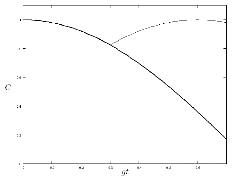
Figure 1: $C\times gt$, without interactions between $M_{b}$ and the atom (thick line) and with an interaction between one atom and $M_{b}$ at $gt=0.3$ (thin line).

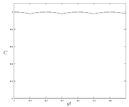
Figure 2: $C\times gt$, with interactions between $M_{b}$ and three atom at $gt=0.1$, $gt=0.2$ and $gt=0.3$ .

References

- (1) R. McDermott, R. W. Simmonds, M. Steffen, K. B. Cooper, K. Cicak, K. D. Osborn, Seongshik Oh, D. P. Pappas, J. M. Martinis, Science 307, 1299 (2005).
- (2) J. P. Reithmaier, G. Sk, A. L ffler, C. Hofmann, S. Kuhn, S. Reitzenstein, L. V. Keldysh, V. D. Kulakovskii, T. L. Reinecke and A. Forchel, Nature 432, 197 (2004).
- (3) G. Nogues, A. Rauschenbeutel, S. Osnaghi, M. Brune, J. M. Raimond and S. Haroche, Nature 400 239 (1999).
- (4) S. Gleyzes, S. Kuhr, C. Guerlin, J. Bernu, S. Del glise, U. Busk Hoff, M. Brune, J.M. Raimond and S. Haroche, Nature 446, 297 (2007).
- (5) P. Bertet, S. Osnaghi, A. Rauschenbeutel, G. Nogues, A. Auffeves, M. Brune, J. M. Raimond and S. Haroche , Nature, 411, 166 (2001).
- (6) M.C.Fischer, B.Gutierrez-Medina and M.G.Raizen, Phys. Rev. Lett. , 87, 040402 (2001).
- (7) M. A. Nielsen and I. L. Chuang, Quantum Computation and Quantum Information (Cambridge University Press, Cambridge, England, 2000).
- (8) Chui-Ping Yang and Shih-I Chu, Phys. Rev. A66, 034301 (2002).
- (9) J. I. Cirac, A. K. Ekert and C. Macchiavello, Phys. Rev. Lett. 82, 4344 (1999).
- (10) L. Viola and S. Lloyd, Phys. Rev. A58, 2733 (1998).
- (11) D. Dhar, L. K. Grover, and S. M. Roy, Phys. Rev. Lett. 96, 100405 (2006).
- (12) B. Misra, E.C. G. Sudarshan, J. Math. Phys. 18, 756 (1977).
- (13) P. Facchi and S. Pascazio, Phys. Rev. Lett. , 89, 080401 (2002).
- (14) J. G. Oliveira Jr, R. Rossi Jr. and M. C. Nemes, Phys. Rev. A, 78, 044301 (2008).
- (15) Sabrina Maniscalco, Francesco Francica, Rosa L. Zaffino, Nicola Lo Gullo, and Francesco Plastina, Phys. Rev. Lett. , 100 090503 (2008).
- (16) R. Rossi, A. R. de Magalh es, and M. C. Nemes, Phys. Rev. A77, 012107 (2008).
- (17) J. M. Raimond, M. Brune, and S. Haroche, Phys. Rev. Lett. 79, 1964 (1997).
- (18) S. Rinner, E. Werner, T. Becker and H. Walther, Phys. Rev. A74 041802 (2006).
- (19) Zhi-Jian Li, Jun-Qi Li, Yan-Hong Jin and Yi-Hang Nie, J. Phys. B 40, 3401 (2007).
- (20) A. Rauschenbeutel, P. Bertet, S. Osnaghi, G. Nogues, M. Brune, J. M. Raimond, and S. Haroche, Phys. Rev. A64, 050301(R) (2001).
- (21) M. Brune, F. Schmidt-Kaler, A. Maali, J. Dreyer, E. Hagley, J. M. Raimond, and S. Haroche, Phys. Rev. Lett. 76, 1800 (1996).