Isospin symmetry breaking

Abstract:

We discuss the separation of isospin-symmetric and isospin-breaking contributions in the hadronic observables within the framework of QCD plus QED. Further, we briefly review some recent work on the low-energy hadron phenomenology, in which the isospin-breaking effect plays a prominent role.

1 Introduction

Strong interactions are described by the Lagrangian of pure QCD, whose only free parameters are the strong coupling constant and the quark masses. Most of theoretical predictions, which are made in the framework of pure QCD, assume, in addition, isospin symmetry, i.e. the masses of the up and down quarks are taken equal. In Nature, however, strong interactions do not come alone: the low-energy processes with the participation of hadrons contain electromagnetic effects – consequently, these processes should be described by the Lagrangian of QCD plus QED (for simplicity, we neglect weak interactions here). Therefore, in order to meaningfully compare the theory with the experiment, one should be able to “purify” experimental data with respect to the isospin-breaking corrections. This task is further complicated with the fact that the perturbation theory can not be applied to describe hadronic processes at low energies and one has to resort to the other techniques, be these the lattice QCD or Chiral Perturbation Theory (ChPT).

Specifically, one faces the following problem. A physical process is described by the Lagrangian of QCD plus QED, whose parameters are the strong coupling constant $g$, the electromagnetic coupling constant $e$ and the (running) quark masses $m_{u},m_{d},m_{s},\cdots$. We define the isospin-symmetric world where $e=0$ and the masses of the up and down quarks are equal. The parameters of the isospin-symmetric world are the strong coupling constant $\bar{g}$ and the quark masses $\bar{m}_{u},\bar{m}_{s},\cdots$, with $\bar{m}_{u}=\bar{m}_{d}$ (the bar over a symbol denotes the isospin-symmetric world). In general, the following questions should be answered:

• How are the parameters $g,e$ and $m_{u},m_{d},m_{s},\cdots$, on the one side, and $\bar{g}$ and $\bar{m}_{u},\bar{m}_{s},\cdots$, on the other side, related?

• How does the separation of isospin-symmetric and isospin-breaking effects translate to the level of the effective chiral Lagrangian, which is used to describe hadronic processes at low energy?

• Once the prescription for separation of the isospin-symmetric and isospin-breaking effects is set, what is the systematic procedure of purifying the hadronic observables with respect to the isospin-breaking corrections?

Recently, some aspects of the problem have been addressed, e.g., in Refs. [1, 2, 3, 4]. Below, we mainly follow the line, adopted in Ref. [3]. Instead of a general reasoning, for illustrative reasons, we concentrate on a particular example.

2 “Purely strong” pion decay constant

In this section, we shall study the question, how to extract the “purely strong” pion decay constant $F_{\pi}$ from experimental data on the decay of a charged pion with 0 or 1 real photon in the final state. This problem has a long history, starting in the pre-ChPT era (see, e.g. [5]). In ChPT, the decay width of this process has been calculated at one [6] and two [7] loops. Below, we give an expression of the decay rate at one loop, evaluated in ChPT with three flavors [6]

$$\Gamma(\pi\to\ell\nu_{\ell}(\gamma)) = \frac{G_{F}^{2}|V_{ud}|^{2}F_{0}^{2}m_{\ell}^{2}M_{\pi^{+}}}{4\pi}\,\biggl{(}1-\frac{m_{\ell}^{2}}{M_{\pi^{+}}^{2}}\biggr{)}^{2}\biggl{\{}1+\frac{8}{F_{0}^{2}}\,(L_{4}^{r}(M_{\pi}^{2}+2M_{K}^{2})+L_{5}^{r}M_{\pi}^{2})$$ (1)

$$- \frac{1}{32\pi^{2}F_{0}^{2}}\,\biggl{(}2M_{\pi^{+}}^{2}\ln\frac{M_{\pi^{+}}^{2}}{\mu^{2}}+2M_{\pi^{0}}^{2}\ln\frac{M_{\pi^{0}}^{2}}{\mu^{2}}+M_{K^{+}}^{2}\ln\frac{M_{K^{+}}^{2}}{\mu^{2}}+M_{K^{0}}^{2}\ln\frac{M_{K^{0}}^{2}}{\mu^{2}}\biggr{)}$$

$$+ e^{2}E^{r}+\frac{e^{2}}{16\pi^{2}}\,\biggl{(}3\ln\frac{M_{\pi}^{2}}{\mu^{2}}+H(\frac{m_{\ell}^{2}}{M_{\pi^{+}}^{2}})\biggr{)}\biggr{\}}\,,$$

where $m_{\ell}$ denotes the lepton mass, $M_{\pi^{+}},M_{\pi^{0}},M_{K^{+}},M_{K^{0}}$ are physical pion and kaon masses, and $M_{\pi}^{2}=2B_{0}\hat{m}$, $M_{K}^{2}=B_{0}(m_{s}+\hat{m})$ with $\hat{m}=\frac{1}{2}\,(m_{u}+m_{d})$. Further, $F_{0}$ denotes the pion decay constant in the chiral limit, $B_{0}$ is proportional to the quark condensate in the chiral limit, $L_{i}^{r}$ denote the strong low-energy constants (LECs), $E^{r}$ is a certain linear combination of the electromagnetic LECs, the function $H(z)$ stands for the contribution of the photon loops, and $\mu$ is the scale of the dimensional regularization. Finally, $G_{F}$ and $V_{ud}$ stand for the Fermi constant and the element of the Cobayashi-Maskawa matrix.

The reasoning goes as follows. In the isospin-symmetric world, the quantity $F_{0}$ can be related to the charged pion decay constant $F_{\pi}$ through the well-known expression [8]

$$F_{\pi}=F_{0}\biggl{\{}1+\frac{4}{F_{0}^{2}}\,(L_{4}^{r}(M_{\pi}^{2}+2M_{K}^{2})+L_{5}^{r}M_{\pi}^{2})-\frac{1}{32\pi^{2}F_{0}^{2}}\,\biggl{(}2M_{\pi}^{2}\ln\frac{M_{\pi}^{2}}{\mu^{2}}+M_{K}^{2}\ln\frac{M_{K}^{2}}{\mu^{2}}\biggr{)}\biggr{\}}\,.$$ (2)

Here one has implicitly assumed that passing to the isospin limit amounts to setting $e=0$, $m_{d}=m_{u}=\hat{m}$, whereas all other parameters of the theory stay put. Further, substituting this expression into Eq. (1), it is seen that one may extract the exact value of $F_{\pi}$ from the measured value of the decay rate, provided one makes reliable estimates for the electromagnetic LECs contained in $E^{r}$.

In order to demonstrate that this procedure is ambiguous in general, we calculate the pion decay constant in a model where, unlike QCD, explicit calculations can be performed. To this end, we invoke the linear $\sigma$-model to one loop. In the limit when the mass of $\sigma$ becomes much larger than the pion mass, the low-energy structure of the theory can be described by ChPT – with the specific values of the LECs which are determined by the underlying Lagrangian of the $\sigma$-model.

In the following, we mainly follow Ref. [3]. The Lagrangian of the linear $\sigma$-model with electromagnetic interactions is given by ${\cal L}={\cal L}_{0}+{\cal L}_{\sf ct}$, where

$${\cal L}_{0} = \frac{1}{2}\,d_{\mu}\phi^{T}d^{\mu}\phi+\frac{m^{2}}{2}\,\phi^{T}\phi-\frac{g}{4}\,(\phi^{T}\phi)^{2}+c\phi^{0}+\frac{\delta m^{2}}{2}\,(Q\phi)^{T}(Q\phi)$$ (3)

$$- \frac{\delta g}{2}\,(Q\phi)^{T}(Q\phi)(\phi^{T}\phi)-\frac{1}{4}\,F_{\mu\nu}F^{\mu\nu}-\frac{1}{2\xi}\,(\partial_{\mu}A^{\mu})^{2}\,,$$

where $\phi\doteq(\phi^{0},\phi^{i})$ denotes the 4-component spin-0 field, $A_{\mu}$ is the electromagnetic field, $F_{\mu\nu}$ is the electromagnetic field tensor, $\xi$ is the gauge parameter and $Q$ stands for the $4\times 4$ charge matrix, whose non-zero components are $Q_{12}=-Q_{21}=1$. Further, the covariant derivative of the field $\phi$ is defined as $d^{\mu}\phi=\partial^{\mu}\phi+(F^{\mu}+eQA^{\mu})\phi$, where external vector and axial-vector fields are given by $F_{\mu}^{0i}=a_{\mu}^{i}\,,\quad F_{\mu}^{ij}=-\epsilon^{ijk}v_{\mu}^{k}$. Finally, the counterterm Lagrangian ${\cal L}_{\sf ct}=\sum_{a=1}^{8}\beta_{a}{\cal O}_{a}$ includes all operator structures, which are necessary to remove divergences to one loop (for more details, see Ref. [3]). The isospin-breaking parameters parameters $\delta m^{2},\delta g$ are counted at order $e^{2}$.

The spontaneous chiral symmetry breaking in the model occurs, when $m^{2}>0$. In this case, the parameter $c$, which describes the explicit breaking of chiral symmetry, determines the mass of the neutral pion (the charged pion mass receives an additional piece proportional to $e^{2}$, see [3]). The mass of the $\sigma$-meson, $M_{\sigma}$, does not vanish in the chiral limit.

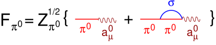
Figure 1: The neutral pion decay constant at one loop in the linear $\sigma$-model.

In order to evaluate the pion decay constant, we calculate the matrix element of an axial current between the vacuum and the neutral pion state to one loop. This matrix element is determined by the diagrams shown in Fig. 1. At the next step, we perform the limit $M_{\sigma}\to 0$ in the resulting expressions, and compare the answer with the neutral pion decay constant, calculated in the two-flavor ChPT [9]

$$F_{\pi^{0}}=F\biggl{\{}1-\frac{M_{\pi^{+}}^{2}}{16\pi^{2}F^{2}}\,\ln\frac{M_{\pi^{+}}^{2}}{\mu^{2}}+\frac{M_{\pi^{0}}^{2}}{F^{2}}\,l_{4}^{r}-e^{2}\sum_{i}c_{i}k_{i}^{r}\biggr{\}}\,,$$ (4)

where $F,l_{i}^{r}$ are the $SU(2)$-analogs of $F_{0},L_{i}^{r}$, and $c_{i}k_{i}^{r}$ stands for a some linear combination of the electromagnetic LECs. The matching gives

$$F(1-e^{2}\sum_{i}c_{i}k_{i}^{r})=\frac{m}{\sqrt{g}}\,\biggl{\{}1-\frac{3g}{16\pi^{2}}\,\ln\frac{2m^{2}}{\mu^{2}}+\frac{7g}{32\pi^{2}}\biggr{\}}\,.$$ (5)

Now, we must move one step further and relate the quantity $F$ to its “purely strong” counterpart, defined in the limit $e=0$. This procedure is straightforward in Quantum Mechanics but becomes obscure in the framework of the Quantum Field Theory, where one has to deal with the renormalized parameters. The renormalization group (RG) equations, which govern the running of these parameters, to one loop are given by (see Ref. [3])

$$\mu\frac{dm^{2}}{d\mu} = \frac{1}{4\pi^{2}}\,((3g+\delta g)m^{2}+g\,\delta m^{2})$$ (6)

$$\mu\frac{dg}{d\mu} = \frac{1}{2\pi^{2}}\,(3g^{2}+g\,\delta g)$$ (7)

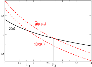
Figure 2: Matching of the strong coupling constant in full theory and in case when the electromagnetic interactions are switched off. The figure illustrates the uncertainty related to the choice of the matching scale.

Whereas the RG equations in the isospin-symmetric world are obtained by setting $e=0$ in Eq. (6)

$$\mu\frac{d\bar{m}^{2}}{d\mu} = \frac{3}{4\pi^{2}}\,\bar{g}\bar{m}^{2}\,,$$ (8)

$$\mu\frac{d\bar{g}}{d\mu} = \frac{3}{2\pi^{2}}\,\bar{g}^{2}\,.$$ (9)

The crucial point here is that the procedure of switching off the electromagnetic corrections unambiguously predicts the running of the parameters with respect to the renormalization scale $\mu$, but not the value of these parameters at a given $\mu$. The parameters $g(\mu)$, $m^{2}(\mu)$ can be, in principle, fixed from the experimental data. However, this is impossible for $\bar{g}(\mu)$, $\bar{m}^{2}(\mu)$, since there are no data with electromagnetic interactions switched off. For this, in order to fix the values of $\bar{g}(\mu)$, $\bar{m}^{2}(\mu)$, one has to invoke additional conventions, rendering the definition of the isospin-symmetric limit convention-dependent. For example, one may impose boundary condition on the solutions of Eq. (8) at some $\mu=\mu_{1}$ which will be hereafter referred to as the matching scale. Most easily, this can be done by requiring $g(\mu_{1})=\bar{g}(\mu_{1})$ and $m^{2}(\mu_{1})=\bar{m}^{2}(\mu_{1})$. Then, from Eqs. (6) and (8) one obtains

$$m^{2}(\mu) = \bar{m}^{2}(\mu;\mu_{1})+\frac{1}{4\pi^{2}}\,\ln\frac{\mu}{\mu_{1}}\,(\delta g\,m^{2}+g\,\delta m^{2})\,,$$ (10)

$$g(\mu) = \bar{g}(\mu;\mu_{1})+\frac{1}{2\pi^{2}}\,\ln\frac{\mu}{\mu_{1}}\,g\,\delta g\,.$$ (11)

Here, we explicitly indicate the $\mu_{1}$-dependence of the parameters of the theory in the isospin symmetry limit. This dependence is illustrated in Fig. 2 where it is shown that, changing the matching scale from $\mu_{1}$ to $\mu_{2}$ leads to the change of the value of $\bar{g}(\mu)$ at a fixed $\mu$.

From Eq. (5) one now obtains (remember that the quantity $F$, by definition, refers to the isospin-symmetric world)

$$F=\frac{\bar{m}}{\sqrt{\bar{g}}}\,\biggl{\{}1-\frac{3\bar{g}}{16\pi^{2}}\,\ln\frac{2\bar{m}^{2}}{\mu^{2}}+\frac{7\bar{g}}{32\pi^{2}}\biggr{\}}\,.$$ (12)

One may directly check that $\mu\frac{dF}{d\mu}=0$, as it should. However, the quantity $F$ depends on the choice of the matching scale since $\mu_{1}\frac{dF}{d\mu_{1}}\neq 0$. This is the ambiguity inherent to the definition of the isospin-symmetry limit. There is no way to avoid this ambiguity. On the other hand, a particular combination of $F$ and the electromagnetic LECs, which is present in Eq. (5), is free of this ambiguity.

It turns out that within the framework of the linear $\sigma$-model it is possible to make a numerical estimate of the size of this uncertainty. This happens because the quantities $\delta g$ and $\delta m^{2}$, which determine the $\mu_{1}$ dependence of the parameters in Eq. (10), also enter the expression of the charged and neutral pion mass difference. Using this fact, one obtains the following estimate within the linear $\sigma$-model [3]

$$F(\mu_{1}=1~{}\mbox{GeV})-F(\mu_{1}=0.5~{}\mbox{GeV})\simeq 0.1~{}\mbox{MeV}\,.$$ (13)

That shows that the effect is not purely academic (for example, one may compare this with the uncertainty in $F_{\pi}$, quoted recently in Ref. [10]).

The following conclusions can be drawn:

• The separation of the electromagnetic and strong interactions is not an unambiguous operation in Quantum Field Theory. We have seen this explicitly on the example of the linear $\sigma$-model at one loop, and we have no reason to believe that this will be different in QCD.

• As explained above, this ambiguity can be fixed, e.g., by setting boundary conditions in the RG equation. As a result, the parameters of the isospin-symmetric theory will depend on the choice if the matching scale $\mu_{1}$. Alternatively, one may use observable quantities for fixing the ambiguity. In the example considered in this section, it suffices to set the pion decay constant and the pion and the $\sigma$ masses in the isospin-symmetric world to a given values (known as reference values). This determines the quantities $\bar{g}$, $\bar{m}^{2}$ and $c$ uniquely. All other observables are expressed through these parameters.

• Returning to the issue of extracting the value of $F_{\pi}$ from the data, we see that the extraction with an arbitrarily high precision is not possible, because the quantity $F$ (and hence $F_{\pi}$ which coincides with $F$ in the chiral limit) depends on the matching scale $\mu_{1}$.

• Using ChPT with virtual photons, which was originally introduced in Refs. [11, 12], to calculate isospin-breaking corrections to the “purely hadronic” observables implies that the hadronic LECs stay put in the isospin symmetry limit. In the linear $\sigma$-model this means that the LECs are expressed through $\bar{g}$ and $\bar{m}^{2}$, so that they depend on $\mu_{1}$. On the other hand, the physical quantities in the real world do not depend on $\mu_{1}$. Consequently, the $\mu_{1}$-dependence in the strong LECs must be compensated by a redefinition of the electromagnetics LECs. In the example with extracting $F_{\pi}$ from the data this would mean that there exists an inherent uncertainty which does not allow us to fix the electromagnetic LECs – and hence $F_{\pi}$ – with an arbitrary precision.

3 Isospin-breaking effects in hadronic observables

From the previous section one may conclude that the definition of the (hypothetic) isospin-symmetric world, which sets the reference point for the calculation of the isospin-breaking corrections, is ambiguous. On the other hand, there exist observable isospin-breaking effects, where the above ambiguity does not matter. Below, we want to briefly review some recent work where the isospin-breaking effects play a prominent role, and highlight the issues which are related to the discussion given in the previous section.

3.1 Cusps in the $K\to 3\pi$ decays

Recently, NA48/2 collaboration at CERN observed a pronounced Wigner cusp [13] in the invariant mass distribution for the three-pion decays of charged kaons [14]. Cabibbo in Ref. [15] proposed that measuring this cusp, which is due to the presence of the charged and neutral pion mass difference, can be used for extracting the values of the $\pi\pi$ scattering lengths (originally, the cusp has been predicted in Ref. [16], see also [17] where the cusp in the $\pi\pi$ scattering amplitude is discussed). However, the accuracy of the one-loop representation of the $K\to 3\pi$ decay amplitudes, which is given in Ref. [15], does not suffice to fit the high-precision experimental data. To this end, in Ref. [18] one has used analyticity and unitarity of the $S$-matrix to obtain a theoretical representation of the charged and neutral kaon decay amplitudes, valid up to and including second order in the $\pi\pi$ scattering lengths. The authors of Ref. [19] have merged the above approach with ChPT, which is only used to calculate the real part of the $K\to 3\pi$ decay amplitude at one loop. In Ref. [20], the charged pion decays have been studied to the same accuracy within the non-relativistic effective Lagrangian approach, which turns out to be a most systematic and convenient tool to address the problem. In particular, it automatically includes the strictures imposed by analyticity and unitarity. Furthermore, the inclusion of the electromagnetic effects proceeds straightforwardly within this approach [21]. Using two-loop representation of the decay amplitudes, a precise determination of the $\pi\pi$ scattering lengths is possible [22]. Finally, we mention two more approaches to the same problem. Ref. [23] uses the dispersive approach. Recently, there have been attempts [24] to address the problem in a framework which may be considered as a merger between $K$-matrix theory and a conventional quantum-mechanical framework used to study Coulomb interactions in the final state. In general, this framework is contradictory and incomplete, since, e.g., it fails to reproduce the correct two-loop structure of the decay amplitude, as well as the full set of isospin-breaking corrections to it.

It should be pointed out that the non-relativistic approach can be straightforwardly generalized to study other three-particle decays, like the decays of the neutral kaons [25], (for the experiments on neutral kaons, see Refs. [14, 26]), as well as $\eta\to 3\pi$ decays [27] and $\eta^{\prime}\to\eta 2\pi$ decays [28]. From the recent developments, we also highlight a comprehensive calculation of the isospin-breaking corrections at order $e^{2}(m_{d}-m_{u})$ in $\eta\to 3\pi$ decays, carried out in ChPT to one loop [29]. These calculations complement earlier calculations at order $e^{2}\hat{m}$, carried out in Ref. [30]. For more theoretical and experimental developments on the cusps, see, e.g., contributions to this workshop [22, 31].

We would like to stress that the representation of the decay amplitude, which is considered in the present subsection, concerns the real world and the observable isospin-breaking effects (like the emerging cusp) only. No reference is made to the idealized world with no isospin breaking until the very end, when the relation between the physical $\pi\pi$ scattering amplitudes in different channels and the $S$-wave $\pi\pi$ scattering lengths $a_{0},a_{2}$ is established (see Ref. [20] for more detail). Fortunately, the isospin-breaking corrections, contained in this relation, at leading order can be expressed by the charged and neutral pion mass difference and are thus parameter-free [20]. The electromagnetic LECs, which are the source of ambiguity discussed in the previous section, appear only at next-to-leading order. Their contribution are expected to be small and well-controlled.

Finally, we would like to emphasize that ChPT [32], combined with Roy equations, allows one to make very precise predictions for the values of the S-wave scattering lengths in elastic $\pi\pi$ scattering [33]. For this reason, confronting the experimental results with these predictions, one may extract important information about the fundamental properties of QCD at low energy. For instance, the above predictions for the scattering lengths have been made in the assumption that the spontaneous chiral symmetry breaking in QCD proceeds according to the standard scenario (with the large quark condensate). If the experimentally measured scattering lengths significantly deviate from the theoretically predicted values, this would indicate that the symmetry breaking in QCD follows a different path.

3.2 Isospin-breaking corrections is $K_{e4}$ decays

$K_{e4}$ decays represent an important source for the determination of the $\pi\pi$ scattering phase shift and scattering lengths [34, 35, 22]. The crucial observation which allows one to link the $K_{e4}$ decay amplitude to the $\pi\pi$ elastic scattering amplitude is that, according to the Watson theorem, the phases of both amplitudes coincide. Watson theorem, however, assumes isospin symmetry, which is violated in Nature. It is therefore justified to ask, how large are the corrections in the $\pi\pi$ scattering phase, which is extracted from the $K_{e4}$ decays.

In fact, in the analysis of the experimental data one has already removed part of these corrections, applying the Coulomb factor and using the program PHOTOS [36] – see Ref. [35] for details. This procedure definitely leaves out some of the isospin-breaking corrections, e.g., those caused by the mass differences in the isospin multiplets, or direct effects related to the quark mass difference $m_{d}-m_{u}$. Thus, one is faced with an alternative: either one chooses to deal with the “raw” experimental data and removes a full set of isospin-breaking corrections which can be systematically calculated in ChPT, or one uses the data already “corrected” by PHOTOS and removes additional isospin-breaking effects, assuming that this can be done separately. Although the first option is definitely more appealing, it requires a major calculational effort (see Ref. [37] for an earlier work in this direction). Recently, the calculation of the isospin-breaking corrections, using the “corrected” data, has been carried out in Ref. [38] (see also Refs. [39] which attempt to calculate the effects caused by the pion mass splitting and electromagnetic corrections). The findings of Ref. [38] can be summarized as follows:

• The isospin-breaking correction have been calculated to one loop in ChPT. Virtual photons have been neglected. The charged pion mass is used as the reference mass for the isospin symmetric world. Both the corrections coming from the pion mass difference and the effect proportional to $m_{d}-m_{u}$, which originates from the $\pi^{0}-\eta$ mixing phenomenon, are taken into account. Both these effects are of a comparable size.

• Watson theorem holds only in case of isospin symmetry. When isospin symmetry is violated, the phases in the $K_{e4}$ decay amplitude and in the $\pi\pi$ elastic amplitude differ. Moreover, they are not related to each other: for example, the decay amplitude contains some electromagnetic LECs which are not present in the $\pi\pi$ amplitude.

• If isospin symmetry is violated, the phase of the $K_{e4}$ decay amplitude has a cusp below threshold. The phase no more vanishes at threshold $s=4M_{\pi^{+}}^{2}$.

• It has been shown that the isospin breaking effect is quite large (see Fig. 3). Moreover, these corrections strongly affect the values of the S-wave $\pi\pi$ scattering lengths, which are extracted from the experimental data [22]. Only after the isospin breaking is taken into account, the experimental output for the scattering lengths agrees with the theoretical prediction [33].

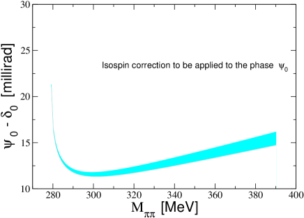
Figure 3: The difference between the phase in the $K_{e4}$ amplitude $\psi_{0}$ and the $\pi\pi$ elastic S-wave scattering phase with full isospin $I=0$ in the isospin limit $\delta_{0}$. The blue band shows the error caused by the uncertainty in the parameters of the calculation. $M_{\pi\pi}$ denotes the invariant mass of the charged pion pair.

3.3 Isospin breaking in the $\pi N$ scattering and in the pionic hydrogen observables

The experiments on hadronic atoms [40, 41, 42] provide a beautiful possibility to directly extract the hadron-hadron scattering lengths from the experimental data without using the extrapolation to the threshold. However, the accuracy of the extraction of the scattering lengths critically depends on the possibility to gain a control on the isospin breaking corrections in the atomic observables.

In Ref. [43] the relation of the ground-state energy level shift in the pionic hydrogen and the elastic $\pi^{-}p$ threshold scattering amplitude is obtained at next-to-leading order in isospin breaking. Further, in Ref. [44] a similar relation between the width of the ground state and the charge-exchange $\pi^{-}p\to\pi^{0}n$ threshold amplitude has been derived. The accuracy of these relations comfortably matches the existing experimental precision. However, the question of calculating the isospin-breaking corrections for the threshold amplitudes, in order to relate these quantities to the S-wave $\pi N$ scattering lengths, has proven to be more difficult. One invokes ChPT to this end. In Ref. [43], the isospin-breaking corrections to the $\pi^{-}p$ amplitude has been obtained at $O(p^{2})$, using the charged pion and proton masses as reference masses in the isospin-symmetric world. In Ref. [45] these calculations have been extended to $O(p^{3})$. Finally, in Ref. [44] the isospin-breaking corrections to the charge-exchange amplitude have been evaluated at $o(p^{2})$. For the recent review on the subject, see, e.g., [46, 47].

There are, generally, two problems, related to the calculation of these corrections:

• Using leading order values for the corrections does not always suffice. Loop corrections can be sizable, see, e.g., Ref. [45].

• The lowest-order LECs (most notably, the electromagnetic LECs) are poorly known. Entering the result already at leading order, these LECs are responsible for the bulk of the uncertainty in the calculations.

Although the calculations at higher orders in ChPT can not improve on item ii), they can definitely check the convergence of the chiral expansion and lead to a more reliable estimate of the isospin breaking corrections, see item i). This is the major justification for the comprehensive study of the isospin-breaking effect in all physical $\pi N$ scattering amplitudes at threshold, which has been undertaken in Ref. [48] at $O(p^{3})$ in the relativistic baryon ChPT. A careful analysis given in Ref. [48], which involved both extensive analytic calculations and a significant numerical effort, will allow one to carry out the extraction of the $\pi N$ scattering lengths from the pionic hydrogen data in a more controllable manner.

4 Acknowledgments

The author would like to thank Jürg Gasser for numerous interesting discussions. This research is part of the EU HadronPhysics2 project “Study of strongly interacting matter” under the Seventh Framework Programme of EU (Grant agreement n. 227431). Work supported in part by DFG (SFB/TR 16, “Subnuclear Structure of Matter”), by the Helmholtz Association through funds provided to the virtual institute “Spin and strong QCD” (VH-VI-231) and by the grant of Georgia National Science Foundation (Grant # GNSF/ST08/4-401).

References

- [1] J. Bijnens, Phys. Lett. B 306, 343 (1993) [arXiv:hep-ph/9302217]; J. Bijnens and J. Prades, Nucl. Phys. B 490 (1997) 239 [arXiv:hep-ph/9610360].
- [2] B. Moussallam, Nucl. Phys. B 504 (1997) 381 [arXiv:hep-ph/9701400], B. Ananthanarayan and B. Moussallam, JHEP 0406 (2004) 047 [arXiv:hep-ph/0405206].
- [3] J. Gasser, A. Rusetsky and I. Scimemi, Eur. Phys. J. C 32 (2003) 97 [arXiv:hep-ph/0305260].
- [4] J. Gegelia, Eur. Phys. J. A 19 (2004) 355 [arXiv:nucl-th/0310012].
- [5] T. Kinoshita, Phys. Rev. Lett. 2 (1959) 477; S. M. Berman, Phys. Rev. Lett., 50 (1958) 468; A. Bailin, D. Bailin, Nuovo Cim., 69 (1970) 207; A. Sirlin, Phys. Rev. D 5 (1972) 436; M.V. Terent’ev, Sov. J. Nucl. Phys. 18 (1974) 709; W. J. Marciano and A. Sirlin, Phys. Rev. Lett. 36 (1976) 1425; T. Goldman, W. J. Wilson, Phys. Rev. D 15 (1977) 709; M. Finkemeier, Phys. Lett. B 387 (1996) 391 [arXiv:hep-ph/9505434]; W. J. Marciano and A. Sirlin, Phys. Rev. Lett. 71 (1993) 3629.
- [6] M. Knecht, H. Neufeld, H. Rupertsberger and P. Talavera, Eur. Phys. J. C 12 (2000) 469 [arXiv:hep-ph/9909284].
- [7] V. Cirigliano and I. Rosell, JHEP 0710 (2007) 005 [arXiv:0707.4464 [hep-ph]]; I. Rosell, a contribution this workshop.
- [8] J. Gasser and H. Leutwyler, Nucl. Phys. B 250 (1985) 465.
- [9] M. Knecht and R. Urech, Nucl. Phys. B 519 (1998) 329 [arXiv:hep-ph/9709348].
- [10] B. Ananthanarayan and B. Moussallam, JHEP 0205 (2002) 052 [arXiv:hep-ph/0205232].
- [11] R. Urech, Nucl. Phys. B 433 (1995) 234 [arXiv:hep-ph/9405341].
- [12] H. Neufeld and H. Rupertsberger, Z. Phys. C 71 (1996) 131 [arXiv:hep-ph/9506448].
- [13] E. P. Wigner, Phys. Rev. 73 (1948) 1002.
- [14] J. R. Batley et al. [NA48/2 Collaboration], Phys. Lett. B 633 (2006) 173 [arXiv:hep-ex/0511056].
- [15] N. Cabibbo, Phys. Rev. Lett. 93 (2004) 121801 [arXiv:hep-ph/0405001].
- [16] P. Budini and L. Fonda, Phys. Rev. Lett. 6 (1961) 419.
- [17] U.-G. Meißner, G. Müller and S. Steininger, Phys. Lett. B 406 (1997) 154 [Erratum-ibid. B 407 (1997) 454] [arXiv:hep-ph/9704377].
- [18] N. Cabibbo and G. Isidori, JHEP 0503 (2005) 021 [arXiv:hep-ph/0502130].
- [19] E. Gámiz, J. Prades and I. Scimemi, Eur. Phys. J. C 50 (2007) 405 [arXiv:hep-ph/0602023].
- [20] G. Colangelo, J. Gasser, B. Kubis and A. Rusetsky, Phys. Lett. B 638 (2006) 187 [arXiv:hep-ph/0604084].
- [21] M. Bissegger, A. Fuhrer, J. Gasser, B. Kubis and A. Rusetsky, Nucl. Phys. B 806 (2009) 178 [arXiv:0807.0515 [hep-ph]].
- [22] B. Bloch-Devaux, PoS CONFINEMENT8 (2008) 029; B. Bloch, a contribution to this workshop.
- [23] M. Zdrahal, K. Kampf, M. Knecht and J. Novotny, arXiv:0905.4868 [hep-ph].
- [24] S. R. Gevorkyan, A. V. Tarasov and O. O. Voskresenskaya, Phys. Lett. B 649 (2007) 159 [arXiv:hep-ph/0612129]; arXiv:0910.3904 [hep-ph]; S. R. Gevorkyan, D. T. Madigozhin, A. V. Tarasov and O. O. Voskresenskaya, Phys. Part. Nucl. Lett. 5 (2008) 85 [arXiv:hep-ph/0702154].
- [25] M. Bissegger, A. Fuhrer, J. Gasser, B. Kubis and A. Rusetsky, Phys. Lett. B 659 (2008) 576 [arXiv:0710.4456 [hep-ph]].
- [26] E. Abouzaid et al. [KTeV Collaboration], Phys. Rev. D 78 (2008) 032009 [arXiv:0806.3535 [hep-ex]].
- [27] C. O. Gullstrom, A. Kupsc and A. Rusetsky, Phys. Rev. C 79 (2009) 028201 [arXiv:0812.2371 [hep-ph]].
- [28] B. Kubis and S. P. Schneider, Eur. Phys. J. C 62 (2009) 511 [arXiv:0904.1320 [hep-ph]].
- [29] C. Ditsche, B. Kubis and U.-G. Meißner, Eur. Phys. J. C 60 (2009) 83 [arXiv:0812.0344 [hep-ph]].
- [30] R. Baur, J. Kambor and D. Wyler, Nucl. Phys. B 460 (1996) 127 [arXiv:hep-ph/9510396].
- [31] S. Giudici, C. Ditsche, A. Kupsc, S. Lanz, S. Prakhov, S. P. Schneider, M. Zdrahal, contributions to this workshop.
- [32] S. Weinberg, Physica A 96 (1979) 327; J. Gasser and H. Leutwyler, Annals Phys. 158 (1984) 142.
- [33] G. Colangelo, J. Gasser and H. Leutwyler, Nucl. Phys. B 603 (2001) 125 [arXiv:hep-ph/0103088].
- [34] L. Rosselet et al., Phys. Rev. D 15 (1977) 574; S. Pislak et al. [BNL-E865 Collaboration], Phys. Rev. Lett. 87 (2001) 221801 [arXiv:hep-ex/0106071]; Phys. Rev. D 67 (2003) 072004 [arXiv:hep-ex/0301040].
- [35] J. R. Batley et al. [NA48/2 Collaboration], Eur. Phys. J. C 54 (2008) 411.
- [36] E. Barberio, B. van Eijk and Z. Was, Comput. Phys. Commun. 66 (1991) 115; E. Barberio and Z. Was, Comput. Phys. Commun. 79 (1994) 291; G. Nanava and Z. Was, Eur. Phys. J. C 51 (2007) 569 [arXiv:hep-ph/0607019].
- [37] A. Nehme, Phys. Rev. D 70 (2004) 094025 [arXiv:hep-ph/0406209]; J. Bijnens and F. Borg, Eur. Phys. J. C 39 (2005) 347 [arXiv:hep-ph/0410333]; Eur. Phys. J. C 40 (2005) 383 [arXiv:hep-ph/0501163].
- [38] G. Colangelo, J. Gasser and A. Rusetsky, Eur. Phys. J. C 59 (2009) 777 [arXiv:0811.0775 [hep-ph]].
- [39] S. R. Gevorkyan, A. N. Sissakian, A. V. Tarasov, H. T. Torosyan and O. O. Voskresenskaya, arXiv:0704.2675 [hep-ph]; arXiv:0711.4618 [hep-ph]; Yu. M. Bystritskiy, S. R. Gevorkyan and E. A. Kuraev, arXiv:0906.0516 [hep-ph].
- [40] B. Adeva et al. [DIRAC Collaboration], J. Phys. G 30 (2004) 1929 [arXiv:hep-ex/0409053]; D. Goldin [DIRAC Collaboration], Int. J. Mod. Phys. A 20 (2005) 321; B. Adeva et al. [DIRAC Collaboration], Phys. Lett. B 619 (2005) 50 [arXiv:hep-ex/0504044]; B. Adeva et al., Lifetime measurement of and atoms to test low energy QCD. Addendum to the DIRAC proposal, CERN-SPSC-2004-009 [SPSC-P-284 Add.4].
- [41] D. Gotta [Pionic Hydrogen Collaboration], Int. J. Mod. Phys. A 20 (2005) 349; L. M. Simons [Pionic Hydrogen Collaboration], Int. J. Mod. Phys. A 20 (2005) 1644; D. Gotta, Prog. Part. Nucl. Phys. 52 (2004) 133.
- [42] G. Beer et al. [DEAR Collaboration], Phys. Rev. Lett. 94 (2005) 212302; J. Zmeskal et al., Nucl. Phys. A 754 (2005) 369; C. Curceanu-Petrascu et al., Eur. Phys. J. A 31 (2007) 537; V. Lucherini, Int. J. Mod. Phys. A 22 (2007) 221.
- [43] V. E. Lyubovitskij and A. Rusetsky, Phys. Lett. B 494 (2000) 9 [arXiv:hep-ph/0009206].
- [44] P. Zemp, Deser-type formula for pionic hydrogen, talk given at: Workshop “Hadronic Atoms”, October 13–17, 2003, ECT⋆, Trento, Italy, in: Proceedings “HadAtom03”, Eds. J. Gasser, A. Rusetsky, J. Schacher, p.18 [arXiv:hep-ph/0401204]; P. Zemp, Pionic Hydrogen in QCD+QED: Decay width at NNLO, PhD thesis, University of Bern, 2004.
- [45] J. Gasser, M. A. Ivanov, E. Lipartia, M. Mojžiš and A. Rusetsky, Eur. Phys. J. C 26 (2002) 13 [arXiv:hep-ph/0206068].
- [46] J. Gasser, V. E. Lyubovitskij and A. Rusetsky, Phys. Rept. 456 (2008) 167 [arXiv:0711.3522 [hep-ph]].
- [47] J. Gasser, V. E. Lyubovitskij and A. Rusetsky, Ann. Rev. Part. Nucl. Sci. (in print), arXiv:0903.0257 [hep-ph].
- [48] M. Hoferichter, B. Kubis and U. G. Meissner, Phys. Lett. B 678 (2009) 65 [arXiv:0903.3890 [hep-ph]]; M. Hoferichter, a contribution to this workshop.