Geodesics and flows in a Poissonian city

Abstract

The stationary isotropic Poisson line process was used to derive upper bounds on mean excess network geodesic length in Aldous and Kendall [Adv. in Appl. Probab. 40 (2008) 1–21]. The current paper presents a study of the geometry and fluctuations of near-geodesics in the network generated by the line process. The notion of a “Poissonian city” is introduced, in which connections between pairs of nodes are made using simple “no-overshoot” paths based on the Poisson line process. Asymptotics for geometric features and random variation in length are computed for such near-geodesic paths; it is shown that they traverse the network with an order of efficiency comparable to that of true network geodesics. Mean characteristics and limiting behavior at the center are computed for a natural network flow. Comparisons are drawn with similar network flows in a city based on a comparable rectilinear grid. A concluding section discusses several open problems.

60D05, 90B15, Dufresne integral, frustrated optimization, geometric spanner network, growth process, improper anisotropic Poisson line process, Lamperti transformation, Laplace exponent, Levy process, logarithmic excess, Manhattan city network, Mills ratio, mark distribution, martingale central limit theorem, network geodesic, Palm distribution, perpetuity, Poisson line process, Poissonian city network, Slivynak theorem, spanner, spatial network, subordinator, traffic flow, uniform integrability

1 Introduction

The “Poissonian city” is a random network of connections based on a Poisson line process. Aldous and Kendall (2008) used such a network to address a problem in frustrated optimization: construct planar networks connecting a large number of nodes such that:

1. the total connection length is not much larger than the minimum possible connection length, but also such that

2. the average connection distance between two randomly chosen nodes is not greatly in excess of the Euclidean distance.

It transpires that networks satisfying criterion 1 may be augmented by sparse Poisson line processes so as to satisfy criterion 2 as well. More precisely, suppose that $n$ nodes are distributed in an arbitrary fashion (deterministically or randomly) over a square of total area $n$. Recall that the minimum total length for a connecting network is achieved by a Steiner minimum tree [Prömel and Steger (2002) survey Steiner trees in general; for probabilistic aspects, see Steele (1997), Yukich (1998)]. It is shown by Aldous and Kendall [(2008), Theorem 1(b)] that augmentation by a sparse Poisson line process can convert a Steiner minimum tree into a network whose total connection length is only slightly increased but which now delivers a mean connection distance that is no more than $O(\log n)$ in excess of the Euclidean distance. (Here, the mean involves averaging the choice of nodes rather than the randomness of the line process.) Under a suitable weak uniformity condition on the empirical spatial distribution of the nodes, Aldous and Kendall [(2008), Theorem 2] also establish a lower bound on the mean excess: it must be of order at least $\Omega(\sqrt{\log n})$.

The primary motivation of the previously mentioned work was to gain a better understanding of the behavior of network statistics (such as the mean excess network length) for entirely general networks. However, the appearance of Poisson line processes in the upper bound result motivates the following, more detailed, study of the “Poissonian city” generated by a unit intensity stationary isotropic Poisson line process. What can be said about the “near-geodesics” used to establish the upper bound? How close are they to true network geodesics? How does random fluctuation affect excess length? And what about traffic flow on such a network? These questions are addressed below; their answers require the use of Lévy subordinators, self-similar Markov processes (something of a novelty in stochastic geometry) and a curious improper anisotropic Poisson line process.

Previous relevant work includes: the note by Davidson (1974), who gives a qualitative argument showing that the Poisson line process provides good connections; Rényi and Sulanke [(1968), Satz 5], who derive a result similar to the mean-excess result, but concerning numbers of edges rather than length, and based on a fixed number of random lines; and recent higher-dimensional generalizations of the Rényi–Sulanke work by Böröczky and Schneider (2010), Theorem 1.3. We also mention work by Voss, Gloaguen and Schmidt (2009) on limit distributions of shortest paths from subsidiary to major nodes in hierarchical networks based on random tessellations. Finally, we note the interesting work of Baccelli, Tchoumatchenko and Zuyev (2000) related to the concept of spanners from graph theory [a geometric spanner is a planar graph connecting a set of nodes for which the graph distance between any two points is less than some fixed multiple of Euclidean distance; see, e.g., the exposition Narasimhan and Smid (2007)]. The networks constructed in Aldous and Kendall (2008) are averaged rather than uniform versions of geometric spanner networks, for which the fixed multiple of Euclidean distance is replaced by a logarithmic additive excess and a specific constraint is imposed on the total network length (rather than, say, small vertex degree or total number of edges).

In the remainder of this introductory section we introduce basic notation and concepts, and enumerate the questions to be addressed concerning the behavior of near-geodesics and traffic flow in the Poissonian city.

1.1 Notation and basic concepts

We begin by presenting a brief summary of stationary isotropic Poisson line processes so as to fix notation and collect some facts about line processes which will be used below. Further information can be found in, for example, Stoyan, Kendall and Mecke (1995). The ensemble of undirected lines $\ell$ in the plane may be viewed as a Möbius strip of infinite width or as a once-punctured projective plane (since such lines can be produced as intersections of planes through the origin in $3$-space with the plane $z=1$, in which case the plane through the origin and parallel to $z=1$ does not produce an intersection). It is often convenient to parametrize this ensemble of lines $\ell$ by representing lines using points $(r,\theta)$, where $r$ is the perpendicular signed distance from the line $\ell$ to a reference point, and $\theta\in[0,\pi)$ is the angle that $\ell$ makes with a reference line running through the reference point. A unit intensity stationary isotropic Poisson line process (“Poisson line process” for short) is determined as a Poisson point process on the representing projective plane using the intensity measure $\frac{1}{2}\,{{d}}r\,{d}\theta$. The factor $\frac{1}{2}$ ensures that the mean number of Poisson lines hitting a line segment is equal to the length of the segment.

Slivynak’s theorem on the Palm distribution of a Poisson process applies here: if we condition on a specific line $\ell$ belonging to the Poisson line process, then the residual line process is still unit intensity stationary isotropic Poisson.

An alternative parametrization $(x,\theta)$, sometimes of use, employs the line angle $\theta$ as above, with $x$ being the signed distance along the reference line from the reference point to the intersection of $\ell$ with the reference line. This representation breaks down when $\theta=0$ (not a major issue in the case of a Poisson line process, for which the set of lines at $\theta=0$ has zero probability). In these coordinates the unit intensity measure is $\frac{1}{2}\sin\theta\,{d}x\,{d}\theta$; the sine-weighting corresponds to a length-biasing phenomenon when sampling Poisson lines according to their intersections with a test line. In particular, if two lines are conditioned to pass through a given point, then they form an exchangeable pair: one having uniform direction, and the angle $\alpha\in[0,\pi)$ between them having density $\frac{1}{2}\sin\alpha$, independent of the direction of the first.

Viewed as a random measure, the Poisson line process generates a measure via the mean total length of lines intersected with a given set. Testing against a unit disc, we can compute the resulting length intensity as $\frac{\pi}{2}$. It follows from the above and from Slivynak’s theorem that the point process of intersections of lines from the Poisson line process has intensity $\frac{\pi}{2}$ [Miles (1964), Theorem 2].

The following caricature supplies a good intuition as to where the logarithmic excess might be located on a typical route on a network based on a Poisson line process. Consider a network formed between just two nodes, $p^{-}$ (the source) and $p^{+}$ (the destination), with lines provided by a unit rate stationary isotropic Poisson line process $\Pi$. Let the two nodes be separated by distance $n$. We condition the line process to contain two lines $\ell^{\pm}$ running through source and destination nodes, which are both perpendicular to the segment connecting $p^{-}$ to $p^{+}$ (Figure 1). We consider only those routes which involve the conditioned lines $\ell^{-}$ (resp., $\ell^{+}$) running through $p^{-}$ (resp., $p^{+}$), along with just one other line of the Poisson line process.

Figure 1: A caricature of the procedure of finding a route using a Poisson line process; consider only those routes involving the two vertical lines $\ell^{\pm}$ and one of the other lines. Here a possible route is indicated by arrows.

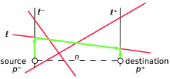
Consider the set of lines $\ell$ which intersect both $\ell^{-}$ at distance at most $c\sqrt{n}$ from $p^{-}$ and $\ell^{+}$ at distance at most $c\sqrt{n}$ from $p^{+}$. Classic stochastic geometry arguments [based on inclusion–exclusion and a special case of the “Buffon–Sylvester problem”; see, e.g., Ambartzumian (1990)] then show that the invariant measure of this line set is given by half the difference between the summed length of the two diagonal lines minus the summed length of the two vertical lines in Figure 2.

Figure 2: Illustration of a classic stochastic geometry construction for calculating the invariant measure of the set of lines hitting both of the two vertical line segments $\ell^{\pm}$ marked out by the two horizontal lines.

Hence, the probability of no unconditioned Poisson lines falling in this set is

$$\exp\bigl{(}-\tfrac{1}{2}\bigl{(}2\sqrt{4c^{2}n+n^{2}}-2n\bigr{)}\bigr{)}\geq\exp(-2c^{2}),$$

and, as a consequence, the resulting mean excess is bounded below by

$$\sqrt{n}\int_{0}^{\infty}e^{-2c^{2}}\,{d}c=\frac{1}{2}\sqrt{\frac{\pi n}{2}},$$

attributable to the parts of the route which lie on the conditioned lines $\ell^{-}$, $\ell^{+}$. (Excess along the unconditioned line $\ell$ itself is bounded above by $\sqrt{4c^{2}n+n^{2}}-n\leq 2c^{2}$ and is hence negligible in the case of large $n$.)

This rather trivial example makes it clear that being permitted to use more than one line (in addition to the two conditioned lines) will reduce the excess principally by rounding off the corners at the start and finish of the journey. Thus, it is clear [as is indeed apparent from details of the computations in Aldous and Kendall (2008), Theorem 3] that the logarithmic excess in the full construction is a cost which arises entirely from the business of getting on and off an efficient route between source and destination.

1.2 Making connections

Any two specified points $p^{-}$ and $p^{+}$ in the plane will almost surely not be hit by any of the lines of a given isotropic stationary Poisson line process $\Pi$ and will therefore fail to be connected by $\Pi$. Accordingly, we establish the convention that movement from $p^{-}$ to $p^{+}$ occurs as follows: first, use the Poisson tessellation to construct the cell $\mathcal{C}(p^{-},p^{+})$ containing $p^{-}$ and $p^{+}$ which arises by deleting all Poisson lines which separate $p^{-}$ from $p^{+}$. Now, proceed from the source $p^{-}$ in exactly the opposite direction to that of $p^{+}$ until one first encounters a Poisson line [which will be part of the cell boundary $\partial\mathcal{C}(p^{-},p^{+})$]. Then, continue along the line in one or the other direction, clockwise or counterclockwise, proceeding along the boundary of the cell $\mathcal{C}(p^{-},p^{+})$. Continue until one reaches the ray extending from $p^{-}$ and through $p^{+}$. Then, proceed down this ray to the destination $p^{+}$ (Figure 3). Thus, we consider near-geodesics; routes based on semiperimeters of the cell $\mathcal{C}(p^{-},p^{+})$. These are to be considered in contrast to network geodesics, which always use the shortest network path and can therefore be found only by solving a difficult optimization problem.

Figure 3: The path marked by arrows illustrates one of the two possible journeys around the cell $\mathcal{C}(p^{-},p^{+})$ which start at source $p^{-}$ and end at destination $p^{+}$.

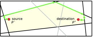
Evidently, this is a conservative option for plumbing nodes into the Poisson network produced by $\Pi$, suitable if we wish to produce upper bounds on connection lengths and adopted without further comment in what follows. We suppose the choice of whether to travel clockwise or counterclockwise around the cell $\mathcal{C}(p^{-},p^{+})$ (or, equivalently, which semiperimeter to choose) is made at random and equiprobably, independently for each pair of nodes $p^{-}$, $p^{+}$. (As mentioned in Section 5, interesting and hard problems arise if the choice of route for a specific pair is influenced by the flow in the entire network.)

In contrast to true network geodesic connections, these routes can be viewed as outputs from an unsophisticated but direct semiperimeter algorithm: if one is on a Poisson line and encounters another Poisson line, then one chooses (from the three onward paths) that path which leads closest to the eventual destination without separating source from destination. This focuses attention on the Poissonian city, a region connected by routes based on a fixed stationary isotropic Poisson line process and following the above convention so as to ensure that the line process actually connects nodes. Questions addressed in Section 2 of this paper, filling in and extending the results announced in Kendall (2008), include the following:

1. What can one say about the basic geometry of these routes? Computations from Aldous and Kendall [(2008), Theorem 3] yield $\frac{4}{3}\log\operatorname{dist}(p^{-},p^{+})$ as asymptotic mean excess length as $\operatorname{dist}(p^{-},p^{+})$ tends to infinity. This can be viewed as a quantitative development of the announcement by Davidson [(1974), Theorem 5(ii)], but by how much does the traveled path deviate laterally from the Euclidean connection, and at what point is that lateral deviation greatest? (See Theorem 1.)

2. What is the order of random variation of the route lengths? (See Theorem 3.)

3. What might be said about how actual network geodesics differ from these routes? (This is discussed in Section 2.3.)

4. Finally, might actual network geodesics produce substantially smaller mean excess lengths? (Theorem 4 shows that the mean excess of true network geodesics is comparable to the mean excess of semiperimeter paths.)

1.3 Traffic flow

Given a Poissonian city, it is natural to consider traffic flow. Suppose, for example, that the city is represented by $\operatorname{ball}(\mathbf{o},n)$, a disc centered at $\mathbf{o}$ and of radius $n$, connected by roads provided by a stationary isotropic Poisson line process $\Pi$. Suppose that each pair of points $p^{-}$ and $p^{+}$ in the disc generates a constant infinitesimal amount of traffic ${d}p^{-}\,{d}p^{+}$, divided equally between each of the two connecting routes generated according to the semiperimeter algorithm described above. Suppose further that we condition on the event of a Poisson line passing through the center $\mathbf{o}$ of the disc. Let

$$\mathcal{D}_{n}=\{(p^{-},p^{+})\in\operatorname{ball}(\mathbf{o},n)^{2}\dvtx p^{-}_{1}<p^{+}_{1},\mathbf{o}\in\partial\mathcal{C}(p^{-},p^{+})\}$$ (1)

denote the region in $4$-space corresponding to $p^{-}$, $p^{+}$ in $\operatorname{ball}(\mathbf{o},n)$ for which $p^{-}$ lies to the left of $p^{+}$ (imposed by the inequality $p^{-}_{1}<p^{+}_{1}$, where $p^{-}_{1}$, $p^{+}_{1}$ are the $x$-coordinates of source and destination nodes) and one of the two possible routes passes through $\mathbf{o}$.

Questions addressed in Section 3 include:

1. What is the dependence on $n$ of the mean $\mathbb{E}[T_{n}]$ of

   $$T_{n} = \frac{1}{2}\int\!\!\int\mathbb{I}_{[(p^{-},p^{+})\in\mathcal{D}_{n}]}\,{d}p^{-}\,{d}p^{+}$$

   $$= \frac{1}{2}\int\!\!\int_{\operatorname{ball}(\mathbf{o},n)^{2}}\mathbb{I}_{[p^{-}_{1}<p^{+}_{1},\mathbf{o}\in\partial\mathcal{C}(p^{-},p^{+})]}\,{d}p^{-}\,{d}p^{+},$$

   the total amount of traffic passing through the center $\mathbf{o}$? This quantity scales as $n^{3}$, following from scaling arguments using basic stochastic geometry. However, one can in fact compute the constant of asymptotic proportionality (Theorem 5).

2. Indeed, Aldous has asked whether the scaled flows $T_{n}/n^{3}$ have a nondegenerate limiting distribution. (The answer is that they do: see Theorem 7 and Corollary 9.)

3. Does uniform integrability hold for the sequence of $T_{n}/n^{3}$ as $n\to\infty$? If not, then there might exist a well behaved limiting distribution, but the mean of $T_{n}/n^{3}$ might converge to a higher value than that of the limit. Were this the case, it could be viewed as a kind of stochastic congestion result. (The results of Theorem 5 and Lemma 8 indicate why uniform integrability does hold; it is possible to push this further, as indicated in Section 3.4.)

Section 4 provides a comparison by giving an overview of analogous results for flows in cities built on grids (Manhattan cities). The concluding Section 5 adds some further remarks and mentions possible future research directions.

1.4 Directory of results

Finally, we present a directory of the main results so as to assist the reader in navigating around this paper.

In Section 1.2, Theorem 1 establishes statistical asymptotics for the maximum lateral deviation of a near-geodesic from the corresponding Euclidean path; asymptotically, the maximum will be located uniformly along the path, with extent given by the radial part of a four-dimensional Gaussian vector with variance which is quadratic in the location of the maximum and which vanishes at the two endpoints. A preliminary Lemma 2 then leads to Theorem 3, which produces an asymptotic bound $\frac{20}{27}\log n$ for the variance of the excess of near-geodesic length over Euclidean path length, for a near-geodesic started at a point and going off to a line at distance $n$ from the point. Theorem 4 generates an asymptotic lower bound $2(\log 4-\frac{5}{4})\log n$ on the mean excess for any path between two fixed points separated by distance $n$. The numerical value $0.27258872\ldots$ of the constant of proportionality here should be compared with the corresponding constant $\frac{4}{3}=1.33\ldots$ for near-geodesics [Aldous and Kendall (2008)].

In Section 3 the focus changes to flows in networks built from Poisson line processes. After introducing the notion of a “Poissonian city” (based on a disc of radius $n$), Theorem 5 shows that the traffic flow $T_{n}$ through the center has asymptotic mean $2n^{3}$. Corollary 6 reports a refinement of the detailed asymptotics; Theorem 7 (supported by Lemma 8) establishes the existence of a limiting distribution for $T_{n}/n^{3}$—although the result only gives a geometric characterization—and Corollary 9 confirms that this limit distribution is nondegenerate.

2 Making connections in the Poissonian city

Asymptotic arguments applied to formulas from stochastic geometry indicate both the geometry of the routes provided by the unsophisticated semiperimeter algorithm described above (including the extent of random variation in length) and also ways in which they differ from true network geodesics between source and destination nodes. We begin by discussing the asymptotic distribution of the location and extent of the maximum lateral displacement of a semiperimeter route from the corresponding Euclidean geodesic.

2.1 Maximum lateral displacement

Consider the height and location of the maximum lateral displacement of one of the $\partial\mathcal{C}(p^{-},p^{+})$ semiperimeter routes from a source $p^{-}$ to a destination $p^{+}$. Figure 4

Figure 4: A plot of $1000$ semiperimeters of cells $\partial\mathcal{C}(p^{-},p^{+})$ based on a distance $n=\operatorname{dist}(p^{-}$, $p^{+})=1000$. The dots indicate the maximum lateral displacements from the horizontal axis between source and destination. The figure has been subjected to vertical exaggeration by a factor of $\sqrt{n}/4$.

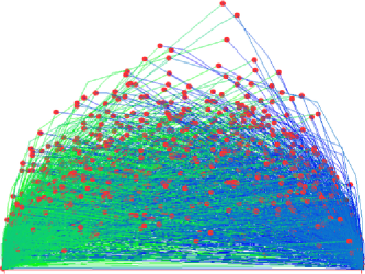
illustrates $1000$ realizations of such routes, with maxima marked by discs, when source and destination are separated by distance $n=1000$. Such simulations suggest the existence of a limiting distribution under scaling for the extent and location of the maximum lateral displacement, and stochastic geometry arguments show that this is indeed the case.

Theorem 1

Consider two points $p^{-}=\mathbf{o}=(0,0)$ and $p^{+}=(n,0)$ located along the $x$-axis and also a path between these points based on $\partial\mathcal{C}(p^{-},p^{+})\cap\{(x,y)\dvtx y\geq 0\}$. Locate the maximum lateral displacement of $\partial\mathcal{C}(p^{-},p^{+})\cap\{(x,y)\dvtx y\geq 0\}$ from the $x$-axis (and thus from the Euclidean geodesic between $p^{-}$ and $p^{+}$) at $(nU_{n},\sqrt{n}V_{n})$. The joint distribution of $(U_{n},V_{n})$ then has the following weak limit $(U,V)$ as $n\to\infty$:

1. [(a)]

2. the scaled location $U$ is uniformly distributed over $[0,1]$;

3. conditional on $U=u\in(0,1)$, the scaled displacement $V$ is distributed as the length of a four-dimensional Gaussian vector with variance $2u(1-u)$.

Let $p^{-}$, $p^{+}$ be located at $\mathbf{o}$ and $(n,0)$ on the $x$-axis and let the maximum displacement be located at $(nU_{n},\sqrt{n}V_{n})$, as in the statement of the theorem, so that

$$\sqrt{n}V_{n} = \max\{y\dvtx(x,y)\in\partial\mathcal{C}(p^{-},p^{+})\},$$

$$\bigl{(}nU_{n},\sqrt{n}V_{n}\bigr{)} \in \partial\mathcal{C}(p^{-},p^{+}).$$

(Almost sure uniqueness of $U_{n}$ is a consequence of the fact that a stationary isotropic Poisson line process almost surely contains no horizontal lines.)

The proof is a variation on ideas in the proof of Theorem 3 in Aldous and Kendall (2008). Consider the point process formed by intersections of lines $\ell^{-}$, $\ell^{+}$ from $\Pi$, subject to the following, additional, requirements:

1. no further lines from $\Pi$ separate the intersection $\ell^{-}\cap\ell^{+}$ from the segment of length $n$ formed between the pair of points $p^{-}=\mathbf{o}$, $p^{+}=(n,0)$;

2. one of the intersecting lines $\ell^{-}$ has positive slope, the other $\ell^{+}$ has negative slope and neither line intersects the segment formed between the pair of points $p^{-}$, $p^{+}$.

Topological arguments show that there must be just two points in this point process, one above and one below the $x$-axis, and the point above the $x$-axis must be located at $(nU_{n},\sqrt{n}V_{n})$. The intensity of the point process in the upper half-plane is given by

$$\rho(x,y) = \tfrac{1}{4}\bigl{(}\sin\alpha+\sin\beta-\sin(\alpha+\beta)\bigr{)}$$

$${}\times\exp\bigl{(}-\tfrac{1}{2}\bigl{(}\sqrt{x^{2}+y^{2}}+\sqrt{(n-x)^{2}+y^{2}}-n\bigr{)}\bigr{)},$$

where $\alpha$, $\beta\in(0,\pi)$ are the interior angles at $\mathbf{o}$ and $(n,0)$ of the triangle formed by $(x,y)$ and these two points. Here, the exponential factor is contributed by requirement 1 above, since Slivynak’s theorem can be used to show that the unit intensity stationary isotropic Poisson property is preserved by conditioning on two lines from $\Pi$ intersecting at $(x,y)$ and then removing those two lines. Employing the fact that the intensity of the point process formed by intersections of lines from the unit intensity line process $\Pi$ is $\frac{\pi}{2}$, requirement 2 can be shown to lead to the factor

$$\frac{\pi}{2}\times\frac{1}{\pi}\int_{0}^{\alpha}\int_{0}^{\beta}\frac{1}{2}\sin(\theta+\psi)\,{d}\psi\,{d}\theta$$

$$\qquad=\frac{1}{4}\bigl{(}\sin\alpha+\sin\beta-\sin(\alpha+\beta)\bigr{)}.$$

It follows that $(U_{n},V_{n})$ has joint density on the upper half-plane given asymptotically for large $n$ when $0<u<1$ and $v>0$ by

$$n^{3/2}\rho\bigl{(}nu,\sqrt{n}v\bigr{)} = \frac{n^{3/2}}{4}\bigl{(}\sin\alpha+\sin\beta-\sin(\alpha+\beta)\bigr{)}$$

$${}\times\exp\Biggl{(}-\frac{n}{2}\Biggl{(}\sqrt{u^{2}+\frac{v^{2}}{n}}+\sqrt{(1-u)^{2}+\frac{v^{2}}{n}}-1\Biggr{)}\Biggr{)}$$

$$\sim \frac{n^{3/2}}{4}\exp\biggl{(}-\frac{1}{4}\frac{v^{2}}{u(1-u)}\biggr{)}$$

$${}\times\bigl{(}\sin(\alpha)\bigl{(}1-\cos(\beta)\bigr{)}+\sin(\beta)\bigl{(}1-\cos(\alpha)\bigr{)}\bigr{)}.$$

Converting the sines and cosines to expressions in $u$ and $v$, as $n\to\infty$

$$\frac{n^{3/2}}{4}\rho\bigl{(}nu,\sqrt{n}v\bigr{)}$$

$$\qquad\sim\frac{n^{3/2}}{4}\exp\biggl{(}-\frac{1}{4}\frac{v^{2}}{u(1-u)}\biggr{)}$$

$$\qquad\quad{}\times\biggl{(}\frac{{v}/{\sqrt{n}}}{\sqrt{u^{2}+{v^{2}}/{n}}}\biggl{(}1-\frac{1-u}{\sqrt{(1-u)^{2}+{v^{2}}/{n}}}\biggr{)}$$

$$\qquad\quad\hskip 17.8pt{}+\frac{{v}/{\sqrt{n}}}{\sqrt{(1-u)^{2}+{v^{2}}/{n}}}\biggl{(}1-\frac{u}{\sqrt{u^{2}+{v^{2}}/{n}}}\biggr{)}\biggr{)}$$

$$\qquad\to\frac{1}{8}\frac{v^{3}}{u^{2}(1-u)^{2}}\exp\biggl{(}-\frac{1}{4}\frac{v^{2}}{u(1-u)}\biggr{)}.$$

This can be identified as the joint density corresponding to the limiting distribution of $U_{n}$ and $V_{n}$ given in the theorem; weak convergence follows from Fatou’s lemma.

Simulation studies (from which Figure 4 was derived) confirm these asymptotics.

2.2 Random variation via growth processes

The direct stochastic geometry method is highly effective for computing detailed asymptotics of mean-value quantities but leads to burdensome calculations for second order quantities such as variances. We therefore turn to an alternate approach based on random growth processes. The maximum analyzed in Section 2.1 occurs at the point of intersection of the trajectories of two independent growth processes, together representing the lateral deviation of the path from the Euclidean geodesic between source and destination nodes. One growth process is viewed as starting from the source node $p^{-}$ and one from the destination node $p^{+}$, tracing out the relevant semiperimeter of $\mathcal{C}(p^{-},p^{+})$ by describing the height as a function of arc length along the semiperimeter. The two processes $\{H^{\pm}_{s}\dvtx s\geq 0\}$ are given by heights $H^{\pm}_{s}$ above the $y$-axis at arc length distance $s$ along the respective path from the originating node ($p^{-}$ for $H^{+}$, $p^{+}$ for $H^{-}$). Let $\Theta^{\pm}_{s}$ be the angle made by the path with the $x$-axis, where the angle measurement is oriented depending on the label “$\pm$” so that $\Theta^{\pm}_{0}=\pi$ (since the path commences by setting out in the opposite direction to that of its goal). Then, $\frac{{d}}{{d}s}H^{\pm}_{s}=\sin\Theta^{\pm}_{s}$ [except for isolated points at which the slope of $\partial\mathcal{C}(p^{-},p^{+})$ changes]. Changes in $\Theta^{\pm}$ occur when the path is intercepted by a line from $\Pi$ which also intersects that part of the $x$-axis with $p^{\mp}$ deleted which does not contain $p^{\pm}$. Indeed, starting at arc length $s$ along the path from $p^{\mp}$, the angle $\Theta^{\pm}$ remains constant for an Exponentially distributed length of rate $\frac{1}{2}(1-\cos\Theta^{\pm}_{s})$, after which the angle jumps to a lower value $\Theta^{\pm}_{s-}+\Delta\Theta^{\pm}_{s}<\Theta^{\pm}_{s-}$. The hitting properties of Poisson line processes can be used to show

$$\mathbb{P}[-\Delta\Theta^{\pm}_{s}\leq\phi|\Theta^{\pm}_{s-}=\theta]=\frac{1-\cos\phi}{1-\cos\theta}\qquad\mbox{where }0\leq\phi\leq\theta.$$ (3)

(Jump processes such as $\Theta$ are taken to be càdlàg so that $\lim_{s\searrow t}\Theta_{s}=\Theta_{t}$, and we write $\Theta_{-}$ for the process of left limits.) We suppose the growth processes $H^{\pm}$ evolve for all time according to the dynamics described above. Let $X^{\pm}_{s}$ be the distance from $p^{\mp}$ when resolved along the axis from source $p^{\mp}$ to destination $p^{\pm}$, so $\frac{{d}}{{d}s}X^{\pm}_{s}=\sec\Theta^{\pm}_{s}$ (except for isolated points of discontinuity of $\Theta$).

Figure 5: Illustration of $H^{+}$ construction. The growth process $H^{+}_{s}$ tracks height as a function of arc length $s$. The angle of slope $\Theta^{+}_{s}$ is an auxiliary process governed by a Poisson stochastic differential equation, jumping when the path is intercepted by a line from $\Pi$ which also intersects the negative $x$-axis.

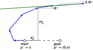
Figure 5 illustrates the $H^{+}$ construction.

Analysis of growth process using Lévy processes

For the sake of clarity of exposition, we now drop the superscripted $\pm$.

It is convenient to apply a random time change $t=s-X_{s}$ using the excess of arc length over distance traveled toward the goal; in the new time scale, the angle $\Theta$ changes according to a Poisson process of incidents of rate $\frac{1}{2}$ while $\frac{{d}H}{{d}t}=\sin\Theta/(1-\cos\Theta)$, $\frac{{d}X}{{d}t}=\cos\Theta/(1-\cos\Theta)$. This gives a stochastic differential equation for $H$ and $X$, driven indirectly by a half-unit rate Poisson counting process $N$ via the auxiliary process $\Theta$:

$${d}H = \frac{\sin\Theta}{1-\cos\Theta}\,{d}t;$$

$${d}X = \frac{\cos\Theta}{1-\cos\Theta}\,{d}t;$$ (4)

$${d}\Theta = \Delta\Theta\,{d}N.$$

The distribution of the jump $\Delta\Theta$ is given by (3), and the jump $\Delta\Theta$ at a jump of $N$ is conditionally independent of the past given $\Theta_{-}$ at that time. Note that (2.2) can be viewed as driven by a marked Poisson process, obtained by marking the incidents of $N$ by the jumps of $\Theta$, with mark distribution (conditional on the left limit $\Theta_{-}$) given by (3). Using this terminology and approach, we will now show that the excess $\sigma(n)=\inf\{t\dvtx X_{t}\geq n\}=\inf\{t\dvtx\int_{0}^{t}\frac{\cos\Theta_{u}}{1-\cos\Theta_{u}}\,{d}u\geq n\}$ at given distance $X=n$ has standard deviation asymptotically proportional to $\sqrt{\log n}$ for large $n$.

Figure 6: Illustration of initial segment of a path used to provide an upper bound on the excess acquired before $X=0$. This initial segment is made up of three line segments, of lengths $T_{1}$, $T_{2}$, and finally a length bounded above by $T_{1}\sec U$. Here, $T_{1}$, $T_{2}$, $U$ are independent with distributions as given in the text.

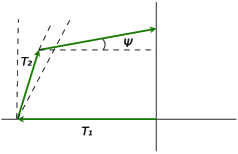
To establish this result it is simplest to consider the growth process begun with $X_{0}=0$ and $\Theta_{0}$ lying in the range $(0,\pi/2]$. We must therefore control the amount of excess required to achieve this over the initial segment of the path. Since $X=0$ at both ends of this segment, this excess can be bounded above by the length of the initial segment of the path indicated in Figure 6. This path uses the following directions until it first hits the $y$-axis: it first runs along the negative $x$-axis until it encounters a line of angle between $\frac{\pi}{3}$ and $\frac{\pi}{2}$; it then moves upward along this line until it encounters a line of angle between $0$ and $\frac{\pi}{3}$, then along that line. The first segment is of length $T_{1}$, Exponentially distributed of rate $\frac{1}{4}$. The second segment is of length stochastically bounded above by $T_{2}$, Exponentially distributed of rate $\frac{1}{4}$. The final segment is of length stochastically bounded above by $T_{1}\sec U$, where $U$ has density $\frac{2}{\sqrt{3}}\cos u$ for $0<u<\frac{\pi}{3}$ (this uses a stochastic monotonicity argument applied to the conditional distribution of the angle of the third line segment given the angle of the second line segment). We may take $T_{1}$, $T_{2}$, $U$ to be independent.

The quantity $T_{1}+T_{2}+T_{1}\sec U$ is an upper bound on the path length of the initial segment and has finite mean given by $8(1+\frac{\pi}{3\sqrt{3}})$ and finite second moment given by $32(3+\frac{2}{\sqrt{3}}(\pi+\log(2+\sqrt{3})))$. It follows that the contribution of the actual initial segment to the mean and variance of the excess is bounded and may be ignored if we can establish logarithmic increase in variance of the remainder. Accordingly, we may suppose our growth process begins with $X_{0}=0$ and with $\Theta_{0}$ lying between $0$ and $\frac{\pi}{2}$, distributed according to the density $\cos\theta$ for $0<\theta<\frac{\pi}{2}$. [This is because the growth process will intersect the positive $y$-axis in the first intercept which makes an angle with the horizontal in the range $(0,\frac{\pi}{2})$.]

We now address the question of the variance of $\sigma(n)$ (based on $X_{0}=0$) in three stages. First, we use trigonometry and probabilistic coupling to relate the negative log angle $-\log\Theta$ to a Lev́y subordinator $\xi$. We then state and prove a lemma on analogous mean and variance asymptotics for $\tau(n)=\inf\{t\dvtx\int_{0}^{t}\exp(2\xi_{u})\,{d}u\geq n\}$. Finally, we state and prove a theorem which uses approximations and coupling to establish the required mean and variance asymptotics for $\sigma(n)$.

For the first stage, note that if $0\leq\Theta\leq\frac{\pi}{2}$, then, by trigonometry and calculus, we can convert the first two partial sums of the Laurent series for $\frac{\cos\Theta}{1-\cos\Theta}$ into upper and lower bounds over $[0,\frac{\pi}{2}]$:

$$\frac{2}{\Theta^{2}}-\frac{5}{6}\leq\frac{\cos\Theta}{1-\cos\Theta}\leq\frac{2}{\Theta^{2}}.$$ (5)

The application of the distributional information in (3) to a jump $\Delta\Theta=\Theta-\Theta_{-}$ produces a unit Exponential random variable:

$$\mathcal{J}=-\log\biggl{(}\frac{1-\cos(-\Delta\Theta)}{1-\cos\Theta_{-}}\biggr{)}.$$ (6)

We can thus mark independently each jump of the Poisson process $N$ using the unit Exponential mark distribution of $\mathcal{J}$. The mark $\mathcal{J}$ can be used, together with $\Theta_{-}$, to reconstruct the actual jump of $\Theta$, using (6). Bearing in mind that $\Delta\Theta<0$, we may write

$$\mathcal{J}=f(\log\Theta_{-})-f(\log(-\Delta\Theta)),$$

where $f(x)=\log(1-\cos e^{x})$. Calculus shows that $f^{\prime}>0$ and $f^{\prime\prime}<0$ over the range $(-\infty,\log\frac{\pi}{2})$. Hence, if $x\leq\log\Theta_{-}\leq\log\frac{\pi}{2}$, then

$$\frac{\pi}{2}\leq f^{\prime}(\log\Theta_{-})\leq f^{\prime}(x)=\frac{e^{x}\sin e^{x}}{1-\cos e^{x}}<2=\lim_{x\to-\infty}\frac{e^{x}\sin e^{x}}{1-\cos e^{x}}.$$

However, $0<-\Delta\Theta<\Theta_{-}$ and $\mathcal{J}=\int_{\log(-\Delta\Theta)}^{\log\Theta_{-}}f^{\prime}(x)\,{d}x$; therefore,

$$f^{\prime}(\log\Theta_{-})\bigl{(}\log\Theta_{-}-\log(-\Delta\Theta)\bigr{)}\leq\mathcal{J}\leq 2\bigl{(}\log\Theta_{-}-\log(-\Delta\Theta)\bigr{)}.$$

Hence, for $0<-\Delta\Theta<\Theta_{-}\leq\frac{\pi}{2}$,

$$-\log\biggl{(}1-\exp\biggl{(}-\frac{2}{\pi}\mathcal{J}\biggr{)}\biggr{)} \leq -\log\biggl{(}1-\exp\biggl{(}-\frac{\mathcal{J}}{f^{\prime}(\log\Theta_{-})}\biggr{)}\biggr{)}$$

$$\leq -\log\biggl{(}\frac{\Theta_{-}+\Delta\Theta}{\Theta_{-}}\biggr{)}=-\Delta\log\Theta$$

$$\leq -\log\biggl{(}1-\exp\biggl{(}-\frac{1}{2}\mathcal{J}\biggr{)}\biggr{)}.$$

For future reference, note that $-\log(1-\exp(-\frac{1}{2}\mathcal{J}))$ is distributed as the maximum $T^{\prime}\vee T^{\prime\prime}$ of two independent unit-mean Exponential random variables $T^{\prime}$ and $T^{\prime\prime}$, and, in particular, it has mean $\frac{3}{2}$ and variance $\frac{5}{4}$. On the other hand $-\log(1-\exp(-\frac{2}{\pi}\mathcal{J}))$ has probability density $\frac{\pi}{2}(1-e^{-x})^{{\pi}/{2}-1}e^{-x}$ for $x>0$, and the square of its negative exponential $(1-\exp(-\frac{2}{\pi}\mathcal{J}))^{2}$ (which will play a role later on) has probability density

$$\frac{\pi}{4}\bigl{(}1-\sqrt{x}\bigr{)}^{{\pi}/{2}-1}\frac{1}{\sqrt{x}}\qquad\mbox{for }0<x<1.$$ (8)

Thus, a coupling construction indicated by the inequalities of (2.2) permits approximation of the negative logarithm of the angle process by $\eta\leq-\log(\Theta/\Theta_{0})\leq\xi$. Here, $\eta$, $\xi$ are nondecreasing pure-jump Lévy processes (hence subordinators) which have jumps at the same times as those of $-\log\Theta$ (namely, at incidents of the Poisson counting process $N$ of intensity $\frac{1}{2}$), but with jump distributions given by the distributions of $-\log(1-\exp(-\frac{2}{\pi}\mathcal{J}))$ and $-\log(1-\exp(-\mathcal{J}/2))$, respectively. For future reference, note also that the Laplace exponent $\Phi(q)=-\frac{1}{t}\log\mathbb{E}[e^{-q\xi_{t}}]$ of $\xi$ can be computed as $\Phi(q)=\frac{q(3+q)}{2(1+q)(2+q)}$ for $q>-1$, while $M_{s}=\xi_{s}-\frac{3}{4}s$ defines a martingale, as does $M^{2}_{s}-\frac{5}{8}s$. In particular, $M$ is an $L^{2}$-martingale.

The discrepancy between coupled jumps of $\xi$ and $-\log\Theta$ can be controlled by

$$0\leq\Delta\xi-\biggl{(}-\log\frac{\Theta_{-}+\Delta\Theta}{\Theta_{-}}\biggr{)}\leq\log\biggl{(}\frac{1-\exp(-\mathcal{J}/f^{\prime}(\log\Theta_{-}))}{1-\exp(-{\mathcal{J}}/{2})}\biggr{)}.$$ (9)

Now, if $0\leq a\leq\frac{\pi}{2}$, then we can use the inequalities $\sin\frac{a}{2}\leq\frac{a}{2}$, $\cos^{2}\frac{a}{2}\geq\frac{1}{2}$ and the convexity of $\tan^{2}\frac{a}{2}$ over this range to establish the simple bound

$$\frac{1}{f^{\prime}(\log a)}=\frac{1-\cos a}{a\sin a}\leq\frac{1-\cos a}{\sin^{2}a}=\frac{1}{2}+\frac{\tan^{2}({a}/{2})}{2}\leq\frac{1}{2}+\frac{a^{2}}{4}$$

and so (using $\Theta\leq\frac{\pi}{2}$ to apply the above inequality)

$$\log\biggl{(}\frac{1-\exp(-\mathcal{J}/f^{\prime}(\log\Theta_{-}))}{1-\exp(-{\mathcal{J}}/{2})}\biggr{)} \leq \log\biggl{(}1+\frac{1-\exp(-({\Theta_{-}^{2}}/{2})({\mathcal{J}}/{2}))}{\exp({\mathcal{J}}/{2})-1}\biggr{)}$$

$$\leq \log\biggl{(}1+\frac{{\mathcal{J}}/{2}}{\exp({\mathcal{J}}/{2})-1}\frac{\Theta_{-}^{2}}{2}\biggr{)}$$

$$\leq \frac{{\mathcal{J}}/{2}}{\exp({\mathcal{J}}/{2})-1}\frac{\Theta_{-}^{2}}{2}\leq\frac{\Theta_{-}^{2}}{2}$$

$$\leq \frac{1}{2}\exp(-2\eta_{-}).$$

Applying this upper bound on the jumps, it follows that we can control the total discrepancy between $\xi$ and $-\log\Theta$ by

$$0\leq\xi_{t}-\bigl{(}-\log(\Theta_{t}/\Theta_{0})\bigr{)}\leq\frac{1}{2}\mathop{\sum_{w\leq t:}}_{\Delta N_{w}>0}\exp(-2\eta_{w-}).$$ (10)

However, the right-hand side is increasing in $t$ and has a limit which can be expressed in terms of a simple perpetuity. Indeed,

$$\sum_{w\dvtx\Delta N_{w}>0}\exp(-2\eta_{w-})=U_{t}\leq U_{\infty}=\Biggl{(}1+\sum_{k=1}^{\infty}\prod_{m=1}^{k}\exp(-2\Delta_{m}\eta)\Biggr{)},$$

where $\Delta_{m}\eta$ is the $m$th jump of $\eta$. A classical calculation gives the first and second moments of the perpetuity final value $U_{\infty}$ in terms of first and second moments of $\exp(-2\Delta_{m}\eta)$ [see, e.g., Vervaat (1979), Theorem 5.1]. However, we will require control of exponential moments $\mathbb{E}[\exp(zU_{\infty})]$ for positive $z$. Alsmeyer, Iksanov and Rœsler (2009) and Kellerer (1992) give results for the general case, but in our particular case the perpetuity multiplier $\exp(-2\Delta_{m}\eta)$ is positive and bounded above by $1$; moreover, its probability density (8) is bounded above near $1$, and it thus follows from monotonicity and the methods of Goldie and Grübel [(1996), Theorem 3.1] that $\mathbb{E}[\exp(zU_{\infty})]<\infty$ for all positive $z$. [In fact, the upper bound requirement on the probability density can be replaced by comparability with a Beta density; see Hitczenko and Wesołowski (2009), Section 4.]

We can now improve (5) to provide bounds in terms of Lévy subordinators:

$$\frac{2}{\Theta_{0}^{2}}\exp(2\xi-U_{\infty})-\frac{5}{6} \leq \frac{2}{\Theta^{2}}-\frac{5}{6}\leq\frac{\cos\Theta}{1-\cos\Theta}$$

$$\leq \frac{2}{\Theta^{2}}\leq\frac{2}{\Theta_{0}^{2}}\exp(2\xi).$$

Accordingly, we first establish the following lemma, which delivers the desired results for $\int\exp(2\xi_{s})\,{d}s$ rather than $X$.

Lemma 2

Define $\tau(n)$ in terms of $\int\exp(2\xi_{s})\,{d}s$ by

$$n=\int_{0}^{\tau(n)}\exp(2\xi_{s})\,{d}s.$$

Then,

$$\tau(n)=\frac{2}{3}\biggl{(}\log n-2M_{\tau(n)}+\log\biggl{(}\exp\biggl{(}\frac{2\xi_{\tau(n)}}{n}\biggr{)}\biggr{)}\biggr{)}$$ (12)

with the following asymptotics for mean and variance as $n\to\infty$:

$$\mathbb{E}[\tau(n)] = \tfrac{2}{3}\log n+O(1);$$ (13)

$$\operatorname{Var}[\tau(n)] = \tfrac{20}{27}\log n+O\bigl{(}\sqrt{\log n}\bigr{)}.$$ (14)

First note the following trivial bound for $\tau(n)$ which establishes the finiteness of $\mathbb{E}[\tau(n)]$:

$$n=\int_{0}^{\tau(n)}\exp(2\xi_{s})\,{d}s\geq\tau(n).$$

The representation (12) was motivated by heuristic time-reversal arguments and is essentially tautologous: write

$$\exp\biggl{(}2M_{\tau(n)}+\frac{3}{2}\tau(n)\biggr{)}=\exp\bigl{(}2\xi_{\tau(n)}\bigr{)}=n\times\frac{\exp(2\xi_{\tau(n)})}{n},$$

take logs and reexpress in terms of $\tau(n)$. Taking expectations, we then obtain

$$\mathbb{E}[\tau(n)]=\frac{2}{3}\biggl{(}\log n+\mathbb{E}\biggl{[}\log\biggl{(}\frac{\exp(2\xi_{\tau(n)})}{n}\biggr{)}\biggr{]}\biggr{)};$$ (15)

the expectation $\mathbb{E}[M_{\tau(n)}]$ vanishes because $\tau(n)$ has finite expectation and so the stopped martingale $M_{s\wedge\tau(n)}$ is $L^{2}$-bounded by $\mathbb{E}[M_{\tau(n)}^{2}]\leq\frac{5}{8}\mathbb{E}[\tau(n)]$.

Consider the variance of $\tau(n)-\frac{2}{3}\log(\frac{\exp(2\xi_{\tau(n)})}{n})$. Using $L^{2}$-martingale theory we find that

$$\operatorname{Var}\biggl{[}\tau(n)-\frac{2}{3}\log\biggl{(}\frac{\exp(2\xi_{\tau(n)})}{n}\biggr{)}\biggr{]}=4\biggl{(}\frac{2}{3}\biggr{)}^{2}\operatorname{Var}\bigl{[}M_{\tau(n)}\bigr{]}=\frac{16}{9}\times\frac{5}{8}\mathbb{E}[\tau(n)].$$ (16)

A uniform bound on the second moment of $\log(\frac{\exp(2\xi_{\tau(n)})}{n})$ will therefore permit us to deduce (13) and (14) from (15) and (16), and so complete the proof.

To this end, note that $Z_{n}=\exp(2\xi_{\tau(n)})$ constitutes a Lamperti transformation [Lamperti (1972)] of the subordinator $2\xi$ and therefore defines a self-similar Markov process $Z$. Using the scaling property for $Z$ and maximizing $z(\log z)^{2}$ for $0<z<1$, we obtain

$$\mathbb{E}\biggl{[}\biggl{(}\log\frac{\exp(2\xi_{\tau(n)})}{n}\biggr{)}^{2};\frac{\exp(2\xi_{\tau(n)})}{n}<1\biggr{]} = \mathbb{E}\biggl{[}(\log Z_{1})^{2};Z_{1}<1\Big{|}Z_{0}=\frac{1}{n}\biggr{]}$$

$$\leq 4e^{-2}\mathbb{E}\biggl{[}Z_{1}^{-1}\Big{|}Z_{0}=\frac{1}{n}\biggr{]}.$$

Bertoin and Yor [(2005), formula (20), drawing on Bertoin and Yor (2001)] can now be applied, together with the calculation of the Laplace exponent $\Phi(q)$ of $\xi$, to show that for $p>0$,

$$\mathbb{E}\biggl{[}Z_{1}^{-p}\Big{|}Z_{0}=\frac{1}{n}\biggr{]}=\frac{2p}{2p+1}\biggl{(}n^{p}e^{-n^{p}/2}+\biggl{(}\frac{n^{p}}{2}\biggr{)}^{1-p}\int_{0}^{n^{p}/2}v^{p-1}e^{-v}\,{d}v\biggr{)}.$$ (18)

In particular, note that each positive integral moment of $Z_{1}^{-1}$ is bounded, and, especially,

$$\mathbb{E}\biggl{[}Z_{1}^{-1}\Big{|}Z_{0}=\frac{1}{n}\biggr{]}=\frac{2}{3}\bigl{(}1+(n-1)e^{-n/2}\bigr{)}\leq\frac{2}{3}(1+2e^{-{3}/{2}}).$$

Thus, (2.2) is bounded above.

To bound $\mathbb{E}[(\log\frac{\exp(2\xi_{\tau(n)})}{n})^{2};\frac{\exp(2\xi_{\tau(n)})}{n}\geq 1]$ for $n>0$, note that $\tau(n)\leq\tau^{\prime}_{n}+1$, where $\tau^{\prime}_{n}=\inf\{t\dvtx 2\xi_{t}\geq\log n\}$. Hence,

$$\mathbb{E}\biggl{[}\biggl{(}\log\frac{\exp(2\xi_{\tau(n)})}{n}\biggr{)}^{2};\frac{\exp(2\xi_{\tau(n)})}{n}\geq 1\biggr{]}$$

$$\qquad\leq\mathbb{E}\biggl{[}(2\xi_{\tau^{\prime}_{n}+1}-\log n)^{2};\frac{\exp(2\xi_{\tau(n)})}{n}\geq 1\biggr{]}$$

$$\qquad\leq\mathbb{E}[(2\xi_{\tau^{\prime}_{n}+1}-\log n)^{2}].$$

Now, $2\xi_{\tau^{\prime}_{n}+1}-\log n$ is the independent sum of a summand of distribution $2\xi_{1}$ and a summand which is the overshoot $2\xi_{\tau^{\prime}_{n}}-\log n$. Since the jump distribution of $2\xi$ is $2(T^{\prime}\vee T^{\prime\prime})$ (for two independent unit Exponential random variables $T^{\prime}$ and $T^{\prime\prime}$), it follows by the memoryless property of the Exponential distribution that the overshoot is some mixture of the distributions of $2T^{\prime}$ and $2(T^{\prime}\vee T^{\prime\prime})$, hence stochastically dominated by $2(T^{\prime}\vee T^{\prime\prime})$. Consequently, it follows that $\mathbb{E}[(2\xi_{\tau^{\prime}_{n}+1}-\log n)^{2}]\leq\frac{111}{4}$.

Thus, $\mathbb{E}[(\log\frac{\exp(2\xi_{\tau(n)})}{n})^{2}]\leq\frac{2}{3}(1+2e^{-{3}/{2}})+\frac{111}{4}$, and hence the lemma is proved.

Note that upper bounds for $\mathbb{E}[(\log\frac{\exp(2\xi_{\tau(n)})}{n})^{2}]$ can also be obtained using the techniques of Bertoin and Yor (2002), but these bounds diverge to infinity with $n$.

We are now able to deal with the asymptotic behaviors of the mean and variance of $\sigma(n)$ as follows.

Theorem 3

With $\sigma(n)$ defined as above so that $n=X_{\sigma(n)}$ for $n>0$, for large $n$,

$$\mathbb{E}[\sigma(n)] = \tfrac{2}{3}\log n+O(1),$$ (19)

$$\operatorname{Var}[\sigma(n)] = \tfrac{20}{27}\log n+O\bigl{(}\sqrt{\log n}\bigr{)}.$$ (20)

Lemma 2 provides partial control on the asymptotic mean and variance of $\sigma(n)$ via (2.2) since $X_{t}\leq\frac{2}{\Theta^{2}_{0}}\int^{t}_{0}\exp(2\xi_{s})\,{d}s$, and so $\tau(\frac{\Theta^{2}_{0}}{2}n)\leq\sigma(n)$. By the representation (12) and integration [since $\Theta_{0}$ has density $\cos\theta$ over $(0,\frac{\pi}{2})$], we find that

$$\displaystyle\mathbb{E}\biggl{[}\tau\biggl{(}\frac{\Theta^{2}_{0}}{2}n\biggr{)}\biggr{]}=\frac{2}{3}\log n+\frac{2}{3}\mathbb{E}\biggl{[}\log\biggl{(}\frac{\Theta_{0}^{2}}{2}\biggr{)}\biggr{]}+O(1)=\frac{2}{3}\log n+O(1),$$

$$\displaystyle\operatorname{Var}\biggl{[}\tau\biggl{(}\frac{\Theta^{2}_{0}}{2}n\biggr{)}-\frac{2}{3}\log\biggl{(}\frac{\exp(2\xi_{\tau(\Theta^{2}_{0}n)})}{\Theta^{2}_{0}n}\biggr{)}\biggr{]}=\frac{20}{27}\log n+O(1).$$

The second moment of $\log(\frac{\exp(2\xi_{\tau(\Theta^{2}_{0}n)})}{\Theta^{2}_{0}n})$ being bounded, it follows that

$$\operatorname{Var}\biggl{[}\tau\biggl{(}\frac{\Theta^{2}_{0}}{2}n\biggr{)}\biggr{]}=\frac{20}{27}\log n+O\bigl{(}\sqrt{\log n}\bigr{)}.$$

We now consider the lower bounds from (2.2), delivering an upper bound for $\sigma(n)$ via

$$\int_{0}^{t}\biggl{(}\frac{2}{\Theta_{0}^{2}}\exp(2\xi_{s}-U_{s})-\frac{5}{6}\biggr{)}\,{d}s\leq\int_{0}^{t}\biggl{(}\frac{2}{\Theta_{s}^{2}}-\frac{5}{6}\biggr{)}\,{d}s\leq X_{t}.$$

First, observe what happens after the stopping time given by

$$\kappa=\biggl{(}1+\frac{5}{12}\Theta_{0}^{2}\biggr{)}\times\inf\biggl{\{}t\dvtx\frac{2}{\Theta_{t}^{2}}\geq\frac{2}{\Theta_{0}^{2}}+\frac{5}{6}\biggr{\}}.$$

We find that

$$\frac{2}{\Theta_{s+\kappa}^{2}}-\frac{5}{6} \geq \frac{2}{\Theta_{0}^{2}}\frac{\Theta_{\kappa}^{2}}{\Theta_{s+\kappa}^{2}}+\frac{5}{6}\frac{\Theta_{\kappa}^{2}}{\Theta_{s+\kappa}^{2}}-\frac{5}{6}$$

$$\geq \frac{2}{\Theta_{0}^{2}}\frac{\Theta_{\kappa}^{2}}{\Theta_{s+\kappa}^{2}}$$

and, moreover,

$$\int_{0}^{\kappa}\biggl{(}\frac{2}{\Theta_{s}^{2}}-\frac{5}{6}\biggr{)}\,{d}s\geq-\frac{5}{6}\times\frac{\kappa}{1+({5}/{12})\Theta_{0}^{2}}+\frac{({5}/{12})\Theta_{0}^{2}}{1+({5}/{12})\Theta_{0}^{2}}\times\frac{2\kappa}{\Theta_{0}^{2}}=0.$$

This will allow us to disregard the effects of the $-\frac{5}{6}$ term, so long as we can bound the second moment of $\kappa$. To this end, introduce $\zeta$, a Lévy subordinator jumping at the incidents of the underlying Poisson process $N$, with jumps coupled to those of the other processes so that $\zeta\leq\eta\leq-\log(\Theta/\Theta_{0})$, and with

$$\Delta\zeta=\mathbb{I}_{[-\log(1-\exp(-({2}/{\pi})\mathcal{J}))>1]}.$$

Since these jumps are all of sizes $0$ or $1$, we can view $\zeta$ as a Poisson counting process run at rate $\nu<\frac{1}{2}$. Moreover, since $0<\Theta_{0}\leq\frac{\pi}{2}$, we have

$$\kappa \leq \biggl{(}1+\frac{5}{12}\Theta_{0}^{2}\biggr{)}\inf\biggl{\{}t\dvtx\frac{2}{\Theta_{0}^{2}}\exp(2\zeta_{t})\geq\frac{2}{\Theta_{0}^{2}}+\frac{5}{6}\biggr{\}}$$

$$\leq \biggl{(}1+\frac{5\pi^{2}}{48}\biggr{)}\inf\biggl{\{}t\dvtx\zeta_{t}\geq\frac{1}{2}\log\biggl{(}1+\frac{5\pi^{2}}{48}\biggr{)}\biggr{\}},$$

and the boundedness of the second moment of the right-hand side of these inequalities follows directly by comparison with a Gamma random variable, derived from basic Poisson process properties. Hence, $\mathbb{E}[\kappa^{2}]<\infty$.

So, consider $\widetilde{\xi}_{s}=\xi_{\kappa+s}-\xi_{\kappa}$ and $\widetilde{\tau}(n)=\inf\{t\dvtx\int^{t}_{0}\exp(2\widetilde{\xi}_{s})\,{d}s=n\}$. We will bound $\sigma(n)$ above by a stopping time $\kappa+\widetilde{\tau}(\frac{\Theta^{2}_{0}}{2}n)+\rho$, where $\rho$ is chosen to compensate for the undershoot of $n$ at time $t=\kappa+\widetilde{\tau}(\frac{\Theta^{2}_{0}}{2}n)$ caused by the $U$ contribution in

$$\int_{0}^{t}\biggl{(}\frac{2}{\Theta_{0}^{2}}\exp(2\xi_{s}-U_{s})-\frac{5}{6}\biggr{)}\,{d}s\leq X_{t}.$$

We find

$$\int_{0}^{\kappa+\widetilde{\tau}(({\Theta^{2}_{0}}/{2})n)+\rho}\biggl{(}\frac{2}{\Theta^{2}}-\frac{5}{6}\biggr{)}\,{d}s$$

$$\qquad\geq\int_{0}^{\widetilde{\tau}(({\Theta^{2}_{0}}/{2})n)+\rho}\frac{2}{\Theta^{2}_{0}}\exp(2\widetilde{\xi}_{s}-U_{\kappa+s})\,{d}s$$

$$\qquad\geq\exp\bigl{(}-U_{\kappa+\widetilde{\tau}(({\Theta^{2}_{0}}/{2})n)}\bigr{)}\biggl{(}n+\frac{2}{\Theta^{2}_{0}}\rho\exp\bigl{(}2\widetilde{\xi}_{\widetilde{\tau}(({\Theta^{2}_{0}}/{2})n)}\bigr{)}\biggr{)}.$$

Thus, we can choose $\rho$ to compensate for the undershoot so that

$$\exp\bigl{(}-U_{\kappa+\widetilde{\tau}(({\Theta^{2}_{0}}/{2})n)}\bigr{)}\biggl{(}n+\frac{2}{\Theta^{2}_{0}}\rho\exp\bigl{(}2\widetilde{\xi}_{\widetilde{\tau}(({\Theta^{2}_{0}}/{2})n)}\bigr{)}\biggr{)}=n;$$

this is fulfilled by the choice

$$\rho=\bigl{(}\exp\bigl{(}U_{\kappa+\widetilde{\tau}(({\Theta^{2}_{0}}/{2})n)}\bigr{)}-1\bigr{)}\times\biggl{(}\frac{\exp(2\widetilde{\xi}_{\widetilde{\tau}(({\Theta^{2}_{0}}/{2})n)})}{({\Theta^{2}_{0}}/{2})n}\biggr{)}^{-1}.$$

Now, the first factor is bounded above by $\exp(U_{\infty})$, and we have already noted that $\mathbb{E}[\exp(zU_{\infty})]<\infty$ for all $z>0$ as a consequence of perpetuity theory. The second factor is distributionally a randomization over $m$ of $(\exp(2\xi_{\tau(m)})/m)^{-1}$, and we have already noted that equation (18), the Lamperti transformation and the results of Bertoin and Yor allow us to bound $\mathbb{E}[(\exp(2\xi_{\tau(m)})/m)^{-p}]$ uniformly in $m$ for any fixed $p\geq 1$. We may thus deduce $\mathbb{E}[\rho^{2}]<\infty$ as a consequence of the Cauchy–Schwarz inequality.

Accordingly, we find that

$$\sigma(n)\leq\kappa+\widetilde{\tau}\biggl{(}\frac{\Theta^{2}_{0}}{2}n\biggr{)}+\rho$$

bounds $\sigma(n)$ above by a stopping time with expectation $\frac{2}{3}\log n+O(1)$; moreover, we may apply the representation (12) to deduce that, up to terms whose second moments are $O(1)$,

$$\widetilde{\tau}\biggl{(}\frac{\Theta_{0}^{2}}{2}n\biggr{)}-\tau\biggl{(}\frac{\Theta_{0}^{2}}{2}n\biggr{)}\approx 2M_{\kappa+\widetilde{\tau}(({\Theta_{0}^{2}}/{2})n)}-2M_{\tau(({\Theta_{0}^{2}}/{2})n)},$$

which itself must be of uniformly bounded second moment:

$$\mathbb{E}\bigl{[}\bigl{(}2M_{\kappa+\widetilde{\tau}(({\Theta_{0}^{2}}/{2})n)}-2M_{\tau(({\Theta_{0}^{2}}/{2})n)}\bigr{)}^{2}\bigr{]}$$

$$\qquad\leq\frac{5}{2}\mathbb{E}\biggl{[}\kappa+\widetilde{\tau}\biggl{(}\frac{\Theta_{0}^{2}}{2}n\biggr{)}-\tau\biggl{(}\frac{\Theta_{0}^{2}}{2}n\biggr{)}\biggr{]}$$

$$\qquad=\frac{5}{3}\bigl{(}(\mathbb{E}[\kappa]+\log n)-(\log n)\bigr{)}+O(1)$$

$$\qquad=O(1).$$

Since

$$\tau\biggl{(}\frac{\Theta^{2}_{0}}{2}n\biggr{)}\leq\sigma(n)\leq\kappa+\widetilde{\tau}\biggl{(}\frac{\Theta^{2}_{0}}{2}n\biggr{)}+\rho,$$

and $\widetilde{\tau}(\frac{\Theta_{0}^{2}}{2}n)$ and $\tau(\frac{\Theta_{0}^{2}}{2}n)$ differ only by a quantity which has $O(1)$ second moment,

$$\mathbb{E}[\sigma(n)] = \mathbb{E}\biggl{[}\tau\biggl{(}\frac{\Theta_{0}^{2}}{2}n\biggr{)}\biggr{]}+O(1),$$

$$\operatorname{Var}[\sigma(n)] = \operatorname{Var}\biggl{[}\tau\biggl{(}\frac{\Theta_{0}^{2}}{2}n\biggr{)}\biggr{]}+O\Biggl{(}\sqrt{\operatorname{Var}\biggl{[}\tau\biggl{(}\frac{\Theta_{0}^{2}}{2}n\biggr{)}\biggr{]}}\Biggr{)}+O(1).$$

Consequently, the theorem is proved as a consequence of the upper bound asymptotics (2.2) established at the beginning of this proof.

A Brownian digression

Because we can compute $\operatorname{Var}[M_{t}]=\frac{5}{8}t$, we can use martingale central limit theorem ideas [Rebolledo (1980), Whitt (2007)] to show that

$$\tau\approx\frac{2}{3}\Biggl{(}\log X_{\tau}+\sqrt{7}B_{\tau}+2C-\log 2-\log\int^{\infty}_{0}\exp\Biggl{(}-\frac{3}{2}u+\sqrt{\frac{5}{2}}\widetilde{B}_{u}^{\tau}\Biggr{)}\,{d}u\Biggr{)},$$

in the sense of weak convergence, for $\widetilde{B}$ a standard Brownian motion not independent of $B$, and $\sigma_{\tau}$ a stopping time for $B$ with expectation $\mathbb{E}[\sigma_{\tau}]=\tau$. The distribution of the Dufresne integral

$$\int^{\infty}_{0}\exp\Biggl{(}-\frac{3}{2}u+\sqrt{\frac{5}{2}}\widetilde{B}_{u}^{\tau}\Biggr{)}\,{d}u$$

is known explicitly [Dufresne (1990), Yor (1992)]; however, its contribution to the above is dominated by other terms.

Recovery of logarithmic excess result

Inspection of the growth process analysis shows that the logarithmic excess occurs before (say) time $n/\log n$, whereas our discussion of the maximum lateral deviation of $\partial\mathcal{C}(p^{-},p^{+})$ [with $\operatorname{dist}(p^{-},p^{+})=n$] shows that the intersection of the two growth processes occurs at an $x$-coordinate uniformly distributed over the range from $p^{-}$ to $p^{+}$.

This indicates that the asymptotic excess of the upper or the lower semiperimeter route for $\partial\mathcal{C}(p^{-},p^{+})$ should have leading term $\frac{4}{3}\log n$, which agrees with the rigorous arguments for the asymptotic behavior of the mean excess obtained in Aldous and Kendall [(2008), Theorem 3] and similar higher-dimensional results obtained by Böröczky and Schneider [(2010), Theo-rem 1.3] [compare the planar arguments of Rényi and Sulanke (1968), Satz 5].

Note that the methods of the proof of Theorem 3 bear a family resemblance to the Markov chain methods which Groeneboom (1988) and Cabo and Groeneboom (1994) applied to problems concerning convex hulls of Poisson point patterns.

2.3 True network geodesics

We can now deduce that the two semiperimeter routes provided by $\partial\mathcal{C}(p^{-},p^{+})$ will often not be network geodesics. The boundary $\partial\mathcal{C}(p^{-},p^{+})$ is composed of the initial parts of four independent growth processes, contributing four independent initial excesses, each of mean $\frac{2}{3}\log n$ and variance proportional to $\log n$; the remainder of the excess will be of order less than $\sqrt{\log n}$. Accordingly, there is an even chance that the least excess is achieved by crossing over from top side to bottom side so as to use the smallest possible $\frac{2}{3}\log n\pm\mbox{const.}\times\sqrt{\log n}$ contribution. Calculations of the caricature of Section 1.1 make it plain that such a crossover can be achieved at the very modest price of adding just a bounded term to the excess, and therefore there is a substantial positive chance that one of the crossover routes is shorter than either of the semiperimeter routes.

In fact, we conjecture that the two semiperimeter routes provided by $\partial\mathcal{C}(p^{-}$, $p^{+})$ are never network geodesics; in particular, it should be possible to achieve modest reductions in the excess by using crossovers very close to source and destination nodes $p^{-}$ and $p^{+}$.

Lower bound for the Poissonian city

Nevertheless, the semiperimeter routes supplied by $\partial\mathcal{C}(p^{-},p^{+})$ are good approximations to true network geodesics; we show this by establishing that their mean excess can be compared with a lower bound on possible path lengths. Indeed, because we are working in the specific situation of a Poisson line process, we can derive a stronger and simpler version of the $\Omega(\sqrt{\log n})$ lower bound argument of Aldous and Kendall (2008), Theorem 2.

Theorem 4

In the Poissonian city network, consider any path from $p^{-}$ to $p^{+}$ (in the sense described in Section 1.2). If $\operatorname{dist}(p^{-},p^{+})=n$, then the path must have mean excess exceeding

$$2\bigl{(}\log 4-\tfrac{5}{4}\bigr{)}\log n+o(\log n)=0.27258872\ldots\log n+o(\log n).$$

Let $\mathcal{C}(\mathbf{o},+)$ be the cell containing the positive $x$-axis of the tessellation formed from the Poisson line process $\Pi$ by deleting all lines intercepting the positive $x$-axis. Consider the vertical line $\ell_{x}$ through $(x,0)$ and let $-L_{x}^{-}$, $L_{x}^{+}$ be the distances along this line to $\partial\mathcal{C}(\mathbf{o},+)$ running down and up, respectively. Any network geodesic $\gamma$ from $\mathbf{o}$ to any other point $p$ on the positive $x$-axis, constructed according to the recipe in Section 1.2, must lie between locations $-L^{-}$ and $L^{+}$ on $\ell_{x}$. This is a consequence of the convexity of $\mathcal{C}(0,+)$. Consider such a network geodesic, or indeed a general regular path $\gamma$ lying within these bounds, and let $\theta_{x}\in(-\frac{\pi}{2},\frac{\pi}{2})$ be the angle made with the horizontal by $\gamma$ when encountering $\ell_{x}$ for the first time. If $\operatorname{dist}(\mathbf{o},p)=n$, then the mean excess of $\gamma$ must exceed

$$\mathbb{E}\biggl{[}\int_{1}^{n}(\sec\theta_{x}-1)\,{d}x\biggr{]}\geq\frac{1}{2}\int_{1}^{n}\mathbb{E}[\theta_{x}^{2}]\,{d}x=\int_{1}^{n}\int_{0}^{\pi/2}\mathbb{P}[|\theta_{x}|>u]u\,{d}u\,{d}x.$$

Consider the probability of there being no lines of $\Pi$ which both (a) hit $\ell_{x}$ in the range between $-L^{-}$ and $L^{+}$ signed distances from the $x$-axis and (b) form an angle to the horizontal which is less than $u$ in absolute value. The density of the angle to the horizontal is $\frac{1}{2}\cos\theta$ for $-\frac{\pi}{2}<\theta<\frac{\pi}{2}$, while the patterns of lines hitting $\ell_{x}$ above and below the $x$-axis are independent. Consequently,

$$\mathbb{P}[|\theta_{x}|>u]\geq\mathbb{E}\bigl{[}\exp\bigl{(}-(L^{-}_{x}+L^{+}_{x})\sin u\bigr{)}\bigr{]}\geq(\mathbb{E}[\exp(-uL^{+}_{x})])^{2}.$$

Considerations from stochastic geometry determine the distribution of $L^{+}_{x}$ and thus show that

$$\mathbb{E}[\exp(-uL^{+}_{x})] = \int_{0}^{1}\mathbb{P}[\exp(-uL^{+}_{x})>z]\,{d}z$$

$$= \int_{0}^{\infty}\mathbb{P}[\exp(-uL^{+}_{x})>e^{-s}]e^{-s}\,{d}s$$

$$= 1-\int_{0}^{\infty}e^{-s}\mathbb{P}\biggl{[}L^{+}_{x}\geq\frac{s}{u}\biggr{]}\,{d}s$$

$$= 1-\int_{0}^{\infty}\exp\Biggl{(}-s-\frac{1}{2}\Biggl{(}\sqrt{x^{2}+\frac{s^{2}}{u^{2}}}-x\Biggr{)}\Biggr{)}\,{d}s.$$

Consequently,

$$\mathbb{E}\biggl{[}\int_{1}^{n}(\sec\theta_{x}-1)\,{d}x\biggr{]}$$

$$\qquad\geq\int_{1}^{n}\int_{0}^{\pi/2}\mathbb{P}[|\theta_{x}|>u]u\,{d}u\,{d}x$$

$$\qquad\geq\int_{1}^{n}\int_{0}^{\pi/2}\Biggl{(}1-\int_{0}^{\infty}\exp\Biggl{(}-s-\frac{1}{2}\Biggl{(}\sqrt{x^{2}+\frac{s^{2}}{u^{2}}}-x\Biggr{)}\Biggr{)}\,{d}s\Biggr{)}^{2}u\,{d}u\,{d}x.$$

Suppose that in the above we could control the error arising from replacing $\sqrt{x^{2}+\frac{s^{2}}{u^{2}}}-x$ by its upper bound $\frac{1}{2}s^{2}/(xu^{2})$. We would then need to estimate

$$\int_{1}^{n}\int_{0}^{\pi/2}\biggl{(}1-\int_{0}^{\infty}\exp\biggl{(}-s-\frac{s^{2}}{4u^{2}x}\biggr{)}\,{d}s\biggr{)}^{2}u\,{d}u\,{d}x.$$

However, we can in fact estimate

$$\int_{0}^{\infty}\exp\biggl{(}-s-\frac{s^{2}}{2p^{2}}\biggr{)}\,{d}s=p\exp\biggl{(}\frac{p^{2}}{2}\biggr{)}\int_{p}^{\infty}\exp\biggl{(}-\frac{s^{2}}{2}\biggr{)}\,{d}s$$

using classical results on Mill’s ratio, namely the excellent upper bound of Sampford (1953) [see also Baricz (2008) for a treatment based on a monotone form of l’Hôpital’s rule]:

$$\exp\biggl{(}\frac{p^{2}}{2}\biggr{)}\int_{p}^{\infty}\exp\biggl{(}-\frac{s^{2}}{2}\biggr{)}\,{d}s\leq\frac{4}{\sqrt{p^{2}+8}+3p}\qquad\mbox{for }p>-1.$$ (22)

Accordingly, setting $v=\sqrt{x}u$ and letting $n$ tend to $\infty$, we obtain

$$\int_{1}^{n}\int_{0}^{\pi/2}\biggl{(}1-\int_{0}^{\infty}\exp\biggl{(}-s-\frac{s^{2}}{4u^{2}x}\biggr{)}\,{d}s\biggr{)}^{2}u\,{d}u\,{d}x$$

$$\qquad=\int_{1}^{n}\int_{0}^{\sqrt{x}\pi/2}\biggl{(}1-\int_{0}^{\infty}\exp\biggl{(}-s-\frac{s^{2}}{4v^{2}}\biggr{)}\,{d}s\biggr{)}^{2}v\,{d}v\,\frac{{d}x}{x}$$

$$\qquad\geq\int_{1}^{n}\int_{0}^{\sqrt{x}\pi/2}\biggl{(}\frac{\sqrt{v^{2}+4}-v}{\sqrt{v^{2}+4}+3v}\biggr{)}^{2}v\,{d}v\,\frac{{d}x}{x}$$

$$\qquad\sim\int_{1}^{n}\int_{0}^{\infty}\biggl{(}\frac{\sqrt{v^{2}+4}-v}{\sqrt{v^{2}+4}+3v}\biggr{)}^{2}v\,{d}v\,\frac{{d}x}{x}$$

$$\qquad=\biggl{(}\log 4-\frac{5}{4}\biggr{)}\log n.$$

Here, the $v$-integral is evaluated by making the substitutions $v=\sinh t$ and then $y=2-e^{-2t}$.

The proof is completed by bounding the error arising from the approximation of $\sqrt{x^{2}+s^{2}/u^{2}}-x$ by $\frac{1}{2}s^{2}/(xu^{2})$:

$$\int_{1}^{n}\int_{0}^{\pi/2}\Biggl{(}1-\int_{0}^{\infty}\exp\Biggl{(}-s-\frac{1}{2}\Biggl{(}\sqrt{x^{2}+\frac{s^{2}}{u^{2}}}-x\Biggr{)}\Biggr{)}\,{d}s\Biggr{)}^{2}u\,{d}u\,{d}x$$

$$\qquad=\int_{1}^{n}\int_{0}^{\pi/2}\Biggl{(}1-\int_{0}^{\infty}e^{-s}\Biggl{(}\exp\Biggl{(}-\frac{1}{2}\Biggl{(}\sqrt{x^{2}+\frac{s^{2}}{u^{2}}}-x\Biggr{)}\Biggr{)}$$

$$\qquad\quad\hskip 157.1pt{}-\exp\biggl{(}-\frac{s^{2}}{4u^{2}x}\biggr{)}\Biggr{)}\,{d}s$$

$$\qquad\quad\hskip 126.8pt{}-\int_{0}^{\infty}\exp\biggl{(}-s-\frac{s^{2}}{4u^{2}x}\biggr{)}\,{d}s\Biggr{)}^{2}u\,{d}u\,{d}x$$

$$\qquad\geq\int_{1}^{n}\int_{0}^{\pi/2}\biggl{(}1-\int_{0}^{\infty}\exp\biggl{(}-s-\frac{s^{2}}{4u^{2}x}\biggr{)}\,{d}s\biggr{)}^{2}u\,{d}u\,{d}x$$

$$\qquad\quad{}-2\int_{1}^{n}\int_{0}^{\pi/2}\biggl{(}1-\int_{0}^{\infty}\exp\biggl{(}-\overline{s}-\frac{\overline{s}^{2}}{4u^{2}x}\biggr{)}\,{d}\overline{s}\biggr{)}$$

$$\qquad\quad\hskip 58.6pt{}\times\int_{0}^{\infty}e^{-s}\Biggl{(}\exp\Biggl{(}-\frac{1}{2}\Biggl{(}\sqrt{x^{2}+\frac{s^{2}}{u^{2}}}-x\Biggr{)}\Biggr{)}$$

$$\qquad\quad\hskip 163.1pt{}-\exp\biggl{(}-\frac{s^{2}}{4u^{2}x}\biggr{)}\Biggr{)}\,{d}s\,u\,{d}u\,{d}x.$$

We need to bound the second term, and we do this by invoking Birnbaum’s (1942) very good lower bound on Mill’s ratio. After some manipulation this yields

$$1-\int_{0}^{\infty}\exp\biggl{(}-\overline{s}-\frac{\overline{s}^{2}}{4u^{2}x}\biggr{)}\,{d}\overline{s}\leq\frac{\sqrt{u^{2}x+2}-u\sqrt{x}}{\sqrt{u^{2}x+2}+u\sqrt{x}}.$$

It thus suffices to bound

$$2\int_{1}^{n}\int_{0}^{\pi/2}\frac{\sqrt{u^{2}x+2}-u\sqrt{x}}{\sqrt{u^{2}x+2}+u\sqrt{x}}$$

$$\qquad\hskip 24.6pt{}\times\int_{0}^{\infty}e^{-s}\bigl{(}e^{-({1}/{2})(\sqrt{x^{2}+{s^{2}}/{u^{2}}}-x)}-e^{-{s^{2}}/({4u^{2}x})}\bigr{)}\,{d}s\,u\,{d}u\,{d}x$$

$$\qquad\leq\int_{1}^{n}\int_{0}^{\pi/2}\frac{2}{\sqrt{{u^{2}x}+2}+u\sqrt{x}}$$

$$\qquad\hskip 50.0pt{}\times\int_{0}^{\infty}e^{-s}\bigl{(}e^{-({1}/{2})(\sqrt{x^{2}+{s^{2}}/{u^{2}}}-x)}-e^{-{s^{2}}/({4u^{2}x})}\bigr{)}\,{d}s\,{d}u\,\frac{{d}x}{\sqrt{x}}$$

$$\qquad\leq\sqrt{2}\int_{1}^{\infty}\int_{0}^{\pi/2}\int_{0}^{\infty}e^{-s}\min\Biggl{\{}1,\frac{s^{2}}{4u^{2}x}-\frac{1}{2}\Biggl{(}\sqrt{x^{2}+\frac{s^{2}}{u^{2}}}-x\Biggr{)}\Biggr{\}}\,{d}s\,{d}u\,\frac{{d}x}{\sqrt{x}}$$

$$\qquad\leq\sqrt{2}\int_{0}^{\infty}\int_{0}^{\pi/2}\int_{0}^{\infty}e^{-s}\min\biggl{\{}1,\frac{1}{16}\frac{s^{4}}{u^{4}x^{3}}\biggr{\}}\,{d}s\,{d}u\,\frac{{d}x}{\sqrt{x}},$$

where we use the fact that over the range $0\leq p<\infty$, the function $p\mapsto e^{-p}$ is nonnegative, decreasing and Lipschitz with Lipschitz constant $1$, and also that $1+\frac{1}{2}p-\sqrt{1+p}\leq\frac{1}{8}p^{2}$ if $0\leq p<\infty$ (use finite Taylor series expansion).

We split the $x$-integral at $x^{3}=s^{4}/(16u^{4})$; the first part is bounded by

$$\sqrt{2}\int_{0}^{\infty}\int_{0}^{\pi/2}\int_{0}^{(s^{4}/(16u^{4}))^{1/3}}e^{-s}\min\biggl{\{}1,\frac{1}{16}\frac{s^{4}}{u^{4}x^{3}}\biggr{\}}\,\frac{{d}x}{\sqrt{x}}\,{d}u\,{d}s$$

$$\qquad=\sqrt{2}\int_{0}^{\infty}\int_{0}^{\pi/2}\int_{0}^{(s^{4}/(16u^{4}))^{1/3}}e^{-s}\,\frac{{d}x}{\sqrt{x}}\,{d}u\,{d}s$$

$$\qquad=3\sqrt{2}\pi^{1/3}\Gamma\biggl{(}\frac{5}{3}\biggr{)},$$

while the second part is bounded by

$$\sqrt{2}\int_{0}^{\infty}\int_{0}^{\pi/2}\int_{(s^{4}/(16u^{4}))^{1/3}}^{\infty}e^{-s}\min\biggl{\{}1,\frac{1}{16}\frac{s^{4}}{u^{4}x^{3}}\biggr{\}}\,\frac{{d}x}{\sqrt{x}}\,{d}u\,{d}s$$

$$\qquad=\sqrt{2}\int_{0}^{\infty}\int_{0}^{\pi/2}\int_{(s^{4}/(16u^{4}))^{1/3}}^{\infty}e^{-s}\frac{1}{16}\frac{s^{4}}{u^{4}x^{3}}\,\frac{{d}x}{\sqrt{x}}\,{d}u\,{d}s$$

$$\qquad=\frac{3}{5}\sqrt{2}\pi^{1/3}\Gamma\biggl{(}\frac{5}{3}\biggr{)}.$$

This establishes the desired result since we may apply the lower bound on mean excess path length to (a) the half of the geodesic running from $p^{-}$ to midway and (b) the other half running from midway to $p^{+}$.

The results of this section justify the focus in the remainder of this paper on the semiperimeter routes provided by $\partial\mathcal{C}(p^{-},p^{+})$: while semiperimeter routes do differ from network geodesics, their use nevertheless does not incur a great penalty; they are produced by a geometric algorithm which is certainly unsophisticated, but, on the other hand, is explicit, and they are amenable to exact calculations.

3 Traffic flow in the Poissonian city

We now consider traffic flow in the network produced by this Poisson line process. To do this, we first compute the mean flow through a line at the center of the disc. More precisely, we condition on there being a (horizontal) line of the line process running through the origin $\mathbf{o}$ and consider the flow through $\mathbf{o}$ which results if every pair of $x$ and $y$ in $\operatorname{ball}(\mathbf{o},n)$ generates an infinitesimal flow of amount ${d}x\,{d}y$ divided equally between the

Figure 7: Illustration of the flow generated between two points in a “Poissonian city.”

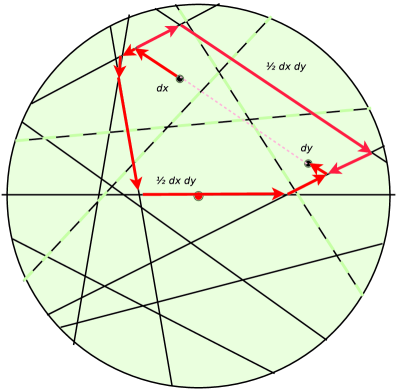
two possible routes given by the semiperimeter algorithm (see Figure 7).

3.1 First order calculations at the center

Recall (1) from the Introduction: the flow through the center is measured by the $4$-volume of $\mathcal{D}_{n}$, where

$$\mathcal{D}_{n}=\{(p^{-},p^{+})\in\operatorname{ball}(\mathbf{o},n)^{2}\dvtx p^{-}_{1}<p^{+}_{1},\mathbf{o}\in\partial\mathcal{C}(p^{-},p^{+})\},$$

and we seek to understand the large-$n$ statistical behavior of this $4$-volume. Indeed (bearing in mind that we have conditioned on there being a line through $\mathbf{o}$), the distribution of the total traffic through the origin $\mathbf{o}$ is given by the distribution of

$$T_{n} = \frac{1}{2}\int\!\!\int\mathbb{I}_{[(p^{-},p^{+})\in\mathcal{D}_{n}]}\,{d}p^{-}\,{d}p^{+}$$

$$= \frac{1}{2}\int\!\!\int_{\operatorname{ball}(\mathbf{o},n)^{2}}\mathbb{I}_{[p^{-}_{1}<p^{+}_{1},\mathbf{o}\in\partial\mathcal{C}(p^{-},p^{+})]}\,{d}p^{-}\,{d}p^{+}.$$

The mean can be obtained asymptotically using direct arguments.

Theorem 5

The mean flow through a line at the center is given by

$$\mathbb{E}[T_{n}]=\int_{0}^{\pi}\int_{0}^{n}\int_{0}^{n}\exp\biggl{(}-\frac{1}{2}(r+s-\rho)\biggr{)}r\,{d}r\,s\,{d}s\,\theta\,{d}\theta,$$ (24)

where $\rho=\sqrt{r^{2}+s^{2}+2rs\cos\theta}$. Asymptotically, as $n\to\infty$,

$$\mathbb{E}[T_{n}]\sim 2n^{3}.$$ (25)

Equation (24) follows from simple stochastic geometry of Poisson line processes (illustrated in Figure 8), taking care not to double-count flow between the unordered points $p^{+}$ and $p^{-}$. Note that when $p^{+}$ and $p^{-}$ are on opposing sides of the line conditioned to hit the origin, none of the flows between these two points will run through the origin. Indeed, mean flows between points $p^{+}$, $p^{-}$ in the upper half-plane will account for exactly half the total mean flow through the origin.

Figure 8: Illustration of the geometry represented by the multiple integral in (24) using $r$, $s$, $\theta$. The segment $p^{-}p^{+}$ is not separated from the origin $\mathbf{o}$ exactly when no lines of the line process pass through both of $\mathbf{o}p^{-}$ and $\mathbf{o}p^{+}$.

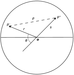
The asymptotics follow by application of scaling by $n$, the symmetry between $s$ and $r$, and the inequality $\sqrt{1-2z}\leq 1-z$ for $z\geq\frac{1}{2}$. Indeed,

$$\mathbb{E}[T_{n}] = 2n^{4}\int_{0}^{\pi}\int_{0}^{1}\int_{0}^{s}\exp\biggl{(}-\frac{n}{2}(r+s-\rho)\biggr{)}r\,{d}r\,s\,{d}s\,\theta\,{d}\theta$$

$$= 2n^{4}\int_{0}^{\pi}\int_{0}^{1}\int_{0}^{1}\exp\biggl{(}-\frac{ns}{2}\bigl{(}r+1-\sqrt{r^{2}+1+2r\cos\theta}\bigr{)}\biggr{)}r\,{d}r\,s^{3}\,{d}s\,\theta\,{d}\theta.$$

The region of the integral corresponding to $\int_{\theta_{n}}^{\pi/2}\int_{0}^{1}\int_{0}^{1}$ (for $\theta_{n}>0$) is bounded above by

$$2n^{4}\int_{\theta_{n}}^{\pi}\int_{0}^{1}\int_{0}^{1}\exp\biggl{(}-\frac{ns}{2}\bigl{(}r+1-\sqrt{r^{2}+1+2r\cos\theta}\bigr{)}\biggr{)}r\,{d}r\,s^{3}\,{d}s\theta\,{d}\theta$$

$$\qquad\leq 2n^{4}\int_{\theta_{n}}^{\pi}\int_{0}^{1}\int_{0}^{1}\exp\biggl{(}-\frac{nsr}{2(r+1)}(1-\cos\theta)\biggr{)}r\,{d}r\,s^{3}\,{d}s\,\theta\,{d}\theta$$

$$\qquad\leq(\pi-\theta_{n})^{2}n^{4}\int_{0}^{1}\int_{0}^{1}\exp\biggl{(}-\frac{nsr}{2(r+1)}(1-\cos\theta_{n})\biggr{)}r\,{d}r\,s^{3}\,{d}s$$

$$\qquad\leq(\pi-\theta_{n})^{2}n^{4}\int_{0}^{1}\int_{0}^{\infty}\exp\biggl{(}-\frac{nsr}{4}(1-\cos\theta_{n})\biggr{)}r\,{d}r\,s^{3}\,{d}s$$

$$\qquad=(\pi-\theta_{n})^{2}\biggl{(}\frac{4}{1-\cos\theta_{n}}\biggr{)}^{2}n^{2}\int_{0}^{1}s\,{d}s=8\biggl{(}\frac{\pi-\theta_{n}}{1-\cos\theta_{n}}\biggr{)}^{2}n^{2}.$$

Consider the region $\int_{0}^{\theta_{n}}\int_{0}^{1}\int_{0}^{1}$. Using a Taylor series expansion of $1-\sqrt{1-2z}$ and the approximation $\theta/\sin\theta\searrow 1$ as $\theta\searrow 0$ (so long as $0<\theta<\pi/2$), we deduce that

$$\mathbb{E}[T_{n}] \sim 2n^{4}\int_{0}^{1}\int_{0}^{1}\int_{0}^{\infty}\exp\biggl{(}-\frac{nsr}{2(1+r)}u\biggr{)}\,{d}u\,s^{3}\,{d}s\,r\,{d}r$$

$$= 2n^{4}\int_{0}^{1}\int_{0}^{1}\frac{2(1+r)}{nsr}s^{3}\,{d}s\,r\,{d}r=2n^{3}.$$

Taking some extra care over the analysis, it is possible to bound the order of the error in (25). We state this without proof.

Corollary 6

The asymptotic in Theorem 5 can be sharpened to

$$\mathbb{E}[T_{n}]\sim 2n^{3}+O\bigl{(}n^{2}\sqrt{n}\bigr{)}\qquad\mbox{as }n\to\infty.$$

3.2 Mean flow averaged over entire disc

Regional variation of expected flow over the disc is to be expected: flow at the boundaries should be lower than at the center. Indeed, one can calculate the mean flow per unit length in the network as follows.

The mean total length of the intersection of the Poisson line pattern with the disc is given by (mean number of lines hitting disk) $\times$ average intersection length:

$$(2\pi n)\times\biggl{(}\frac{1}{2n}\int_{-n}^{n}2\sqrt{n^{2}-x^{2}}\,{d}x\biggr{)}=\frac{\pi^{2}n^{2}}{2},$$

and this is therefore the mean total network length in the disc.

On the other hand, the mean Euclidean distance between two independent uniformly random points in the disc is given by

$$\frac{1}{\pi n^{2}}\int_{0}^{2\pi}\int_{0}^{n}\frac{1}{\pi n^{2}}\int_{0}^{2\pi}\int_{0}^{n}\sqrt{u^{2}+v^{2}-2uv\cos(\alpha-\beta)}v\,{d}v\,{d}\beta\,u\,{d}u\,{d}\alpha$$

$$\qquad=\frac{8n}{5\pi}\int_{0}^{\pi}\int_{0}^{1}\sqrt{u^{2}+1-2u\cos\theta}u\,{d}u\,{d}\theta$$

$$\qquad=\frac{8n}{5\pi}\int_{0}^{\pi/2}\int_{0}^{2\cos\phi}s^{2}\,{d}s\,{d}\phi=\frac{128}{45\pi}n,$$

where the first step uses various symmetries and rescaling, and the second step changes to polar coordinates based at $u=1$ and $\theta=0$ in an implicit use of Crofton’s method. [This calculation is a special case of a classic calculation in geometric probability, surveyed in Santaló (1976), Chapter 12.7 Note (6).] By the previous results on lengths of network geodesics, the mean network distance differs only by an extra logarithmic contribution.

Hence, the mean flow per unit length, if each pair of points exchanges just one infinitesimal unit of traffic and this is averaged over the network, is asymptotic to

$$\frac{1}{2}\frac{(\pi n^{2})^{2}\times({128}/({45\pi}))n}{{\pi^{2}n^{2}}/{2}}=\frac{128}{45\pi}n^{3}=1.9052\ldots n^{3}.$$

This analysis does not take account of routes which move outside the perimeter of the disc; however, the effect of these routes can be shown to be negligible. [The key observation is based on Theorem 1: if both source and destination nodes $p^{\pm}$ are at least $2\sqrt{(1+\varepsilon)n\log n}$ from the perimeter of a disc of radius $n$, and $n$ is large enough, then points outside the disc have probability at most $O(n^{-(1+\varepsilon)})$ of lying within $\mathcal{C}(p^{-},p^{+})$. Thus, mean total length outside the disc is a boundary rather than an area effect.] In conclusion, and unsurprisingly, mean flow over a typical line is slightly smaller than mean flow over a line at the center of the disc.

3.3 An improper anisotropic limiting line process

We can represent the scaling limit of the distribution of traffic flow through the center of the Poissonian city by using an improper stationary anisotropic Poisson line process.

We use the alternate coordinatization of a unit rate stationary isotropic Poisson line process, as in Figure 9, using coordinate $x$ for the intersection along the $x$-axis and $\theta$ for line direction. The $x$-axis intersections then form a stationary Poisson point process, while the angle density is $\frac{1}{2}\sin\theta$ for $0<\theta<\pi$.

Figure 9: The Poisson line process can be represented in terms of a Poisson process of points scattered along the $x$-axis, through each of which there runs a line making an angle $\theta\in(0,\pi)$ with the $x$-axis, with density $\frac{1}{2}\sin\theta$. Here, we show this against a backdrop of the disc $\operatorname{ball}(\mathbf{o},n)$.

Figure 10: This illustrates the result of scaling by $1/n$ in the $x$-direction and $1/\sqrt{n}$ in the $y$-direction.

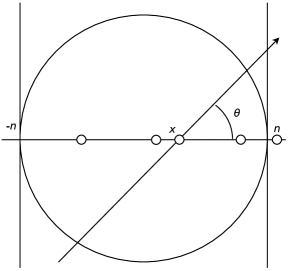
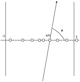
Rescale to shrink the $x$-axis by a factor of $1/n$, so $\widetilde{x}=x/n$. Guided by previous results, shrink the $y$-axis by a different amount, $1/\sqrt{n}$, so $\widetilde{y}=y/\sqrt{n}$. Thus, $\theta$ is transformed into a new angle $\phi$ (see Figure 10), where

$$\tan\phi=\sqrt{n}\tan\theta.$$

In the new coordinates of $\widetilde{x}$ and $\phi$, the line process can be parametrized as a nonstationary Poisson point process on $\widetilde{x}\dvtx\phi$ space with intensity

$$\frac{1}{2}\frac{\tan\phi\sec^{2}\phi}{(1+({1}/{n})\tan^{2}\phi)^{3/2}}\,{d}\widetilde{x}\,{d}\phi\nearrow\frac{1}{2}\tan\phi\sec^{2}\phi\,{d}\widetilde{x}\,{d}\phi.$$

We can represent this as a coupling construction: based on an improper stationary anisotropic Poisson line process with intensity $\frac{1}{2}\tan\phi\sec^{2}\phi\,{d}\widetilde{x}\,{d}\phi$ in $\widetilde{x}\dvtx\phi$ coordinates, we can achieve a proper stationary isotropic Poisson line process at scale $n$ by randomly thinning the lines with retention probability depending monotonically on the line slope.

Moreover, this limiting object may be cleanly represented using a further set of coordinates. Represent each line of the line process by its intercepts $y_{+}$ and $y_{-}$ on the vertical axes $x=1$ and $x=-1$ (see Figure 11). The intensity then becomes

$$\tfrac{1}{4}\,{d}y_{+}\,{d}y_{-}.$$

In particular, while the new improper Poisson line process is anisotropic, it nevertheless does possess special affine shear symmetries, namely the symmetries produced by those area-preserving linear transformations which leave all vertical axes invariant.

Figure 11: This illustrates the parametrization of lines from the improper limiting line process as intercepts on two parallel $y$-axes.

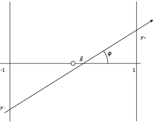
This construction enables us to identify the limiting behavior for $T_{n}$, as follows.

Theorem 7

The scaled quantity $T_{n}/n^{3}$ has a limiting distribution given by the analogous flow at the center for the limiting improper stationary anisotropic Poisson line process given above.

Indeed, we can relate scaled finite-$n$ instances to the limiting case by a coupling argument involving the addition of further lines; however, the resulting almost sure limit is not monotonically decreasing since it will involve a double integral [as in (3.1)] taken over ever-increasing regions of the vertical strip in Figure 11.

Before proving this theorem, we show that the mean flow at the center for this limit is in agreement with the asymptotics given in Theorem 5.

Lemma 8

The flow at the center for the limiting improper stationary anisotropic Poisson line process given above has mean value $2$.

Consider first the probability that the line segment from $(-a,t)$ to $(u,t)$ is not separated from the origin by the improper line process. The mean measure of lines implementing such a separation (measured using the intensity measure of the improper process) is $A+B+C$, where the contribution $A$ arises from separating lines hitting the upper-left shaded triangle in Figure 12, the contribution $C$ arises from those hitting the upper-right shaded triangle in Figure 12 and $B$ is derived from the contribution of the remaining separating lines.

Figure 12: Computing the mean flow through the center for the flow based on the improper anisotropic line process limit.

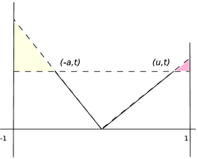
Then,

$$A=\frac{1}{4}\int_{t}^{t/a}\biggl{(}\biggl{(}s-2\frac{s-t}{1-a}\biggr{)}+s\biggr{)}\,{d}s=\frac{t^{2}}{4}\biggl{(}\frac{1}{a}-1\biggr{)}$$

and, similarly, $C=\frac{t^{2}}{4}(\frac{1}{u}-1)$. Finally,

$$B=\frac{1}{4}\int_{-t}^{t}(t+s)\,{d}s=2\frac{t^{2}}{4}.$$

Consequently,

$$A+B+C=\frac{t^{2}}{4}\biggl{(}\frac{1}{a}+\frac{1}{u}\biggr{)}.$$

Since we are dealing with a Poisson process, the required probability of the line segment from $(-a,t)$ to $(u,t)$ not being separated from the origin is

$$\exp\biggl{(}-\frac{t^{2}}{4}\biggl{(}\frac{1}{a}+\frac{1}{u}\biggr{)}\biggr{)}.$$ (26)

Consider the special affine shear symmetries which leave the $x=0$ axis fixed. Because of this symmetry group, it follows that the probability of the line segment from $(-a,b)$ to $(u,v)$ not being separated from the origin agrees with (26) when the line segment from $(-a,b)$ to $(u,v)$ passes through $(0,t)$. This occurs when $t=\frac{bu+av}{a+u}$; moreover, if we set $s=b-v$, then ${d}t\,{d}s={d}b\,{d}v$. Accordingly, the mean $4$-volume of the region representing the flow through the center is given by

$$\int_{0}^{1}\int_{0}^{1}\int_{0}^{\infty}\int_{-(({a+u})/{a})t}^{(({a+u})/{u})t}\exp\biggl{(}-\frac{t^{2}}{4}\biggl{(}\frac{1}{a}+\frac{1}{u}\biggr{)}\biggr{)}\,{d}s\,{d}t\,{d}a\,{d}u$$

$$\qquad=\int_{0}^{1}\int_{0}^{1}\int_{0}^{\infty}(a+u)\biggl{(}\frac{1}{a}+\frac{1}{u}\biggr{)}\exp\biggl{(}-\frac{t^{2}}{4}\biggl{(}\frac{1}{a}+\frac{1}{u}\biggr{)}\biggr{)}t\,{d}t\,{d}a\,{d}u$$

$$\qquad=2\int_{0}^{1}\int_{0}^{1}(a+u)\,{d}a\,{d}u=2.$$

Proof of Theorem 7 Consider the affine shear transformation $\mathcal{T}_{n}\dvtx[-1$, $1]\times(0,\infty)\to[-1,1]\times(0,\infty)$ given by $\mathcal{T}_{n}(u,v)=(nu,\sqrt{n}v)$. Define coupled random functions

$$\displaystyle I_{n}\dvtx\bigl{(}[-1,0]\times(0,\infty)\bigr{)}\times\bigl{(}[0,1]\times(0,\infty)\bigr{)}\to\{0,1\},$$

$$\displaystyle I_{n}(p,q)=\mathbb{I}_{[\mathcal{T}_{n}p\in\operatorname{ball}(\mathbf{o},n)]}\mathbb{I}_{[\mathcal{T}_{n}q\in\operatorname{ball}(\mathbf{o},n)]}\mathbb{I}_{[\mathbf{o}\in\mathcal{C}(\mathcal{T}_{n}p,\mathcal{T}_{n}q)]}.$$

So, $I_{n}$ depends implicitly on the underlying Poisson line process: the previously described coupling construction shows that we can couple different Poisson line processes for each $n$ so as to arrange that $I_{n}(p,q)\to I(p,q)$ almost surely for Lebesgue almost all $p$, $q$, where $I(p,q)$ is given by an analogous construction based on the limiting improper anisotropic Poisson line process, and not using $\mathcal{T}_{n}$. Moreover, we can realize $T_{n}$ using

$$T_{n}/n^{3}=\frac{1}{2}\int\!\!\int I_{n}(p,q)\,{d}p\,{d}q.$$

From Theorem 5 and Lemma 8, it follows that

$$\mathbb{E}\biggl{[}\frac{1}{2}\int\!\!\int I_{n}(p,q)\,{d}p\,{d}q\biggr{]}\to\mathbb{E}\biggl{[}\frac{1}{2}\int\!\!\int I(p,q)\,{d}p\,{d}q\biggr{]}=2.$$

On the other hand, if we restrict consideration to the finite measure space $\Omega\times([-1,0]\times(0,K))\times([0,1]\times(0,K))$ for any fixed $K$, then we may deduce $L^{1}$-convergence of $I_{n}$ to $I$ via the dominated convergence theorem since the indicator functions $I_{n}$ are bounded. [Here, $(\Omega,\mathfrak{F},\mathbb{P})$ is the underlying probability space.]

It then follows from nonnegativity of the $I_{n}$, $I$ that we can apply Fatou’s lemma to deliver $L^{1}$-convergence on all of $\Omega\times([-1,0]\times(0,\infty))\times([0,1]\times(0,\infty))$ and so can deduce convergence in distribution as required:

$$T_{n}/n^{3}=\frac{1}{2}{\int\!\!\int I_{n}(p,q)\,{d}p\,{d}q}\mathop{\to}_{\mathcal{D}}\frac{1}{2}{\int\!\!\int I(p,q)\,{d}p\,{d}q,}$$

viewed as random variables (functions of $\omega\in\Omega$).

Note that this proof also establishes uniform integrability of the sequence of random variables $\{T_{n}/n^{3}\dvtx n\geq 1\}$.

It is apparent from this construction that the limiting distribution is largely insensitive to modest variations in the geometry of the city [$\operatorname{ball}(\mathbf{o},n)$, or square of side $2n$, or$\ldots$]; however, we will not explore this here.

In principle it is possible that the limiting distribution of $T_{n}/n^{3}$ might be degenerate. That this is not the case follows rapidly from representation of the limit in terms of the improper anisotropic Poisson line process.

Corollary 9

The limiting distribution of $T_{n}/n^{3}$ is nondegenerate.

Let $E_{k}$ be the event

$$E_{k}=\biggl{[}\mbox{there is a line connecting }\{-1\}\times\biggl{[}0,\frac{1}{k}\biggr{]}\mbox{ to }\{+1\}\times\biggl{[}0,\frac{1}{k}\biggr{]}\biggr{]}.$$

Then, $E_{k}$ has positive probability for the improper anisotropic Poisson line process; moreover, $E_{1}$, $E_{2},\ldots$ form a monotonically decreasing sequence of events whose intersection is a null set. It follows from elementary measure theory that

$$\mathbb{E}\biggl{[}\frac{1}{2}\int\!\!\int I(p,q)\,{d}p\,{d}q;E_{k}\biggr{]}\to 0.$$

However, simple constructions show positivity of the conditional expectation

$$\mathbb{E}\biggl{[}\int\!\!\int I(p,q)\,{d}p\,{d}q\Big{|}E_{k}\biggr{]}>0$$

for each $k$. Because each event $E_{k}$ is of positive probability, it follows that for each $\varepsilon>0$, we can find $k$ such that

$$0<\mathbb{E}\biggl{[}\frac{1}{2}\int\!\!\int I(p,q)\,{d}p\,{d}q;E_{k}\biggr{]}<\varepsilon.$$

It follows that the random variable

$$\frac{1}{2}\int\!\!\int I(p,q)\,{d}p\,{d}q$$

cannot be deterministic, and this establishes nondegeneracy of the limiting distribution of $T_{n}/n^{3}$.

3.4 Higher order moments

We have established that one can produce a coupling construction to show that $T_{n}/n$ converges almost surely, and indeed in mean value, to the corresponding quantity for the improper stationary anisotropic line process. In fact, it is possible to establish convergence of moments of order $2-\epsilon$ for $\epsilon\in(0,2)$; computations show that the second moment $\mathbb{E}[T_{n}^{2}]$ is bounded by $\mathrm{const.}\times n^{6}$, hence a uniform integrability argument may be applied. The tiresomely complicated computations are omitted; we simply indicate the general approach. The second moment can be expressed using an eight-fold integral:

$$\int_{0}^{n}\int_{0}^{n}\int_{0}^{\pi}\int_{0}^{\theta}\int_{0}^{n}\int_{0}^{n}\int_{0}^{\pi}\int_{0}^{\phi}\mathbb{P}[E(r,s,\theta,\alpha,$$

$$\hskip 158.3ptu,v,\phi,\beta)]\,{d}\beta\,{d}\phi\,u\,{d}u\,v\,{d}v\,{d}\alpha\,{d}\theta\,r\,{d}r\,s\,{d}s,$$

where $E(r,s,\theta,\alpha,u,v,\phi,\beta)$ is the event that neither of two line segments [$(r,\alpha)$-$(s,\alpha+\pi-\theta)$ and $(u,\beta,)$-$(v,\beta+\pi-\phi)$ when written in polar coordinates] is separated from the origin by the line process (see Figure 13).

Figure 13: Illustration of the event $E(r,s,\theta,\alpha,u,v,\phi,\beta)$, which happens if neither of the segments $u\to v$, $r\to s$ is separated from the origin by the line process.

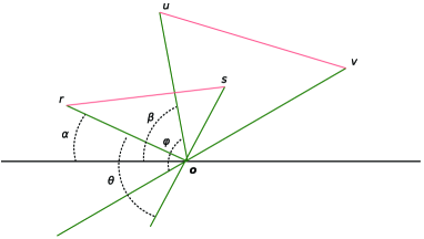
Analysis of this eight-fold integral is complicated because the probability

$$\mathbb{P}[E(r,s,\theta,\alpha,u,v,\phi,\beta)]$$

takes on around eight different analytical forms, according to the relative geometry of the line segments. Case-by-case mathematical analysis shows that the multiple integral is bounded by $\mathrm{const.}\times n^{6}$.

4 Comparison with a Manhattan city

It is natural to ask how the Poissonian city might compare with an alternate Manhattan city based on a more conventional Cartesian grid structure of roads (a “grid city”). Consider the case of a disc of radius $n$ furnished with roads arranged in a fixed unit-length grid structure. Suppose we wish to connect from the point at $-(u,v)$ to the point at $(x,y)$ (using Cartesian coordinates). If $u$, $v$, $x$ and $y$ are all nonnegative, then there is a wide variety of possible network geodesic connections. Working with the most direct analogy to the results described in Section 3, suppose that traffic from $-(u,v)$ to $(x,y)$ divides equally between the two extreme network geodesics running from $-(u,v)$ to $(x,y)$. Working to $O(n^{3})$ (allowing us to ignore some double-counting), the total traffic through $\mathbf{o}$ is made up of four contributions, arising from (i) $u=0,v>0$, (ii) $u>0,v=0$, (iii) $x=0,y>0$, (iv) $x>0,y=0$. Each case individually contributes a term of the form

$$2\mathop{\mathop{\sum\sum}_{(x,y)>0}}_{x^{2}+y^{2}\leq n^{2}}\frac{1}{2}n=\frac{\pi}{4}n^{3}+O(n^{2}),$$

where we omit the negligible contributions arising when there is just one network geodesic between source and destination. We can sum these contributions since the effect of double-counting is again negligible. Thus, the total flow through $\mathbf{o}$ is $\pi n^{3}+O(n^{2})$. If we fix our attention on total flow through one of the bonds attached to $\mathbf{o}$ (so as to establish comparability with the results of Section 3.1 for the Poissonian city), then we obtain $\frac{\pi}{2}n^{3}+O(n^{2})$, compared with mean flow for the Poissonian city of $2n^{3}$.

However, account needs to be taken of the greater total length of the grid network. Mean total network length produced by the unit intensity Poisson line process is $\frac{\pi^{2}n^{2}}{2}$, compared with $2\times\pi n^{2}$ for the unit grid structure. Thus, a comparable grid structure has to be based on segments of length $\frac{4}{\pi}$ rather than $1$. The flow produced through a bond attached to $\mathbf{o}$ by such a grid using the above protocol will be of order

$$\frac{(\pi n^{2})^{2}}{(\pi(({\pi}/{4})n)^{2})^{2}}\times\frac{\pi}{2}\biggl{(}\frac{\pi}{4}n\biggr{)}^{3}=2n^{3},$$

where the second term computes the flow through a center bond when rescaling from $n$ to $\frac{\pi}{4}n$, and the first factor is a correction to ensure that total traffic is $(\pi n^{2})^{2}$, not $(\pi(\frac{\pi}{4}n)^{2})^{2}$. Thus, the Poissonian city is comparable to this grid structure in terms of mean flow at the center. However, the grid structure with this protocol can be shown to have the undesirable feature that, asymptotically, a definite proportion of the total traffic (around 2%) occurs outside the disc.

In fact, we can also carry out calculations for a somewhat more demanding situation in which, asymptotically, the traffic stays within the disc, as in the case of the Poissonian city; instead of supposing the traffic to be divided equally between the two extreme network geodesics, we suppose that it is divided equally among all possible network geodesic connections. In effect, the actual network geodesic is chosen uniformly at random, and in that case the probability that the resulting network geodesic passes through the origin $(0,0)$ is

$$\frac{\mathbb{P}[\operatorname{Bin}(u+v,p)=u]\mathbb{P}[\operatorname{Bin}(x+y,p)=x]}{\mathbb{P}[\operatorname{Bin}(u+v+x+y,p)=u+x]}=\frac{{u+v\choose u}{x+y\choose x}}{{u+v+x+y\choose u+x}}.$$ (27)

Here, $p=\frac{1}{2}$, but the same result is in fact obtained for any $0<p<1$. Choosing $p=\frac{u+x}{u+v+x+y}$, so as to control the denominator, and applying Stirling’s formula, we can use a Taylor expansion to approximate this by

$$\frac{1}{\sqrt{2\pi}}\frac{(u+v+x+y)^{3/2}}{\sqrt{(u+v)(x+y)(u+x)(v+y)}}$$

(28)

$$\qquad\times{}\exp\biggl{(}-\frac{(u+v+x+y)(uy-xv)^{2}}{2(u+v)(x+y)(u+x)(v+y)}\biggr{)}.$$

Using polar coordinates based on an axis at $45^{\circ}$ to the Cartesian axes and a Gaussian approximation based on $\sin^{2}(\theta-\phi)\approx(\theta-\phi)^{2}$, we obtain a heuristic approximation for large $n$ for the flow between two opposing quadrants of the disc:

$$\mathop{\mathop{\sum\sum}_{u,v\geq 0}}_{u^{2}+v^{2}\leq n^{2}}\mathop{\mathop{\sum\sum}_{x,y\geq 0}}_{x^{2}+y^{2}\leq n^{2}}\frac{{u+v\choose u}{x+y\choose x}}{{u+v+x+y\choose u+x}}\approx 2n^{3}.$$ (29)

Conversion of this approach into a rigorous asymptotic argument would require close attention to detailed asymptotics of the Binomial distribution [Littlewood (1969), McKay (1989)]. However, there is an alternate argument which is more easily made rigorous: the expression (29) can be reexpressed in terms of a symmetric random walk $X$ as

$$\mathop{\mathop{\sum\sum}_{u,v\geq 0}}_{u^{2}+v^{2}\leq n^{2}}\mathop{\mathop{\sum\sum}_{x,y\geq 0}}_{x^{2}+y^{2}\leq n^{2}}\mathbb{P}[X_{u+v}=v-u|X_{u+v+x+y}=v-u+y-x].$$

Under the $\mathbb{Z}$-action $u\to u-1,v\to v+1,x\to x+1,y\to y+1$, a statistical pivot argument applied to the summand generates a probability distribution on even integers or odd integers according to the parity of $u+v$, $x+y$. An argument using the Hoeffding inequality quantifies how this probability distribution concentrates around its mode; the denominator is controlled by choosing the probability $\mathbb{P}[X_{n+1}=X_{n}-1]=p=\frac{u+x}{u+v+x+y}$. It can thus be shown that the asymptotic behavior of the quadruple sum is given by the number of $\mathbb{Z}$-orbits containing modal representatives close to the line between $-(u,v)$ and $(x,y)$. This number can be expressed as a sum susceptible to elementary asymptotic analysis, finally yielding a rigorous argument for the asymptotic given in (29).

Consider now the total flow through a unit-length bond $\ell$ connected to the origin. This will equal half the total flow through the origin, which itself can be viewed asymptotically as the sum of two equal components from two different pairs of opposing quadrants. Thus, this total flow is again asymptotic to $2n^{3}$.

Again, a grid structure comparable to the Poissonian city must be based on segments of length $\frac{4}{\pi}$ rather than $1$, and a scaling argument then shows that such a grid structure produces mean flow at the center which is asymptotic to $\frac{4}{\pi}\times 2n^{3}=2.54648\ldots n^{3}$. Thus, traffic through the center under this protocol is about $25\%$ higher in a comparable Manhattan city.

Geodesics in the Manhattan city are on average longer than those in the Poisson line process; we can in fact argue in a manner analogous to that of Section 3.2 to show that mean network distance between two independent uniformly random points in the disc will be asymptotic to

$$\frac{128}{45\pi}n\times\frac{1}{2\pi}\int_{0}^{2\pi}(|{\sin\theta}|+|{\cos\theta}|)\,{d}\theta=\frac{128}{45\pi}n\times\frac{4}{\pi},$$

so the mean network flow over the whole disc for the grid will again be about 25% greater than mean network flow for the Poisson line process.

Of course, the second order behaviors of the flows are rather different: flow at the center of the Poissonian city inherits asymptotically nondegenerate randomness from the random configuration of the Poisson line process, while a central limit argument shows that the flows at the centers of the two kinds of flow in Manhattan cities are asymptotically deterministic.

5 Complements and conclusion

In conclusion, we present some notes concerning complements and issues for further research, illustrating the potentially rich theory concerning the Poissonian city.

Empirical comparisons

Clearly, the Poissonian city does not accurately represent real cities; there will be variation both of geometry and of traffic flow. It would be interesting to make empirical comparisons with actual street map and traffic flow data, both in terms of network distance statistics compared with the results of Section 1.2 and (much more demanding from a data collection point of view) in terms of flow statistics compared with the results of Section 3. One would expect qualitative agreement at best, rather than quantitative, in view of the strong stochastic assumptions implicit in the Poissonian city. Note, however, that the results on the asymptotic statistics of flow at the center (Theorem 7) reflect variation across a sample of different cities, rather than within a particular city.

Lower bounds on path length

Compare the lower bound of Section 2.3, Theorem 4, with the more general lower bound of Aldous and Kendall [(2008), Theorem 2], which holds for all connecting networks using total network length proportional to $n$ based on patterns of nodes in a square $[0,\sqrt{n}]^{2}$ satisfying a certain quantitative equidistribution condition (related to an intuitive coupling construction). The Aldous and Kendall (2008) result provides an $\Omega(\sqrt{\log n})$ bound on excess, whereas Theorem 4 uses detailed properties of Poisson line process networks to establish a $\mathrm{const.}\times\log n$ lower bound. A natural question is whether there are any network constructions which provide sub-logarithmic mean excess for appropriately equidistributed patterns of nodes, or whether, on the other hand, the general lower bound can be improved.

Analytical characterization of limit

The stochastic geometric construction of the limit distribution for flow in the center of a Poissonian city using an improper stationary anisotropic Poisson line process (Section 3.3) is explicit and lends itself to simulation; however, it would be helpful also to have an analytic expression, or at least characterization, of the limiting distribution. This seems difficult. Note that we can produce a stochastic representation of the moment generating function $M(p)$ of the limit distribution in terms of the following probability: consider a Poisson process of intensity $\alpha$ of pairs of points on $[-1,1]\times(0,\infty)$. Then, $M(-\alpha)$ is the probability that no pairs produced by this process are separated from the origin by lines of the improper stationary anisotropic Poisson line process. Similar representations are of use in perfect simulation of area-interaction point process models [Kendall (1997)] and exact simulation of diffusions [Beskos and Roberts (2005)]. However, in the current case it is not yet clear whether this offers any progress toward simulation methods or delivering a useful analytical representation.

A slightly easier question is whether the convergence of $T_{n}/n^{3}$ to the limit distribution holds for all moments. Again, at present no progress on this can be offered beyond the work noted in Section 3.4.

Aggregation issues

What can we say about similar situations where the distribution of nodes generating the flow is nonuniform? Or even when the nodes generating the flows lie along the Poisson line process itself (thus precluding the need for the “cross country” plumbing otherwise required to get onto the network)? Considerations of this kind are latent in the early work of Davidson (1974), and it would be interesting to see them applied in the more quantitative setting of the present work. It is possible that the coupling construction in Aldous and Kendall (2008) would be of use here.

Three dimensions and higher

In higher dimensions, one needs to consider what kind of network is being deployed. One might, for example, consider the edge process of a Poisson hyperplane tessellation or, alternatively, one might consider network geodesics constrained to lie on the union of all faces of the tessellation. In the second case, one can derive upper bounds on excess by considering the derivative planar problem obtained by taking a $2$-plane slice through the source and destination nodes; it is then a question of how much the excess may be reduced by varying the orientation of the slice, and it is a further question as to whether the excess can be further substantially reduced by using paths which do not lie wholly on the slicing plane. It may be possible to make progress in the first case by adopting the growth process approach of Section 2.2.

Note that Böröczky and Schneider (2010) describe higher-dimensional results for similar problems; however, their results concern standard stereological quantities, while we would need results involving infima of lengths of regular curves on the boundaries of Poisson cells.

Moving beyond line processes

Certainly, one can conceive of results for situations based on processes which approximate Poisson line processes; Boolean models based on long line segments or fiber processes for which there is strong control of total fiber curvature. It would be particularly interesting to determine the extent to which Poissonian cities and Manhattan cities represent two extremes of a suitable class of models.

User equilibrium

The notion of UE [user equilibrium, Wardrop (1952), contemporary with the related notion of Nash equilibrium] supposes that each user has a utility structure for choosing which route they might take based on travel time, which is affected not only by available route lengths but also by flow along the routes. Interest is then focused on systems of choices by users which result in user equilibrium; no one user can obtain a shorter route by varying their own route. Explorations have already been made in the context of queueing theory; see, for example, Calvert, Solomon and Ziedins (1997), who consider the effect of augmenting a simple queueing network and Afimeimounga, Solomon and Ziedins (2005), who consider a system of interactions between a $\cdot/M/1$ queue and a $\cdot/N^{(N)}/\infty$ batch queue. There are interesting possibilities in the context of the Poissonian city, for example, considering that traffic from $p^{-}$ to $p^{+}$ chooses each of the two possible routes prescribed by the semiperimeter algorithm according to considerations both of length and of integrated total flow along the routes.

Such problems are naturally formulated in terms of phase transitions in statistical mechanics, perhaps using the improper stationary anisotropic Poisson line process of Section 3.3.

References

- Afimeimounga, Solomon and Ziedins (2005) {barticle}[author] \bauthor\bsnmAfimeimounga, \bfnmHeti\binitsH., \bauthor\bsnmSolomon, \bfnmWiremu\binitsW. and \bauthor\bsnmZiedins, \bfnmIlze\binitsI. (\byear2005). \btitleThe Downs–Thomson paradox: Existence, uniqueness and stability of user equilibria. \bjournalQueueing Syst. \bvolume49 \bpages321–334. \bmrnumberMR2149647 (2006g:60134) \endbibitem
- Aldous and Kendall (2008) {barticle}[author] \bauthor\bsnmAldous, \bfnmDavid J.\binitsD. J. and \bauthor\bsnmKendall, \bfnmWilfrid S.\binitsW. S. (\byear2008). \btitleShort-length routes in low-cost networks via Poisson line patterns. \bjournalAdv. in Appl. Probab. \bvolume40 \bpages1–21. \bmrnumberMR2411811 (2009f:60018) \endbibitem
- Alsmeyer, Iksanov and Rœsler (2009) {barticle}[author] \bauthor\bsnmAlsmeyer, \bfnmGerold\binitsG., \bauthor\bsnmIksanov, \bfnmAlex\binitsA. and \bauthor\bsnmRœsler, \bfnmUwe\binitsU. (\byear2009). \btitleOn distributional properties of perpetuities. \bjournalJ. Theoret. Probab. \bvolume22 \bpages666–682. \bmrnumberMR2530108 \endbibitem
- Ambartzumian (1990) {bbook}[author] \bauthor\bsnmAmbartzumian, \bfnmR. V.\binitsR. V. (\byear1990). \btitleFactorization Calculus and Geometric Probability. \bpublisherCambridge Univ. Press, \baddressCambridge. \bmrnumberMR1075011 (92b:60013) \endbibitem
- Baccelli, Tchoumatchenko and Zuyev (2000) {barticle}[author] \bauthor\bsnmBaccelli, \bfnmF.\binitsF., \bauthor\bsnmTchoumatchenko, \bfnmK.\binitsK. and \bauthor\bsnmZuyev, \bfnmS.\binitsS. (\byear2000). \btitleMarkov paths on the Poisson–Delaunay graph with applications to routing in mobile networks. \bjournalAdv. in Appl. Probab. \bvolume32 \bpages1–18. \bmrnumberMR1765174 (2001k:60010) \endbibitem
- Baricz (2008) {barticle}[author] \bauthor\bsnmBaricz, \bfnmÁrpád\binitsÁ. (\byear2008). \btitleMills’ ratio: Monotonicity patterns and functional inequalities. \bjournalJ. Math. Anal. Appl. \bvolume340 \bpages1362–1370. \bmrnumberMR2390935 \endbibitem
- Bertoin and Yor (2001) {barticle}[author] \bauthor\bsnmBertoin, \bfnmJean\binitsJ. and \bauthor\bsnmYor, \bfnmMarc\binitsM. (\byear2001). \btitleOn subordinators, self-similar Markov processes and some factorizations of the exponential variable. \bjournalElectron. Comm. Probab. \bvolume6 \bpages95–106 (electronic). \bmrnumberMR1871698 (2002k:60097) \endbibitem
- Bertoin and Yor (2002) {barticle}[author] \bauthor\bsnmBertoin, \bfnmJean\binitsJ. and \bauthor\bsnmYor, \bfnmMarc\binitsM. (\byear2002). \btitleOn the entire moments of self-similar Markov processes and exponential functionals of Lévy processes. \bjournalAnn. Fac. Sci. Toulouse Math. (6) \bvolume11 \bpages33–45. \bmrnumberMR1986381 (2004d:60119) \endbibitem
- Bertoin and Yor (2005) {barticle}[author] \bauthor\bsnmBertoin, \bfnmJean\binitsJ. and \bauthor\bsnmYor, \bfnmMarc\binitsM. (\byear2005). \btitleExponential functionals of Lévy processes. \bjournalProbab. Surv. \bvolume2 \bpages191–212 (electronic). \bmrnumberMR2178044 (2007b:60116) \endbibitem
- Beskos and Roberts (2005) {barticle}[author] \bauthor\bsnmBeskos, \bfnmA.\binitsA. and \bauthor\bsnmRoberts, \bfnmG. O.\binitsG. O. (\byear2005). \btitleExact simulation of diffusions. \bjournalAnn. Appl. Probab. \bvolume15 \bpages2422–2444. \bmrnumberMR2187299 (2006e:60111) \endbibitem
- Birnbaum (1942) {barticle}[author] \bauthor\bsnmBirnbaum, \bfnmZ. W.\binitsZ. W. (\byear1942). \btitleAn inequality for Mill’s ratio. \bjournalAnn. Math. Statist. \bvolume13 \bpages245–246. \bmrnumberMR0006640 (4,19b) \endbibitem
- Böröczky and Schneider (2010) {barticle}[author] \bauthor\bsnmBöröczky, \bfnmKároly J.\binitsK. J. and \bauthor\bsnmSchneider, \bfnmRolf\binitsR. (\byear2010). \btitleThe mean width of circumscribed random polytopes. \bjournalCanad. Math. Bull. \bvolume53 \bpages614–628. \endbibitem
- Cabo and Groeneboom (1994) {barticle}[author] \bauthor\bsnmCabo, \bfnmA. J.\binitsA. J. and \bauthor\bsnmGroeneboom, \bfnmP.\binitsP. (\byear1994). \btitleLimit theorems for functionals of convex hulls. \bjournalProbab. Theory Related Fields \bvolume100 \bpages31–55. \bmrnumberMR1292189 (95g:60017) \endbibitem
- Calvert, Solomon and Ziedins (1997) {barticle}[author] \bauthor\bsnmCalvert, \bfnmBruce\binitsB., \bauthor\bsnmSolomon, \bfnmWiremu\binitsW. and \bauthor\bsnmZiedins, \bfnmIlze\binitsI. (\byear1997). \btitleBraess’s paradox in a queueing network with state-dependent routing. \bjournalJ. Appl. Probab. \bvolume34 \bpages134–154. \bmrnumberMR1429062 (98f:60182) \endbibitem
- Davidson (1974) {bincollection}[author] \bauthor\bsnmDavidson, \bfnmRollo\binitsR. (\byear1974). \btitleLine-processes, roads, and fibres. In \bbooktitleStochastic Geometry (A Tribute to the Memory of Rollo Davidson) (\beditorE. F. Harding and D. G. Kendall, eds.) \bpages248–251. \bpublisherWiley, \baddressLondon. \bmrnumberMR0358975 (50 ##11431) \endbibitem
- Dufresne (1990) {barticle}[author] \bauthor\bsnmDufresne, \bfnmDaniel\binitsD. (\byear1990). \btitleThe distribution of a perpetuity, with applications to risk theory and pension funding. \bjournalScand. Actuar. J. \bvolume1-2 \bpages39–79. \bmrnumberMR1129194 (92i:62195) \endbibitem
- Goldie and Grübel (1996) {barticle}[author] \bauthor\bsnmGoldie, \bfnmCharles M.\binitsC. M. and \bauthor\bsnmGrübel, \bfnmRudolf\binitsR. (\byear1996). \btitlePerpetuities with thin tails. \bjournalAdv. in Appl. Probab. \bvolume28 \bpages463–480. \bmrnumberMR1387886 (97f:60124) \endbibitem
- Groeneboom (1988) {barticle}[author] \bauthor\bsnmGroeneboom, \bfnmPiet\binitsP. (\byear1988). \btitleLimit theorems for convex hulls. \bjournalProbab. Theory Related Fields \bvolume79 \bpages327–368. \bmrnumberMR959514 (89j:60024) \endbibitem
- Hitczenko and Wesołowski (2009) {barticle}[author] \bauthor\bsnmHitczenko, \bfnmPaweł\binitsP. and \bauthor\bsnmWesołowski, \bfnmJacek\binitsJ. (\byear2009). \btitlePerpetuities with thin tails revisited. \bjournalAnn. Appl. Probab. \bvolume19 \bpages2080–2101. \bmrnumberMR2588240 \endbibitem
- Kellerer (1992) {bmisc}[author] \bauthor\bsnmKellerer, \bfnmH. G.\binitsH. G. (\byear1992). \btitleErgodic behaviour of affine recursions III: Positive recurrence and null recurrence. \bnoteTechnical report, Math. Inst. Univ. München, Theresienstrasse 39, 8000 München, Germany. \endbibitem
- Kendall (1997) {bincollection}[vtex] \bauthor\bsnmKendall, \bfnmWilfrid S.\binitsW. S. (\byear1997). \btitleOn some weighted Boolean models. In \bbooktitleAdvances in Theory and Applications of Random Sets (\beditorD. Jeulin, ed.) \bpages105–120. \bpublisherWorld Scientific, \baddressSingapore. \bmrnumberMR1654418 \endbibitem
- Kendall (2008) {barticle}[author] \bauthor\bsnmKendall, \bfnmWilfrid S.\binitsW. S. (\byear2008). \btitleNetworks and Poisson line patterns: Fluctuation asymptotics. \bjournalOberwolfach Rep. \bvolume5 \bpages2670–2672. \endbibitem
- Lamperti (1972) {barticle}[author] \bauthor\bsnmLamperti, \bfnmJohn\binitsJ. (\byear1972). \btitleSemi-stable Markov processes. I. \bjournalZ. Wahrsch. Verw. Gebiete \bvolume22 \bpages205–225. \bmrnumberMR0307358 (46 ##6478) \endbibitem
- Littlewood (1969) {barticle}[author] \bauthor\bsnmLittlewood, \bfnmJ. E.\binitsJ. E. (\byear1969). \btitleOn the probability in the tail of a binomial distribution. \bjournalAdv. in Appl. Probab. \bvolume1 \bpages43–72. \bmrnumberMR0240858 (39 ##2203) \endbibitem
- McKay (1989) {barticle}[author] \bauthor\bsnmMcKay, \bfnmBrendan D.\binitsB. D. (\byear1989). \btitleOn Littlewood’s estimate for the binomial distribution. \bjournalAdv. in Appl. Probab. \bvolume21 \bpages475–478. \bmrnumberMR997736 (90k:60030) \endbibitem
- Miles (1964) {barticle}[author] \bauthor\bsnmMiles, \bfnmR. E.\binitsR. E. (\byear1964). \btitleRandom polygons determined by random lines in a plane. \bjournalProc. Natl. Acad. Sci. USA \bvolume52 \bpages901–907. \bmrnumberMR0168000 (29 ##5265) \endbibitem
- Narasimhan and Smid (2007) {bbook}[author] \bauthor\bsnmNarasimhan, \bfnmGiri\binitsG. and \bauthor\bsnmSmid, \bfnmMichiel\binitsM. (\byear2007). \btitleGeometric Spanner Networks. \bpublisherCambridge Univ. Press, \baddressCambridge. \bmrnumberMR2289615 (2009b:68002) \endbibitem
- Prömel and Steger (2002) {bbook}[author] \bauthor\bsnmPrömel, \bfnmHans Jürgen\binitsH. J. and \bauthor\bsnmSteger, \bfnmAngelika\binitsA. (\byear2002). \btitleThe Steiner Tree Problem: A Tour Through Graphs, Algorithms, and Complexity. \bpublisherFriedr. Vieweg & Sohn, \baddressBraunschweig. \bmrnumberMR1891564 (2003a:05047) \endbibitem
- Rebolledo (1980) {barticle}[author] \bauthor\bsnmRebolledo, \bfnmRolando\binitsR. (\byear1980). \btitleCentral limit theorems for local martingales. \bjournalZ. Wahrsch. Verw. Gebiete \bvolume51 \bpages269–286. \bmrnumberMR566321 (81g:60023) \endbibitem
- Rényi and Sulanke (1968) {barticle}[author] \bauthor\bsnmRényi, \bfnmA.\binitsA. and \bauthor\bsnmSulanke, \bfnmR.\binitsR. (\byear1968). \btitleZufällige konvexe Polygone in einem Ringgebiet. \bjournalZ. Wahrsch. Verw. Gebiete \bvolume9 \bpages146–157. \bmrnumberMR0229272 (37 ##4846) \endbibitem
- Sampford (1953) {barticle}[author] \bauthor\bsnmSampford, \bfnmM. R.\binitsM. R. (\byear1953). \btitleSome inequalities on Mill’s ratio and related functions. \bjournalAnn. Math. Statist. \bvolume24 \bpages130–132. \bmrnumberMR0054890 (14,995g) \endbibitem
- Santaló (1976) {bbook}[author] \bauthor\bsnmSantaló, \bfnmLuis A.\binitsL. A. (\byear1976). \btitleIntegral Geometry and Geometric Probability. \bpublisherAddison-Wesley, \baddressReading, MA. \bnoteWith a foreword by Mark Kac, Encyclopedia of Mathematics and its Applications, Vol. 1. \bmrnumberMR0433364 (55 ##6340) \endbibitem
- Steele (1997) {bbook}[author] \bauthor\bsnmSteele, \bfnmJ. Michael\binitsJ. M. (\byear1997). \btitleProbability theory and combinatorial optimization. \bseriesCBMS-NSF Regional Conference Series in Applied Mathematics \bvolume69. \bpublisherSIAM, \baddressPhiladelphia, PA. \bmrnumberMR1422018 (99d:60002) \endbibitem
- Stoyan, Kendall and Mecke (1995) {bbook}[author] \bauthor\bsnmStoyan, \bfnmD.\binitsD., \bauthor\bsnmKendall, \bfnmWilfrid S.\binitsW. S. and \bauthor\bsnmMecke, \bfnmJ.\binitsJ. (\byear1995). \btitleStochastic Geometry and Its Applications, \bedition2nd ed. \bpublisherWiley, \baddressChichester. \bnote(First edition in 1987 joint with Akademie Verlag, Berlin.) \bmrnumberMR895588 (88j:60034a) \endbibitem
- Vervaat (1979) {barticle}[author] \bauthor\bsnmVervaat, \bfnmWim\binitsW. (\byear1979). \btitleOn a stochastic difference equation and a representation of nonnegative infinitely divisible random variables. \bjournalAdv. in Appl. Probab. \bvolume11 \bpages750–783. \bmrnumberMR544194 (81b:60064) \endbibitem
- Voss, Gloaguen and Schmidt (2009) {bmisc}[author] \bauthor\bsnmVoss, \bfnmF.\binitsF., \bauthor\bsnmGloaguen, \bfnmC.\binitsC. and \bauthor\bsnmSchmidt, \bfnmV.\binitsV. (\byear2009). \btitleScaling limits for shortest path lengths along the edges of stationary tessellations. \bhowpublishedPreprint, Dept. Math, Univ. Ulm. \endbibitem
- Wardrop (1952) {barticle}[author] \bauthor\bsnmWardrop, \bfnmJohn Glen\binitsJ. G. (\byear1952). \btitleSome theoretical aspects of road traffic research. \bjournalProceedings, Institute of Civil Engineers, Part II \bvolume1 \bpages325–378. \endbibitem
- Whitt (2007) {barticle}[author] \bauthor\bsnmWhitt, \bfnmWard\binitsW. (\byear2007). \btitleProofs of the martingale FCLT. \bjournalProbab. Surv. \bvolume4 \bpages268–302. \bmrnumberMR2368952 (2008k:60079) \endbibitem
- Yor (1992) {barticle}[author] \bauthor\bsnmYor, \bfnmMarc\binitsM. (\byear1992). \btitleOn some exponential functionals of Brownian motion. \bjournalAdv. in Appl. Probab. \bvolume24 \bpages509–531. \bmrnumberMR1174378 (94b:60095) \endbibitem
- Yukich (1998) {bbook}[author] \bauthor\bsnmYukich, \bfnmJoseph E.\binitsJ. E. (\byear1998). \btitleProbability Theory of Classical Euclidean Optimization Problems. \bseriesLecture Notes in Math. \bvolume1675. \bpublisherSpringer, \baddressBerlin. \bmrnumberMR1632875 (2000d:60018) \endbibitem