Rubidium Pump-Probe Spectroscopy: Comparison between ab-initio Theory and Experiment

Abstract

We present a simple, analytic model for pump-probe spectroscopy in dilute atomic gases. Our model treats multilevel atoms, takes several broadening mechanisms into account and, with no free parameters, shows excellent agreement with experimentally observed spectra.

I Introduction

There has been much interest recently in the effect of the propagation of a laser beam through dilute vapors of alkali atoms Lindvall and Tittonen (2009); Zigdon et al. (2009); Siddons et al. (2008); Zigdon et al. (2008); Smith and Hughes (2004) due to their application in laser cooling Chu et al. (1985); Migdall et al. (1985), chip-scale atomic clocks and magnetometers Gerginov et al. (2006); Shah et al. (2007), laser stabilization Tsuchida et al. (1982); Bjorklund et al. (1983); Petelski et al. (2002), and electromagnetically induced transparency Rapol and Natarajan (2004). In order to understand the spectra, several models have been proposed which accurately predict the Doppler-broadened and sub-Doppler absorption spectra of a dilute vapor with weak and strong probe beams Maguire et al. (2006); Lindvall and Tittonen (2009); Bordé et al. (1976); Pappas et al. (1980); Nakayama (1985); Haroche and Hartmann (1972). The common approach of numerically solving the semi–classical density matrix equations, however, requires intensive computation Maguire et al. (2006). This may be unnecessarily complicated for several applications in which coherence effects are negligible and beam powers relatively low, such as studies of optical pumping Smith and Hughes (2004), transit- Lindvall and Tittonen (2009); Smith and Hughes (2004); Nakayama (1985); Bordé et al. (1976) and power-broadening and number density measurements. In this paper we show that a simple ab-initio model based upon rate equations can predict both Doppler-broadened and sub-Doppler spectra with high accuracy for a large range of beam powers and widths.

Our model has been developed primarily to focus upon dilute vapors of alkali atoms, specifically rubidium, but the results should be generally applicable to any dilute vapor. We use the Einstein rate equations to calculate the steady state population densities and therefore spectra are assumed to be measured on timescales greater than any coherence effects Haroche and Hartmann (1972). The model also assumes collimated, pump and probe beams, whose spectral widths are less than the spontaneous decay rates of the atoms.

This paper begins with a short review of the theory behind saturated absorption spectroscopy; the next section covers the effects of optical pumping on absorption lineshapes with multilevel atoms, which accounts for the majority of observed features. We then compare the result of this simple model with experimental pump–probe spectra of rubidium and show that the fit is accurate, even without any free parameters.

II Pump-Probe Theory

The absorption of a weak probe beam propagating in the $z$ direction through a dilute gas is characterized by the Beer–Lambert relation Foot (2007),

$$\frac{\text{d}I(\omega)}{\text{d}z}=-N_{V}\sigma(\omega)I_{0}.$$ (1)

where $N_{V}$ is the number density of atoms, $I_{0}$ is the incident probe intensity and $\sigma(\omega)$ is the absorption cross section for the electric dipole transition $i\to k$, in which $i$ is the ground state and $k$ is the excited state, and the difference in state energies $E_{k}-E_{i}=\hbar\,\omega_{ik}$:

$$\sigma(\omega)=\frac{\hbar\,\omega_{ik}}{c}\left(B_{ik}n_{i}-B_{ki}n_{k}\right)L(\omega)\text{d}v$$ (2)

where $n_{i}$ and $n_{k}$ are the fractional populations of the ground and excited states, $B_{ik}$ and $B_{ki}$ are the Einstein coefficients for the absorption and stimulated emission of a photon, respectively, and

$$L(\omega)=\frac{\gamma/2\pi}{(\omega-\omega_{ik})^{2}+\frac{\gamma^{2}}{4}}$$ (3)

is the normalized Lorentzian function which characterizes the atom’s response to the incident field, where $\omega$ is the frequency of the laser and $\gamma=1/\tau$ is the natural linewidth of the transition which has the excited state lifetime $\tau$.

In common with many texts, we set the excitation rate to be proportional to the energy density in each spectral mode $\rho(\omega)$ for a broadband light source. For high resolution spectroscopy we require the measuring tool—the laser—to have a finer resolution than the subject under investigation and therefore the spectral linewidth of the laser must be $\Delta\omega<1/\tau$. Hence the spectral energy density of a nearly monochromatic beam with an electric field amplitude $\mathcal{E}$ may be written as Corney (1987)

$$\rho(\omega)=\frac{1}{2}\epsilon\,\mathcal{E}^{2}L(\omega)=\frac{I}{c}L(\omega),$$ (4)

which has already been assumed in Equation 2. For states with degeneracy $g_{i,k}$, the Einstein coefficients are

$$B_{ik}=\frac{\pi e^{2}}{\epsilon_{0}\hbar^{2}g_{i}}\sum_{m_{F}}|\mu_{ik}|^{2}=\frac{g_{k}}{g_{i}}B_{ki},$$ (5)

where $e$ is the electron charge, $\epsilon_{0}$ is the vacuum permittivity and $|\mu_{ik}|=|\mu_{ki}|=C_{ik}|\langle J_{k}||\vec{r}||J_{i}\rangle|$ are the dipole matrix elements for electric dipole transitions between states with spin-orbit angular momentum $J_{i,k}$, in which

$$|\langle J_{k}||\vec{r}||J_{i}\rangle|=\mu_{0}=\sqrt{\frac{2J_{k}+1}{2J_{i}+1}}\sqrt{\frac{3\pi\epsilon_{0}\hbar c^{3}}{\tau\omega_{ik}^{3}}}$$ (6)

is the reduced dipole moment Loudon (1983); Siddons et al. (2008) and $C_{ik}$ are the Clebsch-Gordan coefficients for the $m_{F}$ sublevels which define the relative strength for each transition. For unpolarized beams with no external magnetic fields (no quantization axis) the dipole matrix elements are;

$$\sum_{m_{F}}|\mu_{ik}|^{2}=\mu_{0}^{2}\sum_{m_{F}}C_{ik}^{2}.$$ (7)

Values of $\sum_{m_{F}}C_{ik}^{2}$ can be obtained from tabulated results Metcalf and van der Straten (1999) or via a lengthy calculation Edmonds (1996). par It is common in many texts to include a prefactor of $1/3$ in Equation 5 to average over the 3 possible orientations of the atom with no quantization axis Demtroder (2003); Letokhov and Chebotayev (1977); Foot (2007). For degenerate states, the summation over all $m_{F}$ sublevels yields the same value for all polarizations and therefore in Equation 4 we assume linear polarization and avoid the $1/3$ prefactor.

The lineshapes of the resonances will be inhomogeneously broadened by the motion of the atoms. For a dilute vapor, the atoms have a mean free path greater than the dimensions of the cell, therefore collisions are negligible and the spread of velocities will follow a Maxwell-Boltzmann distribution with a mean temperature, $T$, equal to that of the cell walls. We therefore have the distribution of atoms with velocity $v$,

$$f_{D}(v)=\frac{1}{u\sqrt{\pi}}\exp\left({\frac{-v^{2}}{u^{2}}}\right).$$ (8)

and mean speed,

$$u=\sqrt{\frac{2k_{B}T}{M}},$$ (9)

where $M$ is the atomic mass and $k_{B}$ is the Boltzmann constant. The change in intensity for a weak probe beam through a dilute vapor is therefore

$$\frac{\text{d}I(\omega)}{\text{d}z}=-\frac{\hbar\omega_{ik}\gamma}{2\pi c}N_{V}I_{0}B_{ik}\int_{-\infty}^{+\infty}\frac{f_{D}(v)(n_{i}-\frac{g_{k}}{g_{i}}n_{k})}{(\omega-\omega_{ik}-kv)^{2}+\frac{\gamma^{2}}{4}}\text{d}v,$$ (10)

where $kv=(\omega/c)v$ is the Doppler shift which has been included into the Lorentzian lineshape

$$L(\omega)=\frac{\gamma/2\pi}{(\omega-\omega_{ik}-kv)^{2}+\frac{\gamma^{2}}{4}}$$ (11)

and similarly with $\rho(\omega,v)$. The integrand has a Voigt lineshape which cannot be solved analytically but may be calculated from tabulated values Siddons et al. (2008).

II.1 Saturation

The common experimental arrangement is for a strong pump beam and weak probe beam, derived from the same laser and hence equal in frequency, to propagate in opposite directions through the atomic sample. The pump beam affects the population difference, $n_{i}-\frac{g_{k}}{g_{i}}n_{k}$, and thus reduces the probe absorption near resonance. Only atoms which travel nearly perpendicular to both beams, and thus have a zero velocity component along the beam direction, will be pumped and probed simultaneously, and therefore narrow ’Lamb dips’ form in the Doppler-broadened profile at resonance Letokhov and Chebotayev (1977).

Using the Einstein rate equations for a closed, degenerate two level system ($n_{i}+n_{k}=1$, $g_{k}=g_{i}$), the steady state population difference is

$$n_{i}-n_{k} = \left(1+\frac{2B_{ki}L(\omega,-v)I_{P}}{c\gamma}\right)^{-1}$$ (12)

$$= \left(1+\frac{I_{P}}{I_{ik}}\frac{\pi\gamma}{2}L(\omega,-v)\right)^{-1},$$ (13)

where $I_{P}$ is the pump beam intensity, and

$$I_{ik}=\frac{\pi c\gamma^{2}}{4B_{ki}}=\frac{\hbar^{2}\epsilon_{0}c\gamma^{2}}{4q^{2}|\mu_{ik}|^{2}}$$ (14)

is the saturation intensity at which $n_{k}=1/4$ on resonance and the negative sign for the velocity in Equation 12 reflects the counter-propagating geometry. As the pump intensity increases, the population difference tends to zero, the atomic sample becomes transparent to further excitation, and thus the probe beam shows decreased absorption.

This model is commonly presented in text books Foot (2007); Demtroder (2003) and is known as saturated absorption spectroscopy. Unfortunately it fails to model realistic systems in two important ways. Firstly, the system is not closed as atoms may enter or leave the beams; this limits the interaction time and re-thermalizes the population difference. Secondly, closed two-level systems are very rare and the atoms will generally have several ground and excited states into which they may be optically pumped. If these additional states are separated by frequencies greater than the laser linewidth, then once these states are populated the atom will become transparent to the laser radiation. This process can occur even at low pump intensities and therefore is a significant factor affecting the depth of the sub-Doppler features Smith and Hughes (2004).

II.2 Optical Pumping

The simplest multilevel system involves a single excited state $|c\rangle$ which may decay into two ground states $|a\rangle$ and $|b\rangle$, as shown in Figure 1. The excited state decays at a total rate $\gamma_{c}$ but the fractional rates into each ground state (branching ratio) depend upon the ratio of Clebsch-Gordan coefficients, $\gamma_{ca}$ and $\gamma_{cb}$, where

$$\gamma_{ca} = \frac{C_{ac}^{2}}{C_{ac}^{2}+C_{bc}^{2}}\gamma_{c}$$ (15)

$$\gamma_{cb} = \frac{C_{bc}^{2}}{C_{ac}^{2}+C_{bc}^{2}}\gamma_{c}.$$ (16)

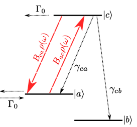
Figure 1: (colour online) Simple 3 level system with optical pumping on $|a\rangle\to|c\rangle$ transition. The steady state populations in each state depend upon the decay fractions $\gamma_{ik}$ and the populations of atoms entering and leaving the beam at rate $\Gamma_{0}$.

Atoms drift into and out of the beam at a rate $\Gamma_{0}$, entering with the equilibrium population distribution and leaving with the optically–pumped distribution. This is discussed further in Section II.4.

We consider the absorption from state $|a\rangle$, so that any population excited from $|b\rangle$ is negligible. The rates of change of the state populations are therefore

$$\frac{\text{d}n_{a}}{\text{d}t} = -n_{a}(B_{ac}\rho(\omega,v)+\Gamma_{0})$$ (17)

$$+n_{c}(B_{ca}\rho(\omega,v)+\gamma_{ca})+\mathcal{N}_{a}\Gamma_{0}$$

$$\frac{\text{d}n_{b}}{\text{d}t} = \Gamma_{0}(-n_{b}+\mathcal{N}_{b})+n_{c}\gamma_{cb}$$ (18)

$$\frac{\text{d}n_{c}}{\text{d}t} = n_{a}B_{ac}\rho(\omega,v)$$ (19)

$$-n_{c}(B_{ca}\rho(\omega,v)+\gamma_{c}+\Gamma_{0}),$$

where $\mathcal{N}_{a}$ and $\mathcal{N}_{b}$ are the fractional equilibrium populations of states $|a\rangle$ and $|b\rangle$, respectively, when $B_{ac}=0$.

The equilibrium populations depend upon the thermal distribution of energies Corney (1987); Demtroder (2003), but for most atoms the ground state splitting is of the order GHz, while the excited state is separated by hundreds of THz from the ground state. The mean energy per degree of freedom is $\frac{1}{2}k_{B}T$, which at room temperature corresponds to a frequency of THz and so we may assume the ground states to be equally populated and the excited state population to be negligible. The equilibrium population of state $|a\rangle$ is therefore

$$\mathcal{N}_{a}=\frac{g_{a}}{g_{a}+g_{b}}N_{V}.$$ (20)

When the rate of the laser scanning across the resonance is much slower than any depopulation mechanisms in the system, we may assume that the populations have reached their steady state values ($\dot{n}_{a}=\dot{n}_{b}=\dot{n}_{c}=0$) and hence become

$$n_{a} = \frac{n_{c}\left(B_{ca}\rho(\omega,v)+\gamma_{ca}\right)+\mathcal{N}_{a}\Gamma_{0}}{B_{ac}\rho(\omega,v)+\Gamma_{0}},$$ (21)

$$n_{c} = \frac{n_{a}B_{ac}\rho(\omega,v)}{\gamma_{c}+\Gamma_{0}+B_{ca}\rho(\omega,v)},$$ (22)

where we assume $|\omega-\omega_{ca}|\ll|\omega-\omega_{cb}|$ and hence may neglect $n_{b}$. This makes the derivation valid for any open two-level system. We then substitute Equation 22 into 21 and rearrange to find $n_{a}$,

$$n_{a}=\frac{\mathcal{N}_{a}}{1+\frac{g_{c}}{g_{a}}\beta_{ac}\alpha_{ac}}$$ (23)

where

$$\alpha_{ac}=\left(1+\frac{\gamma_{c}+\Gamma_{0}}{B_{ca}\rho(\omega,v)}\right)^{-1}$$ (24)

is the saturation parameter, and

$$\beta_{ac}=1+\frac{\gamma_{c}-\gamma_{ca}}{\Gamma_{0}}$$ (25)

is the optical pumping parameter which enhances the saturation of the spectra. As derived in Section II.1, the absorption cross section for the incident beam is proportional to the population difference between the ground and excited states, $B_{ac}n_{a}-B_{ca}n_{c}$ which we may find in terms of $\mathcal{N}_{a}$ by using equation 22

$$B_{ac}n_{a}-B_{ca}n_{c} = B_{ac}\mathcal{N}_{a}\left(\frac{1-\alpha_{ac}}{1+\frac{g_{c}}{g_{a}}\beta_{ac}\alpha_{ac}}\right)$$ (26)

$$= B_{ac}\mathcal{N}_{a}\Delta N$$

where $\Delta N$ is the population difference caused by the pump beams. This may be rearranged into a form similar to Equation 13

$$\Delta N=\left(\frac{1-\alpha_{ac}}{1+\frac{g_{c}}{g_{a}}\beta_{ac}\alpha_{ac}}\right)=\left[1+\frac{I_{P}}{2I^{R}_{ac}}L(\omega,-v)\right]^{-1},$$ (27)

in which $I^{R}_{ac}$ is the reduced saturation intensity reported in the literature Pappas et al. (1980); Demtroder (2003) which is valid for an open two level system:

$$I_{ik}^{R}=I_{ik}\left(\frac{1+\Gamma_{0}/\gamma_{k}}{2+(\gamma_{k}-\gamma_{ki})/\Gamma_{0}}\right).$$ (28)

The numerator in the first term of Equation 27 accounts for the steady state population pumped into the excited states and the denominator accounts for the population pumped into the ground states.

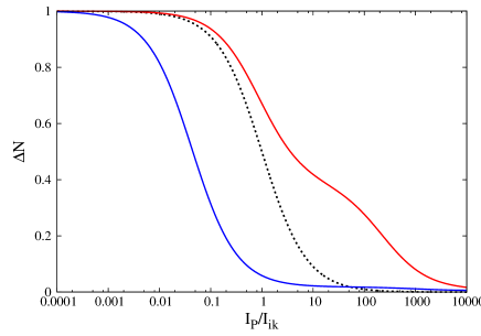
Figure 2: (colour online) The effect of optical pumping in multilevel atoms. The dashed line shows the population difference using Equation 27, i.e., no optical pumping. The solid blue line shows the population difference for the ⁸⁵Rb $F=3\to F^{\prime}=3$ transition in which optical pumping significantly empties the upper ground state at intensities much lower than saturation. The solid red line shows the population difference for the ⁸⁵Rb $F=3\to F^{\prime}=4$ transition which is normally considered ‘closed’; we would expect the population to follow the dashed line and equal $1/2$ at the saturation intensity. In the absence of off-resonant pumping the population will tend toward an equilibrium with the transit rate $\Gamma_{0}$ ($\Delta N\sim 0.44$ in this instance) and so the population at saturation would equal one half of this value from unity ($1-\frac{1}{2}0.44=0.72$). The equilibrium value is not reached at high intensities due to increased off resonant optical pumping, but evidence for this can be seen in the slight shoulder around $I_{P}/I_{ik}=100$.

II.3 Multilevel atoms

Equation 26 may be intuitively extended to include multiple ground ($i$) and excited ($k$) levels.

$$\Delta N(v) = \sum_{i}\Delta N_{i}(v)=\sum_{i}\mathcal{N}_{i}\frac{1-\alpha_{ik}(v)}{1+\frac{g_{k}}{g_{i}}\beta_{ik}\alpha_{ik}(v)}$$ (29)

$$\alpha_{ik}(v) = \sum_{k}\left(1+\frac{\gamma_{j}+\Gamma_{0}}{B^{P}_{ki}\rho(\omega,v)(\omega,v)}\right)^{-1}$$ (30)

$$\beta_{ik} = \sum_{k}1+\frac{\gamma_{k}-\gamma_{ki}}{\Gamma_{0}}.$$ (31)

The absorption of the probe beam is therefore

$$\frac{\text{d}I(\omega)}{\text{d}z}=-\frac{\hbar\gamma}{2\pi c}N_{V}\int_{-\infty}^{+\infty}f_{D}(v)\Delta N(-v)\sum_{i,k}B^{0}_{ik}\rho(\omega,v)\text{d}v.$$ (32)

Because of optical pumping even at low intensities, the pump beam can no longer be assumed to have a negligible effect upon the spectra. Therefore, the pumping rates in the above model are given by

$$B^{P}_{ki}\rho(\omega,v)=\frac{\gamma^{2}}{8cg_{i}}\Bigg{(}\frac{I_{P}}{I_{ik}}\frac{\gamma/2}{(\omega-\omega_{ik}-kv)^{2}+(\frac{\gamma}{2})^{2}}$$

$$+\frac{I_{0}}{I_{ik}}\frac{\gamma/2}{(\omega-\omega_{ik}+kv)^{2}+(\frac{\gamma}{2})^{2}}\Bigg{)}$$ (33)

and

$$B^{0}_{ik}\rho(\omega,v)=\frac{\gamma^{2}}{8cg_{i}}\Bigg{(}\frac{I_{0}}{I_{ik}}\frac{\gamma/2}{(\omega-\omega_{ik}+kv)^{2}+(\frac{\gamma}{2})^{2}}\Bigg{)}.$$ (34)

Note that for Equation 33 the Doppler shift for the probe beam is opposite to that of the pump beam.

This model may be simplified by considering the steady state population for open or closed transitions with fast (MHz) decay rates. Off-resonant pumping into the dark state must be included both to model crossover peaks correctly Demtroder (2003) and because an equilibrium is set up between pumping and transit of atoms into the beam (see Figure 2). For an open transition the atoms will be pumped into the dark state before a significant population builds up in the excited state, so one may use the following form

$$\Delta N=\left(1+\sum_{k}\frac{g_{k}}{g_{i}}\alpha_{ik}\beta_{ik}\right)^{-1}.$$ (35)

For a closed state (such as ⁸⁵Rb $F=3\to F^{\prime}=4$) a significant population will build up in the excited state, but the off-resonant excited state populations will be negligible. In such a situation off-resonant optical pumping into the dark ground states reduces the equilibrium population as shown in Figure 2 and Equation 29 may then be simplified to the form

$$\Delta N=\frac{1-\alpha_{ik}}{1+\sum_{k}\frac{g_{k}}{g_{i}}\alpha_{ik}\beta_{ik}}.$$ (36)

II.4 Transit broadening

Transit broadening is normally considered in the context of a limit to the interaction time and hence to the fundamental resolution of the spectra. For a Gaussian laser beam with a $1/e^{2}$ radius $R$ passing through a dilute gas of atoms with a mean velocity $u$, the standard result (1976) (ed.); Demtroder (2003) for the transit rate of an atom through the beam is

$$\Gamma_{0}=\frac{2u\sqrt{\ln 2}}{R}.$$ (37)

However, we can see in Equation 25 that the transit rate has a significant effect on the optical pumping rate. It is common practice to use large beams to reduce the transit broadening but this has the effect of increasing the time during which atoms may be optically pumped into the dark state, and hence acts to decrease the resolution. In Figure 2 we see that optical pumping occurs at intensities much lower than $I_{ik}$; in fact, the atom can be pumped into the dark state $|b\rangle$ with the absorption of a single photon and so this complicates the calculation of the beam width. If we assume that significant optical pumping occurs at a specific intensity, $I_{\varphi}$, and calculate the width of beam at this intensity as the total pump intensity is changed, the transit rate becomes;

$$\Gamma_{ik}=\left\{\begin{array}[]{cr}\Gamma_{0}\left[\sqrt{\frac{1}{2}\ln\left(\frac{I_{P}}{I_{\varphi}}\right)}\right]^{-1}&\text{if }I_{P}>I_{\varphi}\\ \Gamma_{0}&\text{if }I_{P}\leq I_{\varphi}\end{array}\right.$$ (38)

The transit rate here depends upon the specific transition ($i\to k$), since the apparent increase of beam width will depend upon the individual transition strength. It is not obvious what value of $I_{\varphi}$ of should be used; however in the following model we find empirically that the reduced saturation intensity ($I_{\varphi}=I^{R}_{ik}$) fits the data well.

II.5 Additional broadening mechanisms

The experimental setup may introduce extra broadening of the spectral features and although they are usually much less than the natural and Doppler linewidths, they can be on the order of the transit rate.

The following broadening mechanisms have a Lorentzian lineshape or effect the frequency detuning, therefore may be included to our model by summation with the natural decay rate Corney (1987).

II.5.1 Laser linewidth

As mentioned earlier, the resolution of the spectral features is constrained by the tool we use to measure them: the laser. Diode lasers are a common tool for pump probe spectroscopy and may have linewidths down to the hundreds of kHz region with the addition of an external cavity. We assume a Lorentzian spectral laser line-shape with a full width at half maximum (FWHM) $\Gamma_{L}$ in angular frequency units.

II.5.2 Geometrical broadening

The sub-Doppler resolution depends upon atoms traversing the beams at a perpendicular angle. Therefore, if the beams are not exactly anti-parallel they will sample a non-zero atomic velocity component and hence decrease the resolution. In the experimental arrangement described in Section IV, perfect beam overlap is achieved using a polarizing beam–splitting cube. For some experiments the polarizations of each beam may need to be controlled independently, and back-reflections into the laser cavity may be unwanted, favoring a geometry in which the counter-propagating beams cross at a non-zero angle $\theta$. This results in a broadening (1976) (ed.)

$$\Gamma_{G}=(\vec{k}_{P}-\vec{k}_{0})\cdot\vec{v}=\frac{2u\omega_{ik}}{c}\,\sin(\tfrac{1}{2}\theta).$$ (39)

where $\vec{k}_{P}$ and $\vec{k}_{0}$ are the pump and probe wavevectors, respectively.

II.5.3 Beam collimation

An uncollimated beam passing through the vapor cell will result in a variation of transit time along the cell. Wavefront curvature also broadens the Lamb dip in much the same manner as geometrical broadening. To limit this effect the radius of curvature of the wavefronts must be much greater than $kR^{2}/4$ Letokhov and Chebotayev (1977).

II.5.4 Collisional broadening

We have limited our model to dilute gases in which collisions during the interaction time are negligible. In dense gases the collisional cross-section can be as large as the absorption cross-section and can affect the spectra by broadening and shifting the peak. Collisions may also affect the distribution of population amongst the ground states. The magnitude and nature of the effect depend upon density, temperature and collisional partners (i.e., non-identical atoms in the case of a buffer gas) Corney (1987).

III Rubidium

Natural rubidium occurs in two stable isotopes, ⁸⁵Rb and ⁸⁷Rb, with fractional abundances, $f_{I}$, of 0.2783 and 0.7217, and atomic masses 84.912 and 86.909, respectively Lide (2001-2002). The ground state is $5S_{1/2}$, with nuclear moment $I=5/2$ for ⁸⁵Rb and $I=3/2$ for ⁸⁷Rb, and orbital angular momentum $L=0$ and spin $S=1/2$. The excited state under investigation is $5P_{3/2}$ state with $L=1$ and the transition between these states is known as the $D_{2}$ line. Due to the non-zero nuclear angular momentum each state is split into $2J+1$ hyperfine levels, each of which has $2(2I+1)$ magnetic sublevels. Figure 3 shows the hyperfine structure of both isotopes and the energy splitting between levels. The Clebsch-Gordan coefficients, saturation intensity (Equation 14) and fractional decay rates $\gamma_{ik}$ used in the model are shown in Table 1. The natural lifetime is $26.25\pm 0.07\thinspace$ns Schultz et al. (2008) for both isotopes.

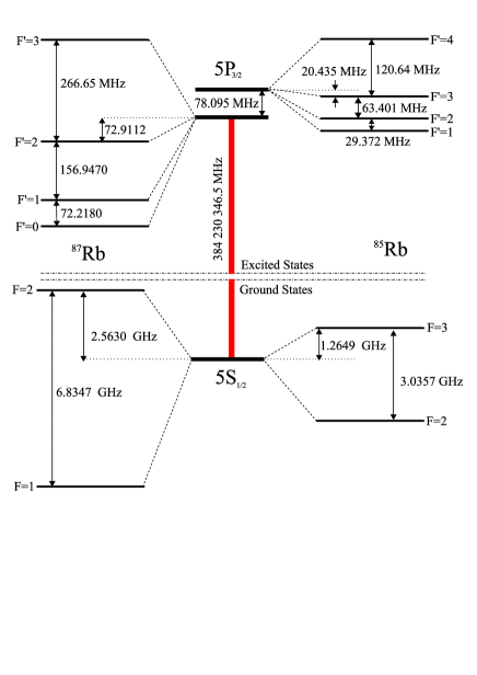
Figure 3: Hyperfine structure of ⁸⁵Rb and ⁸⁷Rb.

	$F_{i}$	$F_{k}$	$I_{ik}$(mW cm-2)	$C^{2}_{ik}$	$\gamma_{ki}(\gamma)$
85Rb	3	4	3.894	1	1
	3	3	9.012	35/81	$5/9$
	3	2	31.542	10/81	$2/9$
	2	3	8.046	28/81	$4/9$
	2	2	6.437	35/81	$7/9$
	2	1	8.344	1/3
87Rb	2	3	3.576	7/9	$1$
	2	2	10.013	5/18	$1/2$
	2	1	50.067	1/18	$1/6$
	1	2	6.008	5/18	$1/2$
	1	1	6.008	5/18	$5/6$
	1	0	15.020	1/9	$1$

Table 1: Rubidium model parameters for linear polarization and degenerate hyperfine levels.

Rubidium has a melting point of 39.3℃and the number density is then given by Nesmeyanov (1963)

$$N_{V}=\frac{f_{I}}{k_{B}T}133.323\times 10^{p_{j}}\\$$ (40)

where the exponent subscript $j=S,L$ corresponds to solid and liquid rubidium, respectively, with

$$p_{S} = -94.04826-\frac{1961.258}{T}$$ (41)

$$-0.03771678\times T+42.57526\ln(T)$$

$$p_{L} = 15.88253-\frac{4529.535}{T}$$ (42)

$$+0.00058663\times T-2.99138\ln(T).$$

IV Pump–Probe Apparatus

We have tested our model experimentally with rubidium vapor in a pump-probe apparatus, normally used to stabilize diode lasers for a magneto-optical trap, shown in Figure 4. The diode laser had an external cavity in the Littrow configuration with a beam diameter of $2.1\pm 0.1$ mm in the vertical plane. The beam was elliptical with a horizontal width equal to twice the height; the greatest transit broadening thus results from the narrower dimension and the model therefore uses the above value. The beams were overlapped through the vapor cell by sending the pump beam through a polarizing beam splitter cube (PBSC); the counterpropagating probe beam had a linear polarization perpendicular to the pump beam and was reflected by the PBSC onto the photodiode. This layout allowed perfect overlap of the beams and a reduced footprint of the apparatus.

The laser frequency was scanned via rotation of the external cavity grating with a piezoelectric transducer and spectra were averaged over three scans. The scans were not linear, so the frequency axis was calibrated using the 12 resonance and crossover peaks (see Figure 3) by fitting to a fourth-order polynomial; the standard deviation of the fitted peaks from tabulated values was $<400$ kHz. The probe power was kept at $1\mu$W and the laser linewidth was $1.0\pm 0.2$ MHz [28]. The vapor cell had length of 75 mm and a temperature of $18.0\pm 0.1$ ℃. No attempt was made to null the Earth’s or nearby magnetic fields.

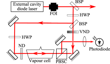
Figure 4: The pump–probe spectroscopy apparatus used for the spectra in Section V. Approximately 3 mW is picked off from the external cavity diode laser (ECDL) with a beam–splitter plate (BSP). The ECDL is protected from back reflection by a Faraday Optical Isolator (FOI), so that the beam may be perfectly overlapped using a polarizing beam splitter cube (PBSC). The linear polarization of the probe (left to right through the vapor cell) and pump (right to left) beams are rotated by half waveplates (HWP) so that the pump is transmitted and the probe reflected by the PBSC. The power of the pump beam is controlled with a variable neutral density filter (VND).

V Comparison between Experiment and Theory

The experimentally measured pump probe spectra for the upper ground states of ⁸⁵Rb and ⁸⁷Rb are shown together with predictions of the theoretical model in Figure 6$i$, where $i$=$a$,$b$,$c$,$d$ relate to the pump powers 20$\,\mu$W, 100$\,\mu$W, 500$\,\mu$W and 2500$\,\mu$W, respectively. Figure 6 is split into four parts: plots $i$-3 shows the full absorption spectrum with the experimental data in black and the theoretical curves in red, plots $i$-1,2 show a magnified sections of the Lamb dips ($i$-1=⁸⁷Rb, $i$-2=⁸⁵Rb) and plots $i$-4 shows the experimental data subtracted from the theoretical curves (residuals).

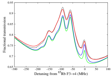
Figure 5: (colour online) The effect of beam width on sub-Doppler features. The dashed line and solid red line correspond to the Figure 6d-2. The blue line shows the same model but without the additional beam broadening factor from Equation 38. The green line includes the additional broadening factor but assumes a $1/e^{2}$ beam width twice that in the red plot. The laser power remains the same for each plot.

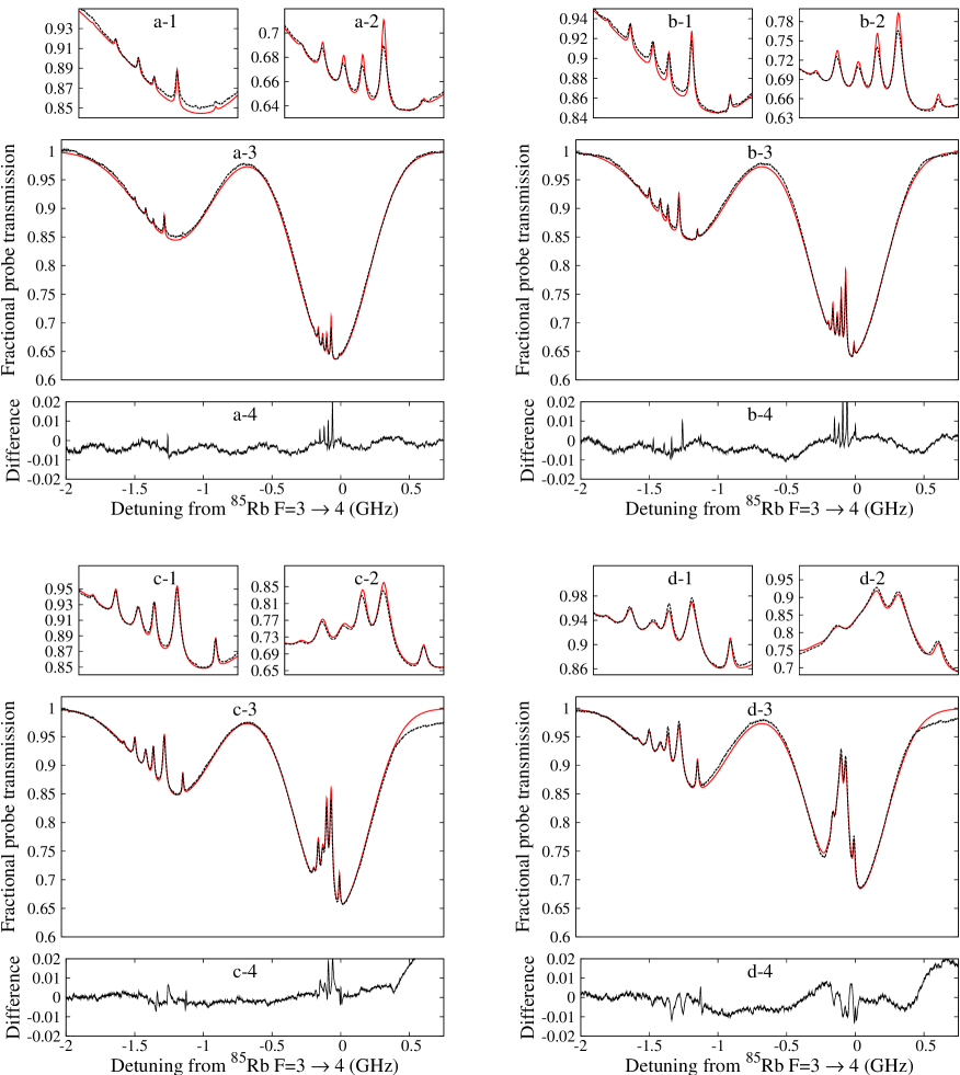
Figure 6: Normalized pump probe transmission spectra of ⁸⁵Rb $F=3\to 4$ (right hand dip) and ⁸⁷Rb $F=2\to 3$ (left-hand dip) for pump powers of 20$\,\mu$W, 100$\,\mu$W, 500$\,\mu$W and 2500$\,\mu$W, relating to a,b,c,d respectively. The experimental data are shown by black dashes and the theoretical curves by the solid red line. Plots i-1,2 are magnified sections of the full absorption spectra i-3, and i-4 is the difference between the data and model. The large deviations in Figures c,d-3,4 above +0.5 GHz are due to the nonlinear scanning of the piezo near a turning point.

It is apparent that our theoretical model accurately predicts the height and width of each absorption line. The residuals have a standard deviation of less than 1%, and much of this is due to experimental noise and calibration errors. In Figures 6a-4 and 6b-4, the noise is dominated by a sinusoidal signal from power line pickup.

Our model appears to slightly overestimate the height of the Lamb dips at low powers. This may be due to errors in the beam power measurement or the elliptical cross section of the laser beams. This latter point complicates the effect of beam width on optical pumping, and the arbitrary value used for $I_{\varphi}$ in Section II.4. The effect of these values is shown in Figure 5.

VI Conclusion

A simple model of pump–probe spectroscopy based on the rate equations has been presented and compared against the experimental spectrum of rubidium. Our model can describe multilevel atoms and fits the data well with the residual difference less than 1% over a large range of pump powers. The model is valid for any dilute gas when coherent effects are negligible, and accounts for finite laser linewidth, optical pumping and transit time broadening.

The most significant effect upon the spectral features is the optical pumping during the atom’s transit across the beam. As opposed to saturation broadening, which is due to the equalization of populations in the ground and excited states preventing further absorption, optical pumping can transfer population into dark states, which also prevents further absorption but may occur for a single photon absorption. The time taken by the atom to transverse the beam significantly affects the optical pumping and therefore careful attention must be made in defining the beam width.