Backaction of a charge detector on a double quantum dot

Abstract

We develop a master equation approach to study the backaction of quantum point contact (QPC) on a double quantum dot (DQD) at zero bias voltage. We reveal why electrons can pass through the zero-bias DQD only when the bias voltage across the QPC exceeds a threshold value determined by the eigenstate energy difference of the DQD. This derived excitation condition agrees well with experiments on QPC-induced inelastic electron tunneling through a DQD [S. Gustavsson et al., Phys. Rev. Lett. 99, 206804(2007)]. Moreover, we propose a scheme to generate a pure spin current by the QPC in the absence of a charge current.

I Introduction

Recent technological advances have made it possible to confine, manipulate, and measure a small number of electrons or just one electron in a single or double quantum dot (DQD).ElzermanNature04 ; PettaPRL04 ; DiCarloPRL04 ; HayashiPRL03 In most experiments, the electron occupancy in a quantum dot is usually measured by a local quantum point contact (QPC) charge detector.FieldPRL93 ; ElzermanPRB03 In such a system, the backaction of the charge detector to the DQD is of particular interest.

Several previous theoretical works (see e.g., Refs. GoanPRB01, ; GurvitzPRB97, ; Ouyang06, ) involving this coupled DQD-QPC system mainly focus on the QPC-induced decoherence of the electronic states in the DQD. Recently, the impacts of the backaction on the electron transport through a zero-bias DQD were experimentally investigated.Gustavsson07 ; Gasser09 It is suggested that the QPC emits photons which can be absorbed by a nearby zero-bias DQD. The photon absorption process at the same time induces the interdot electronic transitions inside the DQD and then changes the DQD occupancy, which can be measured by the QPC. These works show how strong the backaction of a detector on a qubit is and provide an efficient solid state implementation for the detection of a single photon. More importantly, the experiments show that these interdot transitions can only be driven when the energy $|eV_{d}|$ (with $e$ the charge unit and $V_{d}$ the bias voltage across the QPC) emitted by the QPC exceeds the eigenenergy difference $\Delta$ of the DQD, rather than the energy difference $\varepsilon$ of the local orbital levels in the two dots [see Fig. 1(b)]. This means that, if $|eV_{d}|\leq\Delta$, the interdot transitions cannot be driven. Previously suggested mechanisms based on current fluctuations through the QPC for interpreting the inelastic transition in Ref. Gustavsson07, involve a perturbative approximation Gustavsson07 ; AguadoPRL ; Onac06 which is valid for a weak interdot coupling. An alternative mechanismGasser09 ; Khrapai06 considering the QPC as an effective bosonic bath of the DQD was also proposed to describe the underlying physics. However, how this effective bosonic bath is related to the QPC is not explicitly demonstrated.

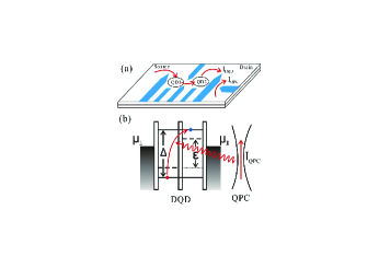
Figure 1: (Color online) (a) Schematic diagram of a DQD connected to two electrodes via tunneling barriers. A QPC used for measuring the electron states yields backaction on the DQD. (b) QPC-driven interdot electronic transition between two DQD eigenstates with an energy difference $\Delta$. The energy detunning $\varepsilon$ between the two single-dot levels (dashed lines) can be varied by tuning the gate voltages.

In this paper, we theoretically analyze the backaction of the QPC on the DQD. Starting from a microscopic description of the whole system, we derive a master equation (ME) based on the eigenstate-basis of the DQD to describe the quantum dynamics of the DQD. Similar eigenstate-basis ME was used by Stace and BarretStacePRL04 to study the QPC-induced decoherence properties of the DQD. We show that this ME approach provides a satisfactory theoretical understanding of the backaction of the QPC on the DQD. In particular, experimental observations of the inelastic electron tunneling through a zero-bias DQD driven by a nearby QPCGustavsson07 ; Gasser09 can be well explained. Moreover, we propose an approach for generating a pure spin current through a DQD. Interestingly, this spin current is driven by the nearby QPC and can occur without a charge current.

This paper is organized as follows. In Sec. II, we model the coupled DQD-QPC system and derive a master equation to describe the quantum dynamics of the DQD in the presence of the charge detector. As shown in Sec. III, this master equation naturally yields the main condition under which the electron in the DQD can be excited by the QPC. In Sec. IV, we show that the current through the DQD can be induced by this QPC even when the DQD is at zero-bias voltage. Specifically, this QPC-induced current is proportional to the capacitive coupling strength between the DQD and the QPC. In Sec. V, based on the same excitation mechanism by a nearby QPC, we propose a scheme to generate a pure spin current through a zero-bias DQD. Finally, we conclude in Sec. VI.

II Characterization of a DQD coupled to a QPC

For a DQD, both intra- and inter-dot Coulomb repulsions play an important role in the Coulomb-blockade effect (see, e.g., Ref. YouPRB, ). Here we consider the regime with strong intra- and inter-dot Coulomb interactions so that only one electron is allowed in the DQD (see Fig. 1). The states of the DQD are denoted by the occupation states $|0\rangle$, $|1\rangle$, and $|2\rangle$, representing respectively an empty DQD, one electron in the left dot, and one electron in the right dot. The total Hamiltonian of the system is given by

$$H_{\rm tot}=H_{\rm DQD}+H_{\rm QPC}+H_{\rm det}+H_{\rm leads}+H_{\rm T},$$ (1)

where (we set $\hbar=1$)

$$H_{\rm DQD}\!=\!\frac{\varepsilon}{2}\sigma_{z}+\Omega\sigma_{x},$$ (2a)

$$H_{\rm QPC}\!=\!\sum_{kq}\omega_{Sk}c_{Sk}^{\dagger}c_{Sk}+\omega_{Dq}c_{Dq}^{\dagger}c_{Dq},$$ (2b)

$$H_{\rm det}\!=\!\sum_{kq}(T-\chi_{1}a_{1}^{\dagger}a_{1}-\chi_{2}a_{2}^{\dagger}a_{2})(c_{Sk}^{\dagger}c_{Dq}+{\rm H.c.}),$$ (2c)

$$H_{\rm leads}\!=\!\sum_{s}\omega_{ls}c_{ls}^{\dagger}c_{ls}+\omega_{rs}c_{rs}^{\dagger}c_{rs},$$ (2d)

$$H_{\rm T}\!=\!\sum_{s}(\Omega_{ls}c_{ls}^{\dagger}a_{1}+\Omega_{rs}\Upsilon_{r}^{\dagger}c_{rs}^{\dagger}a_{2}+{\rm H.c.}).$$ (2e)

Here $H_{\rm DQD}$, $H_{\rm QPC}$, and $H_{\rm leads}$ are the free Hamiltonians of the DQD, the QPC, and the electrodes connected to the DQD respectively. In Eq. (2a), $\varepsilon$ is the energy detuning between the two dots and $\Omega$ is the interdot coupling. $c_{Sk}$ ($c_{Dk}$) is the annihilation operator for electrons in the source (drain) of the QPC with momentum $k$, while $c_{\alpha s}$ is the annihilation operator for electrons in the $\alpha$th ($\alpha=l,r$) electrode. Moreover, $\sigma_{z}=a_{2}^{\dagger}a_{2}-a_{1}^{\dagger}a_{1}$ and $\sigma_{x}=a_{2}^{\dagger}a_{1}+a_{1}^{\dagger}a_{2}$ are Pauli matrices, with $a_{1}$ ($a_{2}$) the annihilation operator for electrons staying at the left (right) dot. $H_{\rm det}$ describes the electrostatic DQD-QPC coupling, in which $T$ is the tunneling amplitude of an isolated QPC and $\chi_{1}$ ($\chi_{2}$) gives the variation of the tunneling amplitude when the extra electron stays at the left (right) dot. Usually one has $\chi_{1}<\chi_{2}$ since the QPC is located more closely to the right dot. Furthermore, $H_{\rm T}$ gives the tunneling couplings of the DQD to the two electrodes and it depends on the tunneling coupling strengths $\Omega_{lk}$ and $\Omega_{rk}$. In Eq. (2e), we have also introdued the operators $\Upsilon_{r}$, $\Upsilon_{r}^{\dagger}$ to count the number of electrons that have tunneled into the right lead.ME-E

First, we diagonize the Hamiltonian of the DQD as

$$H_{\rm DQD}=\frac{\Delta}{2}(|e\rangle\langle e|-|g\rangle\langle g|)=\frac{\Delta}{2}\sigma_{z}^{(e)},$$ (3)

where $\Delta=\sqrt{\varepsilon^{2}+4\Omega^{2}}$ is the energy splitting of the two eigenstates of the DQD given by $|g\rangle=\alpha|1\rangle-\beta|2\rangle$, and $|e\rangle=\beta|1\rangle+\alpha|2\rangle$, with $\alpha\equiv\cos{\theta}/{2}$, $\beta\equiv\sin{\theta}/{2}$, and $\tan\theta=2\Omega/\varepsilon$. This eigenstate basis will be adopted in all the following calculations. To describe the dynamics of the system, we derive the ME starting from the von Neumann equation

$$\dot{\rho}_{R}(t)=-i[H_{\rm tot},\,\rho_{R}],$$ (4)

with $\rho_{R}$ the density matrix of the whole system. In the interaction picture defined by the free Hamiltonian

$$H_{0}=H_{\rm DQD}+H_{\rm QPC}+H_{\rm leads},$$ (5)

the interaction Hamiltonian $H_{\rm I}=H_{\rm det}+H_{\rm T}$ is given by

$$H_{\rm I}(t)=A(t)Y(t)+H_{\rm T}(t),$$ (6)

where

$$A(t)\! =\!\sum_{n=1}^{3}P_{n}e^{-i\omega_{n}t},$$ (7a)

$$Y(t)\! =\!\sum_{kq}[c_{Sk}^{\dagger}c_{Dq}e^{i(\omega_{Sk}-\omega_{Dq})t}+{\rm H.c.}],$$ (7b)

$$H_{\rm T}(t)\! =\!\sum_{s}\big{[}c_{ls}^{\dagger}(\alpha a_{g}e^{-i\Delta t/2}+\beta a_{e}e^{i\Delta t/2})e^{i\omega_{ls}t}+\Upsilon_{r}^{\dagger}c_{rs}^{\dagger}$$

$$\times(-\beta a_{g}e^{-i\Delta t/2t}+\alpha a_{e}e^{i\Delta t/2})e^{i\omega_{rs}t}+{\rm H.c.}\big{]}.$$ (7c)

In Eq. (7a), we have defined

$$P_{1}=-\alpha\beta|e\rangle\langle g|,~{}~{}P_{2}=-\alpha\beta|g\rangle\langle e|,$$

$$P_{3}=T-(\chi_{1}|e\rangle\langle e|+\chi_{2}|g\rangle\langle g|)+\alpha^{2}\chi_{d}\sigma_{z}^{(e)},$$ (8)

with $\chi_{d}=\chi_{1}-\chi_{2}$. Also, we have chosen $\omega_{1}=-\omega_{2}=-\Delta$, and $\omega_{3}=0$. Integrating the von Neumann equation within the Born-Markov approximation and tracing over the degrees of freedom of the QPC and the two electrodes, one obtainsBlum

$$\dot{\rho}(t)\! \!=\! \!{\rm Tr}_{R}\bigg{(}\!\!-i[H_{\rm I}(t),\rho_{R}(0)]$$ (9)

$$-\!\int\limits_{0}^{t}dt^{\prime}[H_{\rm I}(t),\,[H_{\rm I}(t^{\prime}),\,\rho_{R}(t)]]\bigg{)}.$$

Following the experimental conditions, we consider a zero bias across the DQD. We also set $\mu_{L}=\mu_{R}=0$ [see Fig. 1(b)] although other values of $\mu_{L}$ and $\mu_{R}$ satisfying $\Delta/2\!>\!\mu_{L}\!>\!-\Delta/2$ give identical results . Substituting $H_{\rm I}(t)$ shown in Eqs. (6) and (7) into Eq. (9), neglecting the fast-oscillating terms (which are proportional to $e^{\pm i\Delta t}$), and converting the obtained equation into the Schrödinger picture, we obtain the ME:ME-E

$$\dot{\rho}(t)\!=\!-i[H_{\rm DQD},\,\rho(t)]+\mathcal{L}_{d}\rho(t)+\mathcal{L}_{T}\rho(t)+\gamma\mathcal{D}[a_{g}^{\dagger}a_{e}]\rho,$$

(10)

with

$$\mathcal{L}_{d}\rho(t)\! \!=\! \!2\pi g_{S}g_{D}\sum_{i=1}^{3}\big{\{}\mathcal{D}[P_{i}]\rho(t)\Theta(eV_{d}+\omega_{i})$$

$$+\mathcal{D}[P_{i}^{\dagger}]\rho(t)\Theta(-eV_{d}-\omega_{i})\big{\}},$$

$$\mathcal{L}_{T}\rho(t)\! \!=\! \!\Gamma_{L}\alpha^{2}\mathcal{D}[a_{g}^{\dagger}]\rho+\Gamma_{L}\beta^{2}\mathcal{D}[a_{e}]\rho$$ (11)

$$+\Gamma_{R}\beta^{2}\mathcal{D}[a_{g}^{\dagger}\Upsilon_{r}]\rho+\Gamma_{R}\alpha^{2}\mathcal{D}[a_{e}\Upsilon_{r}^{\dagger}]\rho.$$

The notation $\mathcal{D}$ acting on any operator $A$ is defined by

$$\mathcal{D}[A]\rho=A\rho A^{\dagger}-\frac{1}{2}(A^{\dagger}A\rho+\rho A^{\dagger}A).$$ (12)

Also, $\Gamma_{L(R)}=2\pi g_{L(R)}\Omega_{lk(rk)}^{2}$ is the rate for electron tunneling through the left (right) barrier and $\Theta(x)=(x+|x|)/2$. $g_{i}$ ($i=S$,$D$,$L$, or $R$) denotes the density of states at the QPC source, the QPC drain, the left DQD electrode, or the right DQD electrode, which is assumed to be constant over the relevant energy range. Furthermore, to allow for the couplings of the DQD to other degrees of freedom, such as hyperfine interactions and electron-phonon couplings, we phenomenologically include an additional relaxation term [the fourth term in Eq. (10)] describing transitions from the excited state $|e\rangle$ to the ground state $|g\rangle$.

III QPC-induced excitation condition

Below we use the ME to derive the electron tunneling rates into and out of the DQD at zero bias voltage. From Eqs. (10) and (11) and the relations

$$\langle n|\Upsilon_{r}^{\dagger}\Upsilon_{r}\rho|n\rangle=\rho^{(n)},~{}\langle n|\Upsilon_{r}\Upsilon_{r}^{\dagger}\rho|n\rangle=\rho^{(n)},$$

$$\langle n|\Upsilon_{r}^{\dagger}\rho\Upsilon_{r}|n\rangle=\rho^{(n-1)},~{}\langle n|\Upsilon_{r}\rho\Upsilon_{r}^{\dagger}|n\rangle=\rho^{(n+1)},$$ (13)

we obtain the $n$-resolved equation of motion for each reduced density matrix element:

$$\dot{\rho}_{00}^{(n)}\! =\! -\Gamma_{1}\rho_{00}^{(n)}+\Gamma_{L}\beta^{2}\rho_{ee}^{(n)}+\Gamma_{R}\alpha^{2}\rho_{ee}^{(n-1)},$$

$$\dot{\rho}_{gg}^{(n)}\! =\! \Gamma_{L}\alpha^{2}\rho_{00}^{(n)}+\Gamma_{R}\beta^{2}\rho_{00}^{(n+1)}-\Gamma_{a}\rho_{gg}^{(n)}+(\Gamma_{e}+\gamma)\rho_{ee}^{(n)},$$

$$\dot{\rho}_{ee}^{(n)}\! =\! -\Gamma_{2}\rho_{ee}^{(n)}+\Gamma_{a}\rho_{gg}^{(n)}-(\Gamma_{e}+\gamma)\rho_{ee}^{(n)},$$ (14)

where $n$ is the number of electrons that have tunneled through the DQD via the right tunneling barrier at time $t$, so that $\rho_{ij}=\sum_{n}\rho_{ij}^{(n)}$ $(i,j\!=\!0,g,e)$. In Eq. (14), we have defined the QPC-induced excitation and relaxation rates:

$$\Gamma_{a,e}=2\pi g_{S}g_{D}\chi_{d}^{2}(\alpha\beta)^{2}[\Theta(eV_{d}\mp\Delta)+\Theta(-eV_{d}\mp\Delta)].$$ (15)

as well as the tunneling rates $\Gamma_{1}=\Gamma_{L}\alpha^{2}+\Gamma_{R}\beta^{2}$, and $\Gamma_{2}=\Gamma_{L}\beta^{2}+\Gamma_{R}\alpha^{2}$.

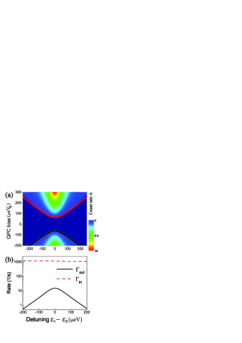
Figure 2: (Color online) (a) Tunneling rate $\Gamma_{\rm out}$ as a function of both the energy detuning $\varepsilon_{1}-\varepsilon_{2}$ and the QPC bias voltage $V_{d}$. The hyperbolic curves mark the two eigenenergy levels of the DQD. (b) Tunneling rates $\Gamma_{\rm in}$ and $\Gamma_{\rm out}$ versus the energy detuning. We use the typical experimental parameters in Ref. Gustavsson07, : $V_{d}=-300~{}\mu$eV, $\Omega=32~{}\mu$eV, $\Gamma_{L}=1.2$ kHz, $\Gamma_{R}=1.1$ kHz, $T=0.5$, $\chi_{1}=0.028~{}T$, $\chi_{2}=0.05~{}T$, and $1/\gamma=2$ ns.

The environment-induced relaxation ratePettaPRL04 $\gamma$ ($\!\sim\!1~{}$ns) of a DQD is typically much larger than the available measurement bandwith of the QPC, so that transitions between the ground state $|g\rangle$ and the excited state $|e\rangle$ cannot be directly registered by the detector. However, using time-resolved charge-detection techniques, one can measure whether the DQD is occupied by an extra electron or not, so that the measured time traces show two levels.Gustavsson07 From these traces, one can extract the rates of electrons tunneling into and out of the DQD, i.e., $\Gamma_{\rm in}=1/\langle\tau_{in}\rangle$ and $\Gamma_{\rm out}=1/\langle\tau_{out}\rangle$ with $\tau_{in}$ and $\tau_{out}$ being the waiting times for the corresponding tunneling events. At steady state with $\dot{\rho}_{ij}(t\rightarrow\infty)=0$, the number of electrons coming from the left lead to the DQD should be equal to the number of electrons going out of the DQD to the right lead. Thus, one has the equilibrium relation:

$$\Gamma_{\rm in}\rho_{00}=\Gamma_{\rm out}(\rho_{gg}+\rho_{ee}).$$ (16)

For an initially empty DQD, $|0\rangle$, the first term of the first equation in Eq. (III) implies that $\Gamma_{\rm in}=\Gamma_{1}$. Using also the steady state solution of Eq. (14), straightforward algebra gives

$$\Gamma_{\rm out}\!=\!\frac{\Gamma_{a}\Gamma_{2}}{\Gamma_{2}+\Gamma_{e}+\gamma}.$$ (17)

As expected, the rate for electrons tunneling out of the DQD is proportional to the QPC-induced excitation rate $\Gamma_{a}$. Using $\Gamma_{a}$ obtained above, it follows from Eq. (17) that

$$\Gamma_{\rm out}\! \!=\! \!\frac{2\pi g_{S}g_{D}\chi_{d}^{2}(\alpha\beta)^{2}\Gamma_{2}[\Theta(eV_{d}-\Delta)+\Theta(-eV_{d}-\Delta)]}{\Gamma_{2}+\Gamma_{e}+\gamma}.$$

We emphasize that this excitation process occurs (i.e., $\Gamma_{\rm out}>0$) only when the energy emitted by the QPC is larger than the eigenenergy difference of the DQD, i.e.,

$$|eV_{d}|>\Delta.$$ (19)

Otherwise, if $|eV_{d}|\leq\Delta$, $\Gamma_{\rm out}$ is always zero and no excitation process happens. This agrees well with the experiment in Ref. Gustavsson07, . More importantly, we note from Eq. (LABEL:Fout) that

$$\Gamma_{\rm out}\propto\chi_{d}^{2}=(\chi_{1}-\chi_{2})^{2},$$ (20)

which clearly implies that the QPC-induced excitation results from the electrostatic coupling between the DQD and the QPC. Figure 2(a) plots the rate $\Gamma_{\rm out}$ as a function of both the QPC-bias voltage $V_{d}$ and the energy detunning $\varepsilon_{1}-\varepsilon_{2}$ of the DQD. Figure 2(b) gives the calculated rates for electrons tunneling into and out of the DQD as a function of the energy detunning. For almost symmetric tunneling couplings, i.e., $\Gamma_{L}\simeq\Gamma_{R}$, the rate $\Gamma_{\rm in}$ is almost constant and $\Gamma_{\rm out}$ depends strongly on the energy detunning.

IV QPC-driven charge current through the DQD

Without a nearby QPC, an electron can enter the empty zero-bias DQD, but should be trapped by the DQD. This leads to zero current through the DQD. However, the QPC can induce an excitation from the ground state $|g\rangle$ to the excited state $|e\rangle$ [Fig. 1(b)], from which the electron leaves the DQD. When this cycle repeats, a finite current flows through the DQD. Below we study this QPC-induced charge current when the couplings between the DQD and the two electrodes are strongly asymmetric, i.e., $\Gamma_{L}\gg\Gamma_{R}$, as investigated by Gasser et al..Gasser09 The charge current $I_{c}(t)$ through the DQD at time $t$ is

$$I_{c}(t)=e\frac{dN(t)}{dt}=e\sum_{n,i}n\dot{\rho}_{ii}^{(n)},$$ (21)

where $N(t)$ is the number of electrons that have tunneled into the right lead. From Eq. (14), we get

$$I_{c}(t)=e\Gamma_{R}(\alpha^{2}\rho_{ee}-\beta^{2}\rho_{00}).$$ (22)

At steady state, the current becomes

$$I_{c}=\frac{e\Gamma_{L}\Gamma_{R}\Gamma_{a}(\alpha^{2}-\beta^{2})}{\Gamma_{a}(\Gamma_{L}+\Gamma_{R})+\Gamma_{1}(\Gamma_{e}+\gamma+\Gamma_{2})}.$$ (23)

In Gasser et al.’s experiment, the DQD is coupled to two QPCs, i.e., one QPC is adjacent to the left dot and the other to the right dot. This can be characterized by replacing $H_{\rm QPC}$ and $H_{\rm det}$ in Eqs. (2b) and (2c) by

$$H_{\rm QPC}\! \!=\! \!\sum_{i}H_{\rm QPC}^{i}\!=\!\sum_{kqi}\omega_{Ski}c_{Ski}^{\dagger}c_{Ski}+\omega_{Dqi}c_{Dqi}^{\dagger}c_{Dqi},$$

$$H_{\rm det}\! \!=\! \!\sum_{kqi}(T_{i}-\chi_{1i}a_{1}^{\dagger}a_{1}-\chi_{2i}a_{2}^{\dagger}a_{2})(c_{Ski}^{\dagger}c_{Dqi}+{\rm H.c.}).$$

Here $H_{\rm QPC}^{i}$ is the Hamiltonian of the $i$th ($i=L,R$) QPC and $\chi_{1i}$ ($\chi_{2i}$) gives the variation of the tunneling amplitude of the $i$th QPC when the extra electron stays in the left (right) dot. From Eq. (23), one notes that the charge current is determined by $\chi_{d}^{2}$, which characterizes the coupling strength between the DQD and the QPC.

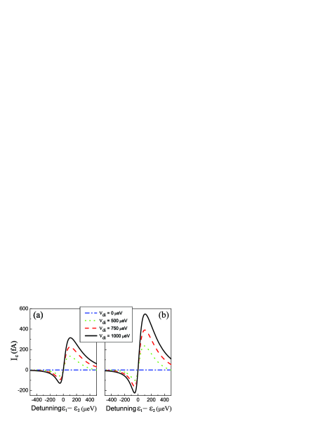
Figure 3: (Color online) QPC-driven static charge current $I_{c}$ through the DQD as a function of the energy detuning for different QPC voltages. (a) $V_{d1}\in[0,1000]~{}\mu$eV, $V_{d2}=0$, and $\chi_{d1}=\chi_{1L}-\chi_{2L}=0.022~{}T_{1}$; (b) $V_{d2}\in[0,1000]~{}\mu$eV, $V_{d1}=0$, and $\chi_{d2}=\chi_{1R}-\chi_{2R}=-0.029~{}T_{2}$. Other parameters are $\Gamma_{L}=0.5~{}$GHz, $\Gamma_{R}=7.8~{}$MHz, $\Omega=35~{}\mu$eV, $T_{1}=T_{2}=0.5$, and $1/\gamma=5~{}$ns.

In Fig. 3, we plot the charge current versus energy detunning for various QPC voltages. Here we choose the current direction from the left to the right to be positive. Comparing Fig. 3(a) with Fig. 3(b), one sees that the current is more pronounced for a larger value of $\chi_{d}^{2}$. This is because the QPC-induced excitation becomes stronger when $\chi_{d}^{2}$ is larger. Furthermore, the asymmetry of the current with respect to the energy detuning $\varepsilon_{1}-\varepsilon_{2}$ can be explained as follows. When $\varepsilon_{1}>\varepsilon_{2}$, one has $\alpha<\beta$ and electrons tunnel from the right electrode to the left one via the DQD. In contrast, electrons tunnel in the opposite direction when $\varepsilon_{1}<\varepsilon_{2}$. In the latter case, however, a small tunneling rate $\Gamma_{R}$ will partially block the current, which leads to the asymmetry of the current. These features were clearly observed in the experiment.Gasser09

V Novel spin-current generator

Finally, we propose a new scheme to generate a pure spin current through the DQD by applying two different static magnetic fields in the quantum dots. Unequal magnetic fields in the two dots can be realized by placing a Co micromagnet near one dot of the DQD.NeilPRL08 When the eigenstate energy difference $\Delta$ becomes spin dependent, the QPC-driven excitation rate depends on the spin states. A spin-polarized current through the DQD can be generated. Here we consider the case with a static magnetic field $B_{z}$ applied only at the left dot. Generalizing the ME in Eq. (14) to take into account the spin degrees of freedom, the current due to electrons with spin $\sigma$ ($=\uparrow,\downarrow$) is given by

$$I_{\sigma}=\frac{e\Gamma_{L}\Gamma_{R}\Gamma_{a}^{\sigma}\Gamma_{a}^{\bar{\sigma}}\Gamma_{2}^{\bar{\sigma}}(\alpha_{\sigma}^{2}-\beta_{\sigma}^{2})}{M_{\sigma}},$$ (25)

where

$$M_{\sigma}\! = \!\Gamma_{a}^{\sigma}\Gamma_{a}^{\bar{\sigma}}(\Gamma_{2}^{\sigma}\Gamma_{2}^{\bar{\sigma}}+\Gamma_{1}^{\sigma}\Gamma_{2}^{\bar{\sigma}}+\Gamma_{1}^{\bar{\sigma}}\Gamma_{2}^{\sigma})$$ (26)

$$+\sum_{s=\sigma,\bar{\sigma}}\Gamma_{a}^{s}\Gamma_{1}^{\bar{s}}\Gamma_{2}^{s}(\Gamma_{2}^{\bar{s}}+\Gamma_{2}^{\bar{s}}+\gamma).$$

All the spin-related parameters in Eq. (25), e.g., $\tan\theta_{\sigma}=2\Omega/\varepsilon_{\sigma}$ and $\Gamma_{1}^{\sigma}=\Gamma_{L}\alpha_{\sigma}^{2}+\Gamma_{R}\beta_{\sigma}^{2}$, are calculated by simply replacing $\varepsilon$ in the original expression by

$$\varepsilon_{\uparrow,\downarrow}=\varepsilon\pm{1\over 2}\Delta_{z},$$ (27)

where $\Delta_{z}=g\mu_{B}B_{z}$ is the Zeeman splitting with $g$ being the $g$ factor and $\mu_{B}$ the magneton.

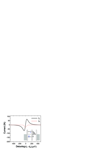
Figure 4: (Color online) QPC-induced charge ($I_{c}=I_{\uparrow}+I_{\downarrow}$) and spin ($I_{s}=I_{\uparrow}-I_{\downarrow}$) currents through a DQD when a static magnetic field is applied at the left dot. Here $\Gamma_{L}=\Gamma_{R}=7.5~{}$MHz and the Zeeman splitting is $\Delta_{z}=20~{}\mu$eV. The other parameters are the same as those in Fig. 3(a). Inset: Schematic diagram of the energy levels in the DQD at $\epsilon_{1}=\epsilon_{2}$.

In Fig. 4, the charge current ($I_{c}=I_{\uparrow}+I_{\downarrow}$) and the spin current ($I_{s}=I_{\uparrow}-I_{\downarrow}$) are plotted versus the energy detuning $\varepsilon_{1}-\varepsilon_{2}$ when $\Gamma_{L}=\Gamma_{R}$. At zero detuning with $\varepsilon_{1}=\varepsilon_{2}$, the charge current is zero and the spin current reaches its maximum. This is because electrons with opposite spins are transported with the same effective rate but in opposite directions. Therefore, a pure spin current without a charge current can be driven by a QPC in this proposed device. A charge current is also induced at non-vanishing detuning ($|\varepsilon|>0$), but its direction is sensitive to the sign of $\varepsilon$. Specifically, the charge current is positive when $\varepsilon_{1}>\varepsilon_{2}$ and negative vice versa. The underlying mechanism can be demonstrated as follows. When the energy detuning is deviated from the zero detuning point, e.g., $\varepsilon_{1}>\varepsilon_{2}$, the absolute value of the spin-up current transporting from the left to the right decreases, while that of the spin-down current transporting from the right to the left increases. This results in a positive charge current tunneling through the DQD. In contrast to other schemes, including electron spin resonance KoppensNature06 or photon-assisted tunneling OosterkampNature98 in QDs, our proposal does not require a fast and strong oscillating magnetic field. Moreover, unlike the partially polarized spin current through a QD driven by a spin bias LuPRB08 or spin-orbit interaction,SunPRL07 a pure spin current without a charge current can be generated here and the amplitude is tunable via the voltage across the QPC.

In quantum transport experiments, the most well-established readout devices are charge detectors. However, these charge-sensitive devices are insensitive to spins. Because of the unique properties of the spin current in our proposed setup, charge detectors can be used to indirectly reveal the existence of the spin current. As shown in Fig. 4, the spin current is symmetric about the energy detuning $\varepsilon_{1}-\varepsilon_{2}$, but the charge current has an asymmetric dependence. If the measured charge current is demonstrated to be asymmetric about $\varepsilon$, as predicted in Fig. 4, it serves as a characteristic feature indicating that a pure spin current occurs at the zero detuning point in our present proposal.

VI Conclusion

In our approach, the current through the zero-bias DQD is due to the backaction of the QPC. This mechanism predicts that the rate for electrons tunneling out of the zero-bias DQD is proportional to the bias voltage applied across the QPC [see Eq. (LABEL:Fout)]. However, in Ref. Gasser09, , where the DQD is assumed to be coupled to acoustic phonons [see Eq. (A4) in Ref. Gasser09, ], this tunneling rate has a polynomial relation with the bias voltage across the QPC. We suggest that, using the setup fabricated in Ref. Gasser09, , one can measure the rate for electrons tunneling out of the DQD as a function of the bias voltage across the QPC to distinguish between these two mechanisms.

In conclusion, we have developed a ME approach to study the backaction of a charge detector (QPC) on a DQD. We show that an electron in the DQD can be excited from its ground state to the excited state when the energy emitted by the QPC exceeds the eigenenergy difference. This agrees well with the observations in two recent experiments.Gustavsson07 ; Gasser09 Moreover, we propose a new scheme to drive a pure spin current by a QPC in the absence of a charge current.

- (1) J. M. Elzerman, R. Hanson, L. H. Willems van Beveren, B. Witkamp, L. M. K. Vandersypen, and L. P. Kouwenhoven, Nature (London) 430, 431 (2004).
- (2) J. R. Petta, A. C. Johnson, C. M. Marcus, M. P. Hanson, and A. C. Gossard, Phys. Rev. Lett. 93, 186802 (2004).
- (3) L. DiCarlo, H. J. Lynch, A. C. Johnson, L. I. Childress, K. Crockett, C. M. Marcus, M. P. Hanson, and A. C. Gossard, Phys. Rev. Lett. 92, 226801 (2004).
- (4) T. Hayashi, T. Fujisawa, H. D. Cheong, Y. H. Jeong, and Y. Hirayama, Phys. Rev. Lett. 91, 226804 (2003).
- (5) M. Field, C. G. Smith, M. Pepper, D. A. Ritchie, J. E. F. Frost, G. A. C. Jones, and D. G. Hasko, Phys. Rev. Lett. 70, 1311 (1993).
- (6) J. M. Elzerman, R. Hanson, J. S. Greidanus, L. H. Willems van Beveren, S. De Franceschi, L. M. K. Vandersypen, S. Tarucha, and L. P. Kouwenhoven, Phys. Rev. B 67, 161308(R) (2003).
- (7) H. S. Goan, G. J. Milburn, H. M. Wiseman, and H. B. Sun, Phys. Rev. B 63, 125326 (2001).
- (8) S. A. Gurvitz, Phys. Rev. B 56, 15215 (1997).
- (9) S. H. Ouyang, C. H. Lam, and J. Q. You, J. Phys.: Condens Matter 18, 115511 (2006).
- (10) S. Gustavsson, M. Studer, R. Leturcq, T. Ihn, K. Ensslin, D. C. Driscoll, and A. C. Gossard, Phys. Rev. Lett. 99, 206804 (2007).
- (11) U. Gasser, S. Gustavsson, B. Küng, K. Ensslin, T. Ihn, D. C. Driscoll, and A. C. Gossard, Phys. Rev. B 79, 035303 (2009).
- (12) R. Aguado and L. P. Kouwenhoven, Phys. Rev. Lett. 84, 1986 (2000).
- (13) E. Onac , F. Balestro, L. H. Willems van Beveren, U. Hartmann, Y.V. Nazarov, and L. P. Kouwenhoven, Phys. Rev. Lett. 96, 176601 (2006); E. Zakka-Bajjani, J. Ségala, F. Portier, P. Roche, and D. C. Glattli, Phys. Rev. Lett. 99, 236803 (2007).
- (14) V. S. Khrapai, S. Ludwig, J. P. Kotthaus, H. P. Tranitz, and W. Wegscheider, Phys. Rev. Lett. 97, 176803 (2006).
- (15) T. M. Stace and S. D. Barrett, Phys. Rev. Lett. 92, 136802 (2004).
- (16) J. Q. You and H. Z. Zheng, Phys. Rev. B 60, 13314 (1999).
- (17) S. H. Ouyang, C. H. Lam, and J. Q. You, arXiv: 0902.3085v1 (unpublised).
- (18) K. Blum, Density Matrix Theory and Applications (Plenum, New York, 1996), Chap. 8.
- (19) N. Lambert, I. Mahboob, M. Pioro-Ladriere, Y. Tokura, S. Tarucha, and H. Yamaguchi, Phys. Rev. Lett. 100, 136802 (2008).
- (20) F. H. L. Koppens, C. Buizert, K. J. Tielrooij, I. T. Vink, K. C. Nowack, T. Meunier, L. P. Kouwenhoven, and L. M. K. Vandersypen, Nature (London) 442, 766 (2006).
- (21) T. H. Oosterkamp, T. Fujisawa, W. G. van der Wiel, K. Ishibashi, R. V. Hijman, S. Tarucha, and L. P. Kouwenhoven, Nature (London) 395, 873 (1998).
- (22) H. Z. Lu and S. Q. Shen, Phys. Rev. B 77, 235309 (2008).
- (23) Q. F. Sun, X. C. Xie, and J. Wang, Phys. Rev. Lett. 98, 196801 (2007).