On link homology theories
from extended cobordisms

Abstract.

This paper is devoted to the study of algebraic structures leading to link homology theories. The originally used structures of Frobenius algebra and/or TQFT are modified in two directions. First, we refine 2–dimensional cobordisms by taking into account their embedding into $\mathbb{R}^{3}$. Secondly, we extend the underlying cobordism category to a 2–category, where the usual relations hold up to 2–isomorphisms. The corresponding abelian 2–functor is called an extended quantum field theory (EQFT). We show that the Khovanov homology, the nested Khovanov homology, extracted by Stroppel and Webster from Seidel–Smith construction, and the odd Khovanov homology fit into this setting. Moreover, we prove that any EQFT based on a ${\mathbb{Z}}_{2}$–extension of the embedded cobordism category which coincides with Khovanov after reducing the coefficients modulo 2, gives rise to a link invariant homology theory isomorphic to those of Khovanov.

Introduction

In his influential paper [7], Khovanov constructed a link homology theory categorifying the Jones polynomial. During few years, this categorification was considered to be essentially unique, since the underlying $(1+1)$ TQFT was known to be determined by its Frobenius system and all rank two Frobenius systems were fully classified [8]. However, in [13] Ozsvath, Rasmussen and Szabo came up with a new categorification of the Jones polynomial, which agrees with Khovanov’s one after reducing the coefficients modulo two. The underlying algebraic structure of the odd Khovanov homology can not be described in terms of the Frobenius algebra.

This fact attracts attention again to the question of description and classification of algebraic structures leading to link homology theories. In this paper, we provide an evidence to the fact that the appropriate algebraic structure is given by an extended quantum field theory (EQFT). A EQFT here is a 2–functor from a certain (semistrict) monoidal 2–category of cobordisms, called an extension, to an abelian category. Given a cobordism category by specifying its generators and relations, the 2–category is constructed by requiring the relations to be satisfied up to 2–isomorphisms. Furthermore, such a 2–category is called an extension of the original cobordism category, if the automorphism group of any 1–morphism is trivial. A simple example of an extension is a ${\mathbb{Z}}_{2}$–extension, where the 2–morphisms are just plus or minus the identity. Notice that extensions can be defined for both strict and semistrict monoidal 2–categories and the resulting EQFT will also be called strict and semistrict respectively.

The usage of the word “extension” in our setting is motivated by the fact that after replacing the original category by a group we will get a usual extension of that group. Those extensions are classified by the second cohomology classes of the group. Therefore, our approach can serve as a definition for the second cohomology of a category. A quite different notion of an extended topological field theory (ETFT) was introduced and studied in [15].

In this paper, we construct extensions of the category of 2–dimensional cobordisms $\operatorname{Cob}$ and of the category of embedded 2–cobordisms modulo the unknotting relation $\operatorname{NesCob}$. In the first case, we recover the Khovanov and the odd Khovanov homologies, as strict (trivial) and semistrict extensions respectively. In the second case, we construct so–called nested Khovanov homology, extracted by Stroppel and Webster [16] from the algebraic counterpart of the Seidel–Smith construction. In addition, we show that the last theory is equivalent to those of Khovanov. More precisely, for a given diagram $D$, let us denote by $\left[\!\!\left[D\right]\!\!\right]$ its Khovanov hypercube of resolutions. Applying the Khovanov TQFT, we get a complex $F_{\operatorname{Kh}}\left[\!\!\left[D\right]\!\!\right]$. On the other hand, using the nested Frobenius system, defined in Section 2.3, we get the complex $F\left[\!\!\left[D\right]\!\!\right]$.

Theorem 1.

Given a diagram $D$ of a link $L$, the complexes $F_{\operatorname{Kh}}\left[\!\!\left[D\right]\!\!\right]$ and $F\left[\!\!\left[D\right]\!\!\right]$ are isomorphic.

Once the equivalence between the geometric construction of Seidel–Smith and the algebraic one of Cautis–Kamnitzer is established rigorously, this theorem can be used to finalize the proof of the Seidel–Smith conjecture.

A similar result was independently proved by a student of C. Stroppel.

The last result of the paper is the classification of all rank two strict ${\mathbb{Z}}_{2}$–extensions of $\operatorname{NesCob}$.

Theorem 2.

Any strict EQFT based on a ${\mathbb{Z}}_{2}$–extension of $\operatorname{NesCob}$, which agrees with Khovanov’s TQFT after reducing the coefficients modulo 2, gives rises to a link invariant homology theory isomorphic to those of Khovanov.

A challenging open problem is to classify all semistrict EQFTs based on $\operatorname{NesCob}$, which associate to a circle a rank two module. More generally, the problem is to compute the second cohomology of $\operatorname{NesCob}$ and construct cocycles restricting to the Schur cocycle of the symmetric group.

An interesting algebraic system underlying the categorification of the Kauffman skein module [1], [18] was proposed recently by Carter and Saito [5]. We wonder whether our approach could be extended to include their setting.

The paper is organized as follows. In the first sections we define the categories $\operatorname{Cob}$, $\operatorname{NesCob}$ and their extensions. Theorems 1 and 2 are proved in Section 3. In the last section, odd Khovanov homology is realized as an extension of $\operatorname{Cob}$.

Acknowledgment

The authors would like to thank Catharina Stroppel, Krzysztof Putyra, Alexander Shumakovitch, Christian Blanchet and Aaron Lauda for interesting discussions and to Dror Bar–Natan for the permission to use his picture of the Khovanov hypercube.

1. The category of 2–cobordisms and its extensions

1.1. The category $\operatorname{Cob}$

Definition 1.1.

The objects of $\operatorname{Cob}$ are finite ordered set of circles. The morphisms are isotopy classes of smooth 2–dimensional cobordisms. The composition is given by gluing of cobordisms.

The category $\operatorname{Cob}$ is a strict symmetric monoidal category with the monoidal product given by the ordered disjoint union and the identity given by the cylinder cobordism. In particular, we obtain a natural embedding of the symmetric group in $n$ letters into the automorphism group of $n$ circles.

By using Morse theory, one can decompose any 2–cobordism into pairs of pants, caps, cups and permutations, proving the following well–known presentation of $\operatorname{Cob}$ (see e.g. [6])

Theorem 1.2.

The morphisms of $\operatorname{Cob}$ are generated by

subject to the following relations:

(1) Commutativity and co-commutativity relation

(2) Associativity and coassociativity relations

(3) Frobenius relations

(4) Unit and Counit relations

(5) Permutation relations

(6) Unit-Permutations and Counit-Permutation relations

(7) Merge-Permutation and Split-Permutation relations

For a commutative unital ring $R$, let $R$-$\operatorname{Mod}$ be the category of finite projective modules over $R$. A (1+1)–dimensional topological quantum field theory (TQFT) is a symmetric (strict) monoidal functor from $\operatorname{Cob}$ to $R$-$\operatorname{Mod}$. Such TQFTs are in $1:1$ correspondence with so–called Frobenius systems (compare [9]).

One important application of Frobenius systems is Khovanov’s categorification of the Jones polynomial [7].

In what follows we will assume that $\operatorname{Cob}$ is a pre–additive category. This means we supply the set of morphisms (between any two given objects) with the structure of an abelian group by allowing formal ${\mathbb{Z}}$–linear combinations of cobordisms and extend the composition maps bilinearly.

1.2. Extensions of categories

In this section we use the language of 2–categories. A 2–category is a category where any set of morphisms has a structure of a category, i.e. we allow morphisms between morphisms called 2–morphisms. Given a 2–category $M$, the 2–morphisms of $M$ can be composed in two ways. For any three objects $a,b,c$ of $M$, the composition in the category ${\operatorname{Mor}}_{M}(a,b)$ is called vertical composition and the bifunctor $*:{\operatorname{Mor}}_{M}(a,b)\times{\operatorname{Mor}}_{M}(b,c)\to{\operatorname{Mor}}_{M}(a,c)$ is called horizontal composition. These compositions are required to be associative and satisfy an interchange law (see [12] for more details).

Semistrict monoidal 2–categories can be considered as a weakening of monoidal 2–categories, where monoidal and interchange rules hold up to natural isomorphisms (compare [10, Proposition 17]).

Assume $\cal C$ is a strict monoidal category, whose set of morphisms is given by generators and relations.

Definition 1.3.

An extension of $\cal C$ is the semistrict monoidal 2–category $\operatorname{Ex\cal C}$, which has the same set of objects as $\cal C$. The 1–morphisms of $\operatorname{Ex\cal C}$ are compositions of generators of $\cal C$. The 2–morphisms are

• the identity automorphism of any 1–morphism of $\cal C$;

• a 2–isomorphism between any two 1–morphisms subject to a relation in ${\mathcal{C}}$.

This imposes a so–called “cocycle” condition on the set of 2–morphisms, since any composition of 2–morphisms going from a given 1–morphism to itself should be equal to the identity or any closed loop of 2–morphisms is trivial.

An example of an extension is given by a weak monoidal category $(M,\otimes,1,\alpha,\lambda,\rho)$ where $\alpha$, $\lambda$ and $\rho$ are considered as 2–isomorphisms and the cocycle condition holds due to MacLane’s coherence theorem [12, Chapter VII]. In the case, when $\cal C$ is $\operatorname{Cob}$ restricted to connected cobordisms, (i.e. permutation is removed from the set of generators in Theorem 1.2 as well as relations (1),(5), (6) and (7)), then any pseudo Frobenius algebra, described in [10, Proposition 25], defines an extension $\operatorname{Ex\cal C}$. The cocycle condition holds due to Lemmas 32, 33 in [10].

Providing $\cal C$ with a structure of a pre–additive category, we have a natural ${\mathbb{Z}}$–action on the set of 1–morphisms, restricting to ${\mathbb{Z}}_{2}=\{1,-1\}$, the group of two elements written multiplicatively, we can define a ${\mathbb{Z}}_{2}$–extension of $\cal C$, in which the 2–morphisms are just plus or minus the identity. Note that in this case $\operatorname{Ex\cal C}$ can be considered as a weak monoidal category, with the same set of generating 1–morphisms as $\cal C$, but with sign modified relations.

For any cobordism category $\cal C$, an extended quantum field theory (EQFT) based on $\cal C$ is a bifunctor from $\operatorname{Ex\cal C}$ to $R$-$\operatorname{Mod}$, mapping 2–morphisms to natural transformations of $R$–modules. The EQFT is called strict if $\operatorname{Ex\cal C}$ is strict.

2. Embedded cobordisms

Let $S^{\amalg a}$ be the disjoint union of $a$ copies of a circle smoothly embedded into a plane. Note that the embedding induces a partial order on the set of circles as follows. For two circles $c_{1}$ and $c_{2}$, we say $c_{1}<c_{2}$, if $c_{1}$ is inside $c_{2}$.

Definition 2.1.

The objects of $\operatorname{NesCob}$ are finite collections of circles embedded into a plane. The morphisms are generated by

subject to the following sets of relations:

(1) Frobenius type relations

(2) Associativity type relations

(3) Coassociativity type relations

(4) Cancellation

(5) Torus relation

In addition, the merge, the split, the birth, the death and the permutation are still subject to all the relations of Theorem 1.2.

Remark 2.1.

The relations of Definition 2.1 can also be described as follows:

\begin{picture}(19171.0,3914.0)(7478.0,-7976.0)\end{picture}\begin{picture}(32622.0,5072.0)(2802.0,-9197.0)\end{picture}\begin{picture}(19687.0,7853.0)(3245.0,-12160.0)\end{picture}\begin{picture}(2012.0,2458.0)(3838.0,-11269.0)\end{picture}

where the black circle corresponds to the starting configuration of circles, and the dashed arcs correspond to the operations which are performed. Notice that changing the order of operations produce the two different sides of the relations in Definition 2.1. In addition, associativity of the merge, the coassociativity of the split and the usual Frobenius relation are also depicted here.

The category $\operatorname{NesCob}$ is a symmetric strict monoidal category with a tensor product given by a partially ordered disjoint union, i.e. circles on the same level of nestedness are ordered. In particular, we obtain a natural embedding of the symmetric group into the automorphisms of any object, permuting circles not ordered by nestedness and at the same level of nestedness.

Any morphism in $\operatorname{NesCob}$ is the composite of such a permutation and the tensor product of connected morphisms of $\operatorname{NesCob}$.

Lemma 2.2.

Any connected morphism in $\operatorname{NesCob}$ has the following normal form:

\begin{picture}(24325.0,9369.0)(6704.0,-18032.0)\end{picture}

Proof.

Assume that the boundary of our connected genus $g$ cobordism $C$ consists of $a$ incoming circles and $b$ outgoing ones. Let us suppose that $C$ is a composition of $B$ births, $D$ deaths, $M$ merges and $S$ splits. Then we have

$$2-2g-a-b=B+D-M-S,\quad\quad a-M+B=b-S+D$$

or

$$M=a+g-1+B,\quad\quad S=b+g-1+D$$

We arrive at the normal form if we will be able to push all merges (resp. splits) to the incoming (resp. outgoing) boundary of $C$. From the above formulas we see that $B$ merges and $D$ splits will cancel with the births and deaths, respectively, and $g$ splits and merges put together will create $g$ handles. The remaining $a-1$ merges commute with any split (nested or not nested one) due to the Frobenius type relations. Finally using the associativity type relations, we can commute nested and unnested merges (resp. splits) and arrive at the form in Figure 1.

\begin{picture}(38350.0,9369.0)(-7321.0,-18032.0)\end{picture}

Figure 1. Normal form with inner and outer handles

Furthermore applying the Torus relation, one can now reduce to the normal form. ∎

2.1. Embedded cobordisms

Definition 2.3.

A smoothly embedded 2–dimensional cobordism from $S^{\amalg a}$ to $S^{\amalg b}$ is a pair $(F,\phi)$, where $F$ a smooth 2–dimensional surface whose boundary consists of $a+b$ circles and $\phi:F\hookrightarrow\mathbb{R}^{2}\times[0,1]$ is a smooth embedding, such that $\phi|_{\partial F}\cap\mathbb{R}^{2}\times\{0\}=S^{\amalg a}$ and $\phi|_{\partial F}\cap\mathbb{R}^{2}\times\{1\}=S^{\amalg b}$.

Definition 2.4.

The objects of $\operatorname{EmbCob}$ are circles smoothly embedded into a plane. The morphisms are isotopy classes of smoothly embedded 2–dimensional cobordisms subject to the unknotting relation:

The composition is given by gluing along the boundary.

The category $\operatorname{EmbCob}$ is again a symmetric strict monoidal category with a tensor product given by the partially ordered disjoint union and with the action of the permutation group depending on nestedness.

Theorem 2.5.

The category $\operatorname{EmbCob}$ is isomorphic to the category $\operatorname{NesCob}$.

Proof.

By [6], any smooth 2–cobordism allows a pair of pants decomposition. Modulo the unknotting relation, there are two ways to embed a pair of pants into $\mathbb{R}^{3}$, providing the list of generators in Definition 2.1. The relations do not change the isotopy class of an embedded cobordism and allow to bring it into a normal form. It remains just to say, that the normal forms of two equivalent connected cobordisms coincide. ∎

2.2. Strict ${\mathbb{Z}}_{2}$–extension

Assume $\operatorname{NesCob}$ is a pre–additive category.

Definition 2.6.

Let $\operatorname{NesCob}_{1}$ be the strict monoidal 2–category obtained from $\operatorname{NesCob}$ by replacing the torus relation with

(T1)

Lemma 2.7.

$\operatorname{NesCob}_{1}$ is a ${\mathbb{Z}}_{2}$–extension of $\operatorname{NesCob}$.

Proof.

The only non–trivial 2–morphism corresponds to the torus relation. It remains to show that the automorphism group of any 1–morphism is trivial. By Bergman’s Diamond Lemma [4], it suffices to check that any cube with T1 face has an even number of anticommutative faces. This is a simple case by case check. The 10 cubes to check are depicted in Figure 2.

\begin{picture}(20787.0,7435.0)(3688.0,-16246.0)\end{picture}

Figure 2. Cocycle conditions for $\operatorname{NesCob}_{1}$

∎

Remark 2.2.

Notice that any element of $\operatorname{NesCob}_{1}$ does still have a normal form, which corresponds to the usual one plus the information of the parity of the number of inner 1–handles in Figure 1.

2.3. Nested Frobenius system

In this section we construct a strict EQFT based on $\operatorname{NesCob}_{1}$, as proposed by Stroppel [17].

As in [7], let us consider the 2–dimensional module $A:={\mathbb{Z}}[t]\langle{\rm\begin{picture}(0.75,1.0)\put(0.0,0.0){$1$}\put(0.34,0.0){\line(0,1){0.65}} \end{picture}},X\rangle$ over the polynomial ring $R:={\mathbb{Z}}[t]$ in one variable. We denote by the image of 1 under the embedding $\eta:R\to A$. For $\varepsilon\in\{0,1\}$, we define two kinds of a multiplication $m_{\varepsilon}:A\otimes A\to A$ as follows:

(1) $$m_{\varepsilon}:\left\{\begin{array}[]{l@{\quad\mapsto\quad}r}{\rm\begin{picture}(0.75,1.0)\put(0.0,0.0){$1$}\put(0.34,0.0){\line(0,1){0.65}} \end{picture}}\otimes{\rm\begin{picture}(0.75,1.0)\put(0.0,0.0){$1$}\put(0.34,0.0){\line(0,1){0.65}} \end{picture}}&{\rm\begin{picture}(0.75,1.0)\put(0.0,0.0){$1$}\put(0.34,0.0){\line(0,1){0.65}} \end{picture}}\\ {\rm\begin{picture}(0.75,1.0)\put(0.0,0.0){$1$}\put(0.34,0.0){\line(0,1){0.65}} \end{picture}}\otimes X&X\\ X\otimes{\rm\begin{picture}(0.75,1.0)\put(0.0,0.0){$1$}\put(0.34,0.0){\line(0,1){0.65}} \end{picture}}&(-1)^{\varepsilon}X\\ X\otimes X&(-1)^{\varepsilon}t\end{array}\right.$$

Further, we define two comultiplications $\Delta_{\varepsilon}:A\to A\otimes A$ and a counit $\epsilon:A\to R$ as follows.

(2) $$\Delta_{\varepsilon}:\left\{\begin{array}[]{l@{\quad\mapsto\quad}r}{\rm\begin{picture}(0.75,1.0)\put(0.0,0.0){$1$}\put(0.34,0.0){\line(0,1){0.65}} \end{picture}}&X\otimes{\rm\begin{picture}(0.75,1.0)\put(0.0,0.0){$1$}\put(0.34,0.0){\line(0,1){0.65}} \end{picture}}+(-1)^{\varepsilon}\;{\rm\begin{picture}(0.75,1.0)\put(0.0,0.0){$1$}\put(0.34,0.0){\line(0,1){0.65}} \end{picture}}\otimes X\\ X&X\otimes X+(-1)^{\varepsilon}\;t{\rm\begin{picture}(0.75,1.0)\put(0.0,0.0){$1$}\put(0.34,0.0){\line(0,1){0.65}} \end{picture}}\otimes{\rm\begin{picture}(0.75,1.0)\put(0.0,0.0){$1$}\put(0.34,0.0){\line(0,1){0.65}} \end{picture}}\\ \end{array}\right.\quad\quad\epsilon:\left\{\begin{array}[]{l@{\quad\mapsto\quad}r}{\rm\begin{picture}(0.75,1.0)\put(0.0,0.0){$1$}\put(0.34,0.0){\line(0,1){0.65}} \end{picture}}&0\\ X&1\\ \end{array}\right.$$

The functor $F:\operatorname{NesCob}_{1}\to R$-$\operatorname{Mod}$ maps any object $S^{\amalg a}$ to $A^{\otimes a}$ and is defined on the generating morphisms as follows:

(3) $$F\left(\begin{array}[]{c}\end{array}\right)=m_{0},\quad F\left(\begin{array}[]{c}\end{array}\right)=\Delta_{0},$$

(4) $$F\left(\begin{array}[]{c}\end{array}\right)=m_{1},\quad F\left(\begin{array}[]{c}\end{array}\right)=\Delta_{1},$$

(5) $$F\left(\begin{array}[]{c}\end{array}\right)=\eta,\quad F\left(\begin{array}[]{c}\end{array}\right)=\epsilon,$$

The convention is that in $A\otimes A$ the first factor corresponds to the inner circle. It is easy to see that $F$ preserves all the relations listed in Definition 2.1.

Let us introduce a grading on $A$ by putting

$$\operatorname{deg}(t):=-4,\quad\operatorname{deg}(X):=-1,\quad\operatorname{deg}({\rm\begin{picture}(0.75,1.0)\put(0.0,0.0){$1$}\put(0.34,0.0){\line(0,1){0.65}} \end{picture}}):=1$$

On the tensor product $A^{\otimes n}$ the grading is given by $\operatorname{deg}(a_{1}\otimes\dots\otimes a_{n}):=\operatorname{deg}(a_{1})+\dots+\operatorname{deg}(a_{n})$.

There exist a natural grading on $\operatorname{NesCob}$ given by the Euler characteristic of cobordisms. As in Khovanov’s case if $t=0$, $F$ is grading preserving.

3. Nested Khovanov homology

3.1. Khovanov’s hypercube

Suppose we have a generic diagram $D$ of an oriented link $L$ in $S^{3}$ with $c$ crossings. By resolving crossings of $D$ in two ways as prescribed by the Kauffman skein relations, one can associate to $D$ a $c$–dimensional cube of resolutions (compare [7] or [2]). The vertices of the cube correspond to the configurations of circles obtained after smoothing of all crossings in $D$. For any crossing, two different smoothings are allowed: the $0$– and the $1$–smoothings. Therefore, we have $2^{c}$ vertices. After numbering the crossings of $D$, we can label the vertices of the cube by $c$–letter strings of $0$’s and $1$’s, specifying the smoothing chosen at each crossing. The cube is skewered along its main diagonal, from $00...0$ to $11...1$. The number of 1 in the labeling of a vertex is equal to its ‘height’ $k$. The cube is displayed in such a way that the vertices of height $k$ project down to the point $r:=k-c_{-}$, where $c_{\pm}$ are the numbers of positive, resp. negative crossings in $D$ (see Figure 3).

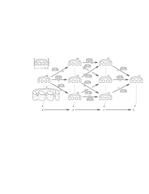
Figure 3. The cube of resolutions for the trefoil

Two vertices of the hypercube are connected by an edge if their labellings differ by one letter. In Figure 3, this letter is labeled by $*$. The edges are directed (from the vertex where this letter is $0$ to the vertex where it is $1$). The edges correspond to a saddle cobordisms from the tail configuration of circles to the head configuration (compare Figure 3).

We denote this hypercube of resolutions by $\left[\!\!\left[D\right]\!\!\right]$, and would like to interpret it as a complex. The $r$th chain “space” $\left[\!\!\left[D\right]\!\!\right]^{r}$ is a formal direct sum of the $\frac{c!}{k!(c-k)!}$ “spaces” at height $k$ in the hypercube and the sum of “maps” with tails at height $k$ defines the $r$th differential. To achieve $\partial^{2}=0$, we assign a minus to any edge which has an odd number of 1’s before $*$ in its labeling.

Applying (1+1) TQFT $F_{Kh}$ to $\left[\!\!\left[D\right]\!\!\right]$, which sends any merge to $m_{0}$ and any split to $\Delta_{0}$, we get a complex of $R$-modules $(F_{\operatorname{Kh}}\left[\!\!\left[D\right]\!\!\right],\partial_{\operatorname{Kh}})$. Its graded homology groups, known as Khovanov homology, are link invariants and the graded Euler characteristic is given by the Jones polynomial.

3.2. Nested homology

Applying $F$ to the Khovanov hypercube, one can define a chain complex as follows. The $r$th chain group will be $F\left[\!\!\left[D\right]\!\!\right]^{r}$, the image of $\left[\!\!\left[D\right]\!\!\right]^{r}$ after applying the functor $F$, and the maps are defined by applying $F$ to the corresponding cobordisms. The main difference to the Khovanov case is that here not all faces are commutative. More precisely, the square corresponding to the Torus relation $(T1)$ is anti–commutative. However, by the definition of the ${\mathbb{Z}}_{2}$–extension, the 2–cochain $\psi\in H^{2}(B,\mathbb{Z}/2\mathbb{Z})$ ($B$ is the hypercube) which associates $1$ to any anticommutative face of the hypercube and $-1$ to any commutative one is a cocycle, i.e. it vanishes on the boundary of any cube. Since the cube is contractible, any cocycle is a coboundary. Consequently, there exists a function $\epsilon:{\cal E}\to{\mathbb{Z}}_{2}$ from the set of edges of the hypercube to ${\mathbb{Z}}_{2}$, called a sign assignment, such that $\epsilon(e_{1})\epsilon(e_{2})\epsilon(e_{3})\epsilon(e_{4})=\psi(D)$ for any four edges $e_{1},\dots,e_{4}$ forming a square $D$. Hence, multiplying edges of the hypercube by the signs $\epsilon$, we get a chain complex $(F\left[\!\!\left[D\right]\!\!\right],\partial_{\epsilon})$. It is easy to see that this complex is independent on the choice of a sign assignment.

Lemma 3.1.

Given two sign assignments $\epsilon$ and $\epsilon^{\prime}$, the chain complexes $(F\left[\!\!\left[D\right]\!\!\right],\partial_{\epsilon})$ $(F\left[\!\!\left[D\right]\!\!\right],\partial_{\epsilon^{\prime}})$ are isomorphic.

Proof.

The product $\epsilon\epsilon^{\prime}$ is a 1–cocycle. Since the hypercube is contractible, this 1-cocycle is a coboundary of a 0–cochain $\eta:{\cal V}\to{\mathbb{Z}}_{2}$. The identity map times $\eta$ provides the required isomorphism. ∎

In the case, when $t=0$, the homology groups of $(F\left[\!\!\left[D\right]\!\!\right],\partial)$ are graded and the graded Euler characteristic coincides with the Jones polynomial. If $t\neq 0$, then $\operatorname{deg}$ defines a filtration on our chain complex, similar to the one considered by Lee [11].

Our next aim is to show that the complex we just constructed is isomorphic to the Khovanov complex.

3.3. Proof of Theorem 1

We have to show that $(F\left[\!\!\left[D\right]\!\!\right],\partial)$ and $(F_{\operatorname{Kh}}\left[\!\!\left[D\right]\!\!\right],\partial_{\operatorname{Kh}})$ are isomorphic.

For any circle $c$ in $S^{\amalg k}$, we define $\operatorname{nes}(c)$ to be the number of circles in $S^{\amalg k}$ containing $c$ inside. Further, we define an endomorphism $\phi_{k}$ of $F(S^{\amalg k})$ as follows: For a copy of $A$ associated with $c$, we put

(6) $$\phi_{c}:\left\{\begin{array}[]{l@{\quad\mapsto\quad}r}{\rm\begin{picture}(0.75,1.0)\put(0.0,0.0){$1$}\put(0.34,0.0){\line(0,1){0.65}} \end{picture}}&{\rm\begin{picture}(0.75,1.0)\put(0.0,0.0){$1$}\put(0.34,0.0){\line(0,1){0.65}} \end{picture}}\\ X&(-1)^{\operatorname{nes}(c)}\;X\\ \end{array}\right.$$

Then $\phi_{k}$ is the composition of $\phi_{c}$ for all circles in $S^{\amalg k}$. By abuse of notation $\phi_{k}$ depends not only on $k$ but also on the configuration of circles in $S^{\amalg k}$.

Given a link diagram $D$ with $d$ crossings, consider two Khovanov’s hypercubes of resolutions associated with $D$. Apply $F$ to one of them and $F_{\operatorname{Kh}}$ to the other and do not use any sign assignment, i.e. all squares in $F_{\operatorname{Kh}}\left[\!\!\left[D\right]\!\!\right]$ are commutative. Further, observe that with each vertex of the hypercube, there is a copy of $A^{\otimes k}$, for a certain $k$, associated. Applying $\phi_{k}$ to any such vertex, we get a map $\Phi$ with the source $(F\left[\!\!\left[D\right]\!\!\right],\partial)$ and the target $(F_{\operatorname{Kh}}\left[\!\!\left[D\right]\!\!\right],\partial_{\operatorname{Kh}})$, without any sign assignments. Our next goal is to see that there exists a sign assignment on the $(d+1)$–dimensional hypercube $\left[\!\!\left[D\right]\!\!\right]\times[0,1]$ making $\Phi$ to a chain map.

For this, it is enough to check that each $3$–dimensional cube in this $(d+1)$–dimensional hypercube contains an even number of anticommutative faces. Note that there are three different cases: (1) the cube is contained in the source hypercube, (2) the cube is contained in the target hypercube, (3) the cube contains exactly one face in the source hypercube and one face in the target hypercube. The first case follows from Lemma 2.7 and the second from the fact that $F_{\operatorname{Kh}}$ is a $(1+1)$ TQFT. The third case rely on a case by case check. Note that all faces in the source hypercube correspond to relations in $\operatorname{NesCob}_{1}$. Hence, we have to check the claim for any cube, whose upper face is a relation in $\operatorname{NesCob}_{1}$, the lower face is the corresponding Khovanov square and whose vertical edges are labeled by $\Phi$. In addition, since the map $\phi_{c}$ depends on $\operatorname{nes}(c)$ explicitly, we have to ensure that the claim holds after changing the nestedness of each circle by one. The tables below show that any cube of type (3) does have only commutative or anticommutative faces. It is left to the reader to check that all cubes of type (3) do have an even number of anticommutative faces. For this one has to consider all cubes where the upper face corresponds to one of the relations in Definition 2.1. Moreover, each cube should be checked twice for different nestedness modulo 2.

	$m_{1}$	$\phi\circ m_{1}$	$\phi$	$m_{0}\circ\phi$
${\rm\begin{picture}(0.75,1.0)\put(0.0,0.0){$1$}\put(0.34,0.0){\line(0,1){0.65}} \end{picture}}\otimes{\rm\begin{picture}(0.75,1.0)\put(0.0,0.0){$1$}\put(0.34,0.0){\line(0,1){0.65}} \end{picture}}$			${\rm\begin{picture}(0.75,1.0)\put(0.0,0.0){$1$}\put(0.34,0.0){\line(0,1){0.65}} \end{picture}}\otimes{\rm\begin{picture}(0.75,1.0)\put(0.0,0.0){$1$}\put(0.34,0.0){\line(0,1){0.65}} \end{picture}}$
${\rm\begin{picture}(0.75,1.0)\put(0.0,0.0){$1$}\put(0.34,0.0){\line(0,1){0.65}} \end{picture}}\otimes X$	$X$	$X$	${\rm\begin{picture}(0.75,1.0)\put(0.0,0.0){$1$}\put(0.34,0.0){\line(0,1){0.65}} \end{picture}}\otimes X$	$X$
$X\otimes{\rm\begin{picture}(0.75,1.0)\put(0.0,0.0){$1$}\put(0.34,0.0){\line(0,1){0.65}} \end{picture}}$	$-X$	$-X$	$-X\otimes{\rm\begin{picture}(0.75,1.0)\put(0.0,0.0){$1$}\put(0.34,0.0){\line(0,1){0.65}} \end{picture}}$	$-X$
$X\otimes X$	$-t$	$-t$	$-X\otimes X$	$-t$

	$m_{1}$	$\phi\circ m_{1}$	$\phi$	$m_{0}\circ\phi$
${\rm\begin{picture}(0.75,1.0)\put(0.0,0.0){$1$}\put(0.34,0.0){\line(0,1){0.65}} \end{picture}}\otimes{\rm\begin{picture}(0.75,1.0)\put(0.0,0.0){$1$}\put(0.34,0.0){\line(0,1){0.65}} \end{picture}}$			${\rm\begin{picture}(0.75,1.0)\put(0.0,0.0){$1$}\put(0.34,0.0){\line(0,1){0.65}} \end{picture}}\otimes{\rm\begin{picture}(0.75,1.0)\put(0.0,0.0){$1$}\put(0.34,0.0){\line(0,1){0.65}} \end{picture}}$
${\rm\begin{picture}(0.75,1.0)\put(0.0,0.0){$1$}\put(0.34,0.0){\line(0,1){0.65}} \end{picture}}\otimes X$	$X$	$-X$	$-{\rm\begin{picture}(0.75,1.0)\put(0.0,0.0){$1$}\put(0.34,0.0){\line(0,1){0.65}} \end{picture}}\otimes X$	$-X$
$X\otimes{\rm\begin{picture}(0.75,1.0)\put(0.0,0.0){$1$}\put(0.34,0.0){\line(0,1){0.65}} \end{picture}}$	$-X$	$X$	$X\otimes{\rm\begin{picture}(0.75,1.0)\put(0.0,0.0){$1$}\put(0.34,0.0){\line(0,1){0.65}} \end{picture}}$	$X$
$X\otimes X$	$-t$	$-t$	$-X\otimes X$	$-t$

	$\Delta_{1}$	$\phi\circ\Delta_{1}$	$\phi$	$\Delta_{0}\circ\phi$
	$X\otimes{\rm\begin{picture}(0.75,1.0)\put(0.0,0.0){$1$}\put(0.34,0.0){\line(0,1){0.65}} \end{picture}}-{\rm\begin{picture}(0.75,1.0)\put(0.0,0.0){$1$}\put(0.34,0.0){\line(0,1){0.65}} \end{picture}}\otimes X$	$-X\otimes{\rm\begin{picture}(0.75,1.0)\put(0.0,0.0){$1$}\put(0.34,0.0){\line(0,1){0.65}} \end{picture}}-{\rm\begin{picture}(0.75,1.0)\put(0.0,0.0){$1$}\put(0.34,0.0){\line(0,1){0.65}} \end{picture}}\otimes X$		$X\otimes{\rm\begin{picture}(0.75,1.0)\put(0.0,0.0){$1$}\put(0.34,0.0){\line(0,1){0.65}} \end{picture}}+{\rm\begin{picture}(0.75,1.0)\put(0.0,0.0){$1$}\put(0.34,0.0){\line(0,1){0.65}} \end{picture}}\otimes X$
$X$	$X\otimes X-t{\rm\begin{picture}(0.75,1.0)\put(0.0,0.0){$1$}\put(0.34,0.0){\line(0,1){0.65}} \end{picture}}\otimes{\rm\begin{picture}(0.75,1.0)\put(0.0,0.0){$1$}\put(0.34,0.0){\line(0,1){0.65}} \end{picture}}$	$-X\otimes X-t{\rm\begin{picture}(0.75,1.0)\put(0.0,0.0){$1$}\put(0.34,0.0){\line(0,1){0.65}} \end{picture}}\otimes{\rm\begin{picture}(0.75,1.0)\put(0.0,0.0){$1$}\put(0.34,0.0){\line(0,1){0.65}} \end{picture}}$	$X$	$X\otimes X+t{\rm\begin{picture}(0.75,1.0)\put(0.0,0.0){$1$}\put(0.34,0.0){\line(0,1){0.65}} \end{picture}}\otimes{\rm\begin{picture}(0.75,1.0)\put(0.0,0.0){$1$}\put(0.34,0.0){\line(0,1){0.65}} \end{picture}}$

	$\Delta_{1}$	$\phi\circ\Delta_{1}$	$\phi$	$\Delta_{0}\circ\phi$
	$X\otimes{\rm\begin{picture}(0.75,1.0)\put(0.0,0.0){$1$}\put(0.34,0.0){\line(0,1){0.65}} \end{picture}}-{\rm\begin{picture}(0.75,1.0)\put(0.0,0.0){$1$}\put(0.34,0.0){\line(0,1){0.65}} \end{picture}}\otimes X$	$X\otimes{\rm\begin{picture}(0.75,1.0)\put(0.0,0.0){$1$}\put(0.34,0.0){\line(0,1){0.65}} \end{picture}}+{\rm\begin{picture}(0.75,1.0)\put(0.0,0.0){$1$}\put(0.34,0.0){\line(0,1){0.65}} \end{picture}}\otimes X$		$X\otimes{\rm\begin{picture}(0.75,1.0)\put(0.0,0.0){$1$}\put(0.34,0.0){\line(0,1){0.65}} \end{picture}}+{\rm\begin{picture}(0.75,1.0)\put(0.0,0.0){$1$}\put(0.34,0.0){\line(0,1){0.65}} \end{picture}}\otimes X$
$X$	$X\otimes X-t{\rm\begin{picture}(0.75,1.0)\put(0.0,0.0){$1$}\put(0.34,0.0){\line(0,1){0.65}} \end{picture}}\otimes{\rm\begin{picture}(0.75,1.0)\put(0.0,0.0){$1$}\put(0.34,0.0){\line(0,1){0.65}} \end{picture}}$	$-X\otimes X-t{\rm\begin{picture}(0.75,1.0)\put(0.0,0.0){$1$}\put(0.34,0.0){\line(0,1){0.65}} \end{picture}}\otimes{\rm\begin{picture}(0.75,1.0)\put(0.0,0.0){$1$}\put(0.34,0.0){\line(0,1){0.65}} \end{picture}}$	$-X$	$-X\otimes X-t{\rm\begin{picture}(0.75,1.0)\put(0.0,0.0){$1$}\put(0.34,0.0){\line(0,1){0.65}} \end{picture}}\otimes{\rm\begin{picture}(0.75,1.0)\put(0.0,0.0){$1$}\put(0.34,0.0){\line(0,1){0.65}} \end{picture}}$

	$m_{0}$	$\phi\circ m_{0}$	$\phi$	$m_{0}\circ\phi$
${\rm\begin{picture}(0.75,1.0)\put(0.0,0.0){$1$}\put(0.34,0.0){\line(0,1){0.65}} \end{picture}}\otimes{\rm\begin{picture}(0.75,1.0)\put(0.0,0.0){$1$}\put(0.34,0.0){\line(0,1){0.65}} \end{picture}}$			${\rm\begin{picture}(0.75,1.0)\put(0.0,0.0){$1$}\put(0.34,0.0){\line(0,1){0.65}} \end{picture}}\otimes{\rm\begin{picture}(0.75,1.0)\put(0.0,0.0){$1$}\put(0.34,0.0){\line(0,1){0.65}} \end{picture}}$
${\rm\begin{picture}(0.75,1.0)\put(0.0,0.0){$1$}\put(0.34,0.0){\line(0,1){0.65}} \end{picture}}\otimes X$	$X$	$X$	${\rm\begin{picture}(0.75,1.0)\put(0.0,0.0){$1$}\put(0.34,0.0){\line(0,1){0.65}} \end{picture}}\otimes X$	$X$
$X\otimes{\rm\begin{picture}(0.75,1.0)\put(0.0,0.0){$1$}\put(0.34,0.0){\line(0,1){0.65}} \end{picture}}$	$X$	$X$	$X\otimes{\rm\begin{picture}(0.75,1.0)\put(0.0,0.0){$1$}\put(0.34,0.0){\line(0,1){0.65}} \end{picture}}$	$X$
$X\otimes X$	$t$	$t$	$X\otimes X$	$t$

	$m_{0}$	$\phi\circ m_{0}$	$\phi$	$m_{0}\circ\phi$
${\rm\begin{picture}(0.75,1.0)\put(0.0,0.0){$1$}\put(0.34,0.0){\line(0,1){0.65}} \end{picture}}\otimes{\rm\begin{picture}(0.75,1.0)\put(0.0,0.0){$1$}\put(0.34,0.0){\line(0,1){0.65}} \end{picture}}$			${\rm\begin{picture}(0.75,1.0)\put(0.0,0.0){$1$}\put(0.34,0.0){\line(0,1){0.65}} \end{picture}}\otimes{\rm\begin{picture}(0.75,1.0)\put(0.0,0.0){$1$}\put(0.34,0.0){\line(0,1){0.65}} \end{picture}}$
${\rm\begin{picture}(0.75,1.0)\put(0.0,0.0){$1$}\put(0.34,0.0){\line(0,1){0.65}} \end{picture}}\otimes X$	$X$	$-X$	$-{\rm\begin{picture}(0.75,1.0)\put(0.0,0.0){$1$}\put(0.34,0.0){\line(0,1){0.65}} \end{picture}}\otimes X$	$-X$
$X\otimes{\rm\begin{picture}(0.75,1.0)\put(0.0,0.0){$1$}\put(0.34,0.0){\line(0,1){0.65}} \end{picture}}$	$X$	$-X$	$-X\otimes{\rm\begin{picture}(0.75,1.0)\put(0.0,0.0){$1$}\put(0.34,0.0){\line(0,1){0.65}} \end{picture}}$	$-X$
$X\otimes X$	$+t$	$+t$	$+X\otimes X$	$+t$

	$\Delta_{0}$	$\phi\circ\Delta_{0}$	$\phi$	$\Delta_{0}\circ\phi$
	$X\otimes{\rm\begin{picture}(0.75,1.0)\put(0.0,0.0){$1$}\put(0.34,0.0){\line(0,1){0.65}} \end{picture}}+{\rm\begin{picture}(0.75,1.0)\put(0.0,0.0){$1$}\put(0.34,0.0){\line(0,1){0.65}} \end{picture}}\otimes X$	$X\otimes{\rm\begin{picture}(0.75,1.0)\put(0.0,0.0){$1$}\put(0.34,0.0){\line(0,1){0.65}} \end{picture}}+{\rm\begin{picture}(0.75,1.0)\put(0.0,0.0){$1$}\put(0.34,0.0){\line(0,1){0.65}} \end{picture}}\otimes X$		$X\otimes{\rm\begin{picture}(0.75,1.0)\put(0.0,0.0){$1$}\put(0.34,0.0){\line(0,1){0.65}} \end{picture}}+{\rm\begin{picture}(0.75,1.0)\put(0.0,0.0){$1$}\put(0.34,0.0){\line(0,1){0.65}} \end{picture}}\otimes X$
$X$	$X\otimes X+t{\rm\begin{picture}(0.75,1.0)\put(0.0,0.0){$1$}\put(0.34,0.0){\line(0,1){0.65}} \end{picture}}\otimes{\rm\begin{picture}(0.75,1.0)\put(0.0,0.0){$1$}\put(0.34,0.0){\line(0,1){0.65}} \end{picture}}$	$X\otimes X+t{\rm\begin{picture}(0.75,1.0)\put(0.0,0.0){$1$}\put(0.34,0.0){\line(0,1){0.65}} \end{picture}}\otimes{\rm\begin{picture}(0.75,1.0)\put(0.0,0.0){$1$}\put(0.34,0.0){\line(0,1){0.65}} \end{picture}}$	$X$	$X\otimes X+t{\rm\begin{picture}(0.75,1.0)\put(0.0,0.0){$1$}\put(0.34,0.0){\line(0,1){0.65}} \end{picture}}\otimes{\rm\begin{picture}(0.75,1.0)\put(0.0,0.0){$1$}\put(0.34,0.0){\line(0,1){0.65}} \end{picture}}$

	$\Delta_{0}$	$\phi\circ\Delta_{0}$	$\phi$	$\Delta_{0}\circ\phi$
	$X\otimes{\rm\begin{picture}(0.75,1.0)\put(0.0,0.0){$1$}\put(0.34,0.0){\line(0,1){0.65}} \end{picture}}+{\rm\begin{picture}(0.75,1.0)\put(0.0,0.0){$1$}\put(0.34,0.0){\line(0,1){0.65}} \end{picture}}\otimes X$	$-X\otimes{\rm\begin{picture}(0.75,1.0)\put(0.0,0.0){$1$}\put(0.34,0.0){\line(0,1){0.65}} \end{picture}}-{\rm\begin{picture}(0.75,1.0)\put(0.0,0.0){$1$}\put(0.34,0.0){\line(0,1){0.65}} \end{picture}}\otimes X$		$X\otimes{\rm\begin{picture}(0.75,1.0)\put(0.0,0.0){$1$}\put(0.34,0.0){\line(0,1){0.65}} \end{picture}}+{\rm\begin{picture}(0.75,1.0)\put(0.0,0.0){$1$}\put(0.34,0.0){\line(0,1){0.65}} \end{picture}}\otimes X$
$X$	$X\otimes X+t{\rm\begin{picture}(0.75,1.0)\put(0.0,0.0){$1$}\put(0.34,0.0){\line(0,1){0.65}} \end{picture}}\otimes{\rm\begin{picture}(0.75,1.0)\put(0.0,0.0){$1$}\put(0.34,0.0){\line(0,1){0.65}} \end{picture}}$	$X\otimes X+t{\rm\begin{picture}(0.75,1.0)\put(0.0,0.0){$1$}\put(0.34,0.0){\line(0,1){0.65}} \end{picture}}\otimes{\rm\begin{picture}(0.75,1.0)\put(0.0,0.0){$1$}\put(0.34,0.0){\line(0,1){0.65}} \end{picture}}$	$-X$	$-X\otimes X-t{\rm\begin{picture}(0.75,1.0)\put(0.0,0.0){$1$}\put(0.34,0.0){\line(0,1){0.65}} \end{picture}}\otimes{\rm\begin{picture}(0.75,1.0)\put(0.0,0.0){$1$}\put(0.34,0.0){\line(0,1){0.65}} \end{picture}}$

To finish, observe that the map $\phi$ composed with a sign assignment is clearly invertible, and hence, is the desired isomorphism. ∎

3.4. Proof of Theorem 2

Let us search for further strict ${\mathbb{Z}}_{2}$–extensions of $\operatorname{NesCob}$ systematically. For $e_{i}\in{\mathbb{Z}}_{2}$ with $i=1,...,10$, we put

(7) $$m_{0}:\left\{\begin{array}[]{l@{\quad\mapsto\quad}r}{\rm\begin{picture}(0.75,1.0)\put(0.0,0.0){$1$}\put(0.34,0.0){\line(0,1){0.65}} \end{picture}}\otimes{\rm\begin{picture}(0.75,1.0)\put(0.0,0.0){$1$}\put(0.34,0.0){\line(0,1){0.65}} \end{picture}}&e_{1}{\rm\begin{picture}(0.75,1.0)\put(0.0,0.0){$1$}\put(0.34,0.0){\line(0,1){0.65}} \end{picture}}\\ {\rm\begin{picture}(0.75,1.0)\put(0.0,0.0){$1$}\put(0.34,0.0){\line(0,1){0.65}} \end{picture}}\otimes X&e_{2}X\\ X\otimes{\rm\begin{picture}(0.75,1.0)\put(0.0,0.0){$1$}\put(0.34,0.0){\line(0,1){0.65}} \end{picture}}&e_{2}X\\ X\otimes X&0\end{array}\right.\quad\quad m_{1}:\left\{\begin{array}[]{l@{\quad\mapsto\quad}r}{\rm\begin{picture}(0.75,1.0)\put(0.0,0.0){$1$}\put(0.34,0.0){\line(0,1){0.65}} \end{picture}}\otimes{\rm\begin{picture}(0.75,1.0)\put(0.0,0.0){$1$}\put(0.34,0.0){\line(0,1){0.65}} \end{picture}}&e_{5}{\rm\begin{picture}(0.75,1.0)\put(0.0,0.0){$1$}\put(0.34,0.0){\line(0,1){0.65}} \end{picture}}\\ {\rm\begin{picture}(0.75,1.0)\put(0.0,0.0){$1$}\put(0.34,0.0){\line(0,1){0.65}} \end{picture}}\otimes X&e_{6}X\\ X\otimes{\rm\begin{picture}(0.75,1.0)\put(0.0,0.0){$1$}\put(0.34,0.0){\line(0,1){0.65}} \end{picture}}&e_{7}X\\ X\otimes X&0\end{array}\right.$$

(8) $$\Delta_{0}:\left\{\begin{array}[]{l@{\quad\mapsto\quad}l}{\rm\begin{picture}(0.75,1.0)\put(0.0,0.0){$1$}\put(0.34,0.0){\line(0,1){0.65}} \end{picture}}&e_{3}(X\otimes{\rm\begin{picture}(0.75,1.0)\put(0.0,0.0){$1$}\put(0.34,0.0){\line(0,1){0.65}} \end{picture}}+{\rm\begin{picture}(0.75,1.0)\put(0.0,0.0){$1$}\put(0.34,0.0){\line(0,1){0.65}} \end{picture}}\otimes X)\\ X&e_{4}X\otimes X\\ \end{array}\right.\quad\quad\Delta_{1}:\left\{\begin{array}[]{l@{\quad\mapsto\quad}l}{\rm\begin{picture}(0.75,1.0)\put(0.0,0.0){$1$}\put(0.34,0.0){\line(0,1){0.65}} \end{picture}}&e_{8}X\otimes{\rm\begin{picture}(0.75,1.0)\put(0.0,0.0){$1$}\put(0.34,0.0){\line(0,1){0.65}} \end{picture}}+e_{9}{\rm\begin{picture}(0.75,1.0)\put(0.0,0.0){$1$}\put(0.34,0.0){\line(0,1){0.65}} \end{picture}}\otimes X\\ X&e_{10}X\otimes X\\ \end{array}\right.$$

The relations in Definition 2.1 should hold up to sign for any EQFT. They impose the following relations on $e_{i}$:

4. row Frobenius type relations (1) $\Longrightarrow\;\;\;\;$ $e_{6}=e_{5}$, $e_{9}=e_{10}$;

3. row Frobenius type relations (1) $\Longrightarrow\;\;\;\;$ $e_{7}e_{8}=e_{5}e_{9}$;

the ordinary Frobenius relation $\Longrightarrow\;\;\;\;$ $e_{1}=e_{2}$, $e_{3}=e_{4}$.

Modulo these identities, there are 5 free parameters, i.e. 32 cases to consider. It is a simple check that all of them produce the Khovanov or nested Khovanov Frobenius system, after changing the sign of one or two operations.

It remains to construct an isomorphism between, say, nested Khovanov complex and the one where $m_{0}$ is replaced by $-m_{0}$. Let us consider the map between two nested Khovanov hypercubes which is identity on all vertices, except of the tails of edges corresponding to $m_{0}$, at those edges the map is minus the identity. As in the proof of Theorem 1, the cone of this map is a hypercube of a dimension one bigger. Let convince our self that all 3–dimensional cubes of that hypercube have an even number of anticommutative faces. We have to check only cubes whose upper horizontal faces belong to the nested Khovanov complex, the bottom horizontal face to the nested Khovanov with $m_{0}$ replaced by $-m_{0}$, and whose vertical edges are given by our map. If the upper horizontal face has an even number of $m_{0}$ maps, then the cube has an even number of vertical anticommutative faces. If it has an odd number of $m_{0}$ maps, then there is an odd number of vertical anticommutative faces, but either the top or the bottom face is anticommutative. Hence, like in the proof of Theorem 1, there exists a sign arrangement on this hypercube providing the desired isomorphism. ∎

4. Odd Khovanov homology

4.1. The extension $\operatorname{OddCob}$

Definition 4.1.

The extension $\operatorname{OddCob}$ of $\operatorname{Cob}$ is defined as follows: The objects of $\operatorname{OddCob}$ are finite ordered set of circles. The morphisms are generated by

subject to the following sets of relations:

(1) Commutativity and co–commutativity relation

(2) Associativity and coassociativity relations

(3) Frobenius relations

(4) Unit and Counit relations

(5) Permutation relations

(6) Unit–Permutations and Counit–Permutation relations

(7) Merge–Permutation and Split–Permutation relations

(8) Commutation relations

All the other commutation relations hold with plus sign.

All axioms of a semistrict monoidal 2–category are satisfied.

Remark 4.1.

For another definition of the semistrict monoidal just described, we endow the morphisms with the following $\mathbb{Z}/2\mathbb{Z}$–grading:

(9) $$\rm{sd}\left(\begin{array}[]{c}\end{array}\right)=0,\quad\rm{sd}\left(\begin{array}[]{c}\end{array}\right)=1,$$

(10) $$\rm{sd}\left(\begin{array}[]{c}\end{array}\right)=0,\quad\rm{sd}\left(\begin{array}[]{c}\end{array}\right)=1.$$

This grading is additive under composition and disjoint union. The monoidal structure $\boxtimes$ on $\operatorname{OddCob}$ can be defined as follows:
For any two generators $f$ and $g$ and the permutation $\rm{Perm}$,

(11) $$f\boxtimes{\operatorname{id}}:=f\otimes{\operatorname{id}},\quad f\boxtimes g:=(f\boxtimes{\operatorname{id}})\circ({\operatorname{id}}\boxtimes g)$$

where $\otimes$ denotes the disjoint union. The composition rule is modified as follows:

(12) $$({\operatorname{id}}\boxtimes g)\circ(f\boxtimes{\operatorname{id}})={(-1)}^{\rm{sd}(f)\;\rm{sd}(g)}\;f\boxtimes g.$$

For an alternative description of $\operatorname{OddCob}$, see Putyra’s Master Thesis [14] using cobordisms with chronology.

Let us check that $\operatorname{OddCob}$ is indeed an extension.

Lemma 4.2.

The automorphism group of any 1–morphism is trivial.

Proof.

The relations imply that all squares depicted on the RHS, resp. LHS, of Figure 2 in [13] are commutative (resp. anticommutative). The result follows now from Lemma 2.1 in [13], showing that any cube has even number of anticommutative faces and additional checks like the one in the relations satisfied by the 2–morphisms in Lemma 32 [10]. The result can also be checked completely by hand by proving that all the relations in Lemma 32 [10] are satisfied by the 2–morphisms in $\operatorname{OddCob}$ which are only signs. Many of them are obvious, since many 2–morphisms in our case are just identities. The fact that this is enough still follows from Bergman’s Diamond lemma [4].

∎

4.2. Odd Frobenius system

In [13], an EQFT into the $\mathbb{Z}/2\mathbb{Z}$–graded abelian groups based on $\operatorname{OddCob}$ is constructed.

Using Khovanov’s algebra $A_{0}={\mathbb{Z}}[X]/X^{2}$, one can describe this EQFT $F_{0}:\operatorname{OddCob}\to{\mathbb{Z}}$-$\operatorname{Mod}$ as follows: $F_{0}$ maps a circle to $A$ where $A$ is $\mathbb{Z}/2\mathbb{Z}$–graded as follows: is in degree $0$ and $X$ is in degree $1$. To $n$ circles, $F_{0}$ assigns $A^{\otimes n}$. To generating morphisms $F_{0}$ assigns the following maps:

(13) $$m:\left\{\begin{array}[]{l@{\quad\mapsto\quad}r}{\rm\begin{picture}(0.75,1.0)\put(0.0,0.0){$1$}\put(0.34,0.0){\line(0,1){0.65}} \end{picture}}\otimes{\rm\begin{picture}(0.75,1.0)\put(0.0,0.0){$1$}\put(0.34,0.0){\line(0,1){0.65}} \end{picture}}&{\rm\begin{picture}(0.75,1.0)\put(0.0,0.0){$1$}\put(0.34,0.0){\line(0,1){0.65}} \end{picture}}\\ {\rm\begin{picture}(0.75,1.0)\put(0.0,0.0){$1$}\put(0.34,0.0){\line(0,1){0.65}} \end{picture}}\otimes X&X\\ X\otimes{\rm\begin{picture}(0.75,1.0)\put(0.0,0.0){$1$}\put(0.34,0.0){\line(0,1){0.65}} \end{picture}}&X\\ X\otimes X&0\end{array}\right.\quad\quad\quad P:\left\{\begin{array}[]{l@{\quad\mapsto\quad}r}{\rm\begin{picture}(0.75,1.0)\put(0.0,0.0){$1$}\put(0.34,0.0){\line(0,1){0.65}} \end{picture}}\otimes{\rm\begin{picture}(0.75,1.0)\put(0.0,0.0){$1$}\put(0.34,0.0){\line(0,1){0.65}} \end{picture}}&{\rm\begin{picture}(0.75,1.0)\put(0.0,0.0){$1$}\put(0.34,0.0){\line(0,1){0.65}} \end{picture}}\otimes{\rm\begin{picture}(0.75,1.0)\put(0.0,0.0){$1$}\put(0.34,0.0){\line(0,1){0.65}} \end{picture}}\\ {\rm\begin{picture}(0.75,1.0)\put(0.0,0.0){$1$}\put(0.34,0.0){\line(0,1){0.65}} \end{picture}}\otimes X&X\otimes{\rm\begin{picture}(0.75,1.0)\put(0.0,0.0){$1$}\put(0.34,0.0){\line(0,1){0.65}} \end{picture}}\\ X\otimes{\rm\begin{picture}(0.75,1.0)\put(0.0,0.0){$1$}\put(0.34,0.0){\line(0,1){0.65}} \end{picture}}&{\rm\begin{picture}(0.75,1.0)\put(0.0,0.0){$1$}\put(0.34,0.0){\line(0,1){0.65}} \end{picture}}\otimes X\\ X\otimes X&-X\otimes X\end{array}\right.$$

$$\Delta:\left\{\begin{array}[]{l@{\quad\mapsto\quad}l}{\rm\begin{picture}(0.75,1.0)\put(0.0,0.0){$1$}\put(0.34,0.0){\line(0,1){0.65}} \end{picture}}&X\otimes{\rm\begin{picture}(0.75,1.0)\put(0.0,0.0){$1$}\put(0.34,0.0){\line(0,1){0.65}} \end{picture}}-{\rm\begin{picture}(0.75,1.0)\put(0.0,0.0){$1$}\put(0.34,0.0){\line(0,1){0.65}} \end{picture}}\otimes X\\ X&X\otimes X\\ \end{array}\right.$$

The maps $\varepsilon$ and $\eta$ are the same as in Khovanov case.

Due to the fact that $\Delta$ and $\varepsilon$ are of degree $1$, $F_{0}$ can not map disjoint union of cobordisms to the tensor product of maps assigned to them, since in this case relations (6) and (7) would not be satisfied. Instead, $F_{0}$ maps disjoint union to $\boxtimes$ defined as follows:

(14) $$f\boxtimes{\operatorname{id}}:=f\otimes{\operatorname{id}},\quad{\operatorname{id}}\boxtimes f:=\rm{Perm}\circ(f\otimes{\operatorname{id}})\circ\rm{Perm},\quad f\boxtimes g:=(f\boxtimes{\operatorname{id}})\circ({\operatorname{id}}\boxtimes g)$$

(15) $$({\operatorname{id}}\boxtimes g)\circ(f\boxtimes{\operatorname{id}})={(-1)}^{\rm{deg}(f)\rm{deg}(g)}f\boxtimes g$$

The relations (6) and (7) hold now just by definition.

Applied to the Khovanov hypercube, this EQFT gives rise to a link homology theory, called odd Khovanov homology [13].

References

• [1] Asaeda, M.M Przytycki, J.S. Sikora. A.S Categorification of the Kauffman bracket skein module of $I$-bundle over surfaces, Algebr. Geom. Topology 4 (2004) 1177–1210.
• [2] Bar–Natan, D.: On Khovanov’s categorification of the Jones polynomial, Algebr. Geom. Topology 2 (2002) 337–370
• [3] Bar–Natan, D.: Khovanov’s homology for tangles and cobordisms, Geometry and Topology 9 (2005) 1443–1499
• [4] Bergman, G.: The diamond lemma for ring theory, Advances in Mathematics 29 (1978) 2 178–218
• [5] Carter, J.S., Saito, M.: Frobenius Module and Essential Surface Cobordisms, arXiv:0905:4475
• [6] Hirsch, M.W.: Differential topology, Grad. Texts in Math. 33 Springer–Verlag, New York, 1994
• [7] Khovanov, M.: A categorification of the Jones polynomial, Duke Math. J. 101 (2000) 359–426
• [8] Khovanov, M.: Link homology and Frobenius extensions, arXiv:math/0411447
• [9] Kock, J.: Frobenius algebras and 2D topological quantum field theories, London Mathematical Society Student Texts 59, Cambridge University Press, 2004
• [10] Lauda, A.: Frobenius algebras and planar open string topological field theories, arXiv:math/0508349
• [11] Lee, E.: On Khovanov invariant for alternating links, arXiv:math.GT/0210213
• [12] Mac Lane, S.: Categories for working mathematician Grad. Texts in Math. 5, Springer 1998
• [13] Ozsváth, P., Rasmussen, J., Szabó, Z.: Odd Khovanov homology, arXiv:0710.4300
• [14] Putyra, K.: Cobordisms with chronologies and a generalization of the Khovanov complex, Master’s thesis.
• [15] Schommer–Pries, C.: The Classification of Two–Dimensional Extended Topological Field Theories, PhD thesis, Berkeley, 2009 (http://sites.google.com/site/chrisschommerpriesmath/Home)
• [16] Stroppel, C. Webster, B.: 2–block Springer fibers: convolution algebras and coherent sheaves, arXiv:0802.1943
• [17] Stroppel, C.: Convolution algebra and Khovanov homology, Talk at the Swiss Knots Conference, March 2009
• [18] Turaev, V., Turner, P.: Unoriented topological quantum field theory and link homology, arXiv:math/0506229