A Heat Kernel Approach to Interest Rate Models

Abstract.

We construct default-free interest rate models in the spirit of the well-known Markov funcional models: our focus is analytic tractability of the models and generality of the approach. We work in the setting of state price densities and construct models by means of the so called propagation property. The propagation property can be found implicitly in all of the popular state price density approaches, in particular heat kernels share the propagation property (wherefrom we deduced the name of the approach). As a related matter, an interesting property of heat kernels is presented, too.

Key Wordes: Interest rate models, Markov-functional, state price density, heat kernel.

1. Introduction

The heat kernel approach (HKA for short), which will be presented and discussed in this paper, is a systematic method to construct state price densities which are analytically tractable. To be precise on analytic tractability, we mean with this notion that bond prices can be calculated explicitly, and that caps, swaptions or other derivatives on bonds can be calculated up to one integration with respect to the law of the underlying factor Markov process. Therefore such models can be easily calibrated to market data and are useful for pricing and hedging purposes, but also for purposes of risk management.

The original motivation of introducing the HKA was in modelling of interest rates with jumps. In the HJM framework (Heath, Jarrow and Morton, 1992), the drift condition becomes quite complicated (see H. Shirakawa’s pioneering work (Shirakawa, 1991), see also (Akahori and Tsuchiya, 2006) and references therein) if taking jumps into account, while in the spot rate approach, one will find it hard to obtain explicit expressions of the bond prices (the affine class is almost the only exception). In (Akahori and Tsuchiya, 2006), the state price density approach is applied and by means of transition probability densities of some Lévy processes explicit expressions of the zero coupon bond prices are obtained. The HKA is actually a full extension of the method, and thanks to the generalization its applications are now not limited to jump term structure models as we will show in the sequel.

Before the presentation of the theorem, we will give a brief survey of the state price density approaches such as the potential approach by L.C.G. Rogers (Rogers, 1997) or Hughston’s approach (Flesaker and Hughston, 1992) (Lane P. Hughston, 2005), etc, in Section 2.1 and Section 2.2. Our models are within the class of Markov functional models proposed by P. Hunt, J. Kennedy and A. Pelsser (Hunt, Kennedy and Pelsser, 2000), and therefore compatible with their practical implementations. One of the contributions of the HKA to the literature could be to give a systematic way to produce Markov functional models.

As a whole, this paper is meant to be an introduction to the HKA, together with some examples. Topics from practical viewpoint like fitting to the real market, tractable calibration, or econometric empirical studies, are not treated in this paper. Nonetheless we note that HKA is an alternative approach to practical as well as theoretical problems in interest rate modeling.

2. State price density approaches

2.1. State price density approach to the interest rate modeling

We will start from a brief survey of state price densities. By a market, we mean a family of price-dividend pairs $(S^{i},D^{i})$, $i\in I$, which are adapted processes defined on a filtered probability space $(\Omega,{\mathcal{F}},\mathsf{P},\{{\mathcal{F}}_{t}\})$. A strictly positive process ${(\pi_{t})}_{t\geq 0}$ is a state price density with respect to the market if for any $i\in I$, it holds that

(2.1) $$S^{i}_{t}=\pi_{t}^{-1}{E}[\int_{t+}^{\infty}\pi_{s}dD^{i}_{s}|{\mathcal{F}}_{t}],$$

or for any $T>t$,

(2.2) $$S^{i}_{t}=\pi_{t}^{-1}{E}[\pi_{T}S^{i}_{T}+\int_{t+}^{T-}\pi_{s}dD^{i}_{s}|{{\mathcal{F}}}_{t}].$$

In other words, $\pi_{T}/\pi_{t}$ gives a (random) discount factor of a cash flow $1$ at time $T$ multiplied by a Radon Nikodym derivative.

If we denote by $P^{T}_{t}$ the market value at time $t$ of zero-coupon bond with maturity $T$, then the formula (2.2) gives

(2.3) $$P^{T}_{t}=\pi_{t}^{-1}{E}[\pi_{T}|{{\mathcal{F}}}_{t}].$$

From a perspective of modeling term structure of interest rates, the formula (2.3) says that, given a filtration, each strictly positive process $\pi$ generates an arbitrage-free interest rate model. On the basis of this observation, we can construct arbitrage-free interest rate models. Notice that we do not assume $\pi_{t}$ to be a submartingale, i.e. in economic terms we do not assume positive short rates.

2.2. The Flesaker-Hughston model, the Potential Approach and an approach by Wiener chaos

The rational log-normal model by Flesaker and Hughston (Flesaker and Hughston, 1992) was a first successful interest rate model derived from the state price density approach. They put

$$\pi_{t}=A(t)+B(t)e^{\sigma W_{t}-\frac{\sigma^{2}}{2}t},$$

where $A$ and $B$ are deterministic decreasing process, $W$ is a one dimensional standard Brownian motion and $\sigma$ is a constant. The model is an analytically tractable, leads to positive-short rates, and is fitting any initial yield curve. Furthermore closed-form solutions for both caps and swaptions are available. Several extensions of this approach are known.

In (Rogers, 1997), L.C.G. Rogers introduced a more systematic method to construct positive-rate models which he called the potential approach. Actually he introduced two approaches; in the first one,

$$\pi_{t}=e^{-\alpha t}R_{\alpha}g(X_{t})/R_{\alpha}g(X_{0}),$$

where $R_{\alpha}$ is the resolvent operator of a Markov process on a state space $S$, $g$ is a positive function on $S$, and $\alpha$ is a positive constant. In the second one, $g$ is specified as a linear combination of the eigenfunctions of the generator of $X$. Note that when $X$ is a Brownian motion, $e^{\theta x}$ for any $\theta\in{\mathbb{R}}$ is an eigenfunction of its generator, and the model gives another perspective to the rational lognormal models above.

In (Lane P. Hughston, 2005) L. Hughston and A. Rafailidis proposed yet another framework for interest rate modelling based on the state price density approach, which they call a chaotic approach to interest rate modelling. The Wiener chaos expansion technique is then used to formulate a systematic analysis of the structure and classification of interest rate models. Actually, M.R. Grasselli and T.R. Hurd (Grasselli and Hurd., 2003) revisit the Cox-Ingersoll-Ross model of interest rates in the view of the chaotic representation and they obtain a simple expression for the fundamental random variable $X_{\infty}$ as $\pi_{t}={E}[X_{\infty}-({E}[X_{\infty}|\mathcal{F}_{t}])^{2}|\mathcal{F}_{t}]$ holds. In line with these, a stable property of the second-order chaos is shown in (Akahori and Hara, 2006).

3. The Heat Kernel Approach

In this section we present the simple concepts of the heat kernel approach (HKA) and several classes of possibly interesting examples. The guiding philosophy of HKA is the following: if one can easily calculate expectations of the form $E(f(X_{t}))$ for some factor Markov process $X$, and if one knows explicitly one additional function $p$ depending on time and the state variables, then one can construct explicit formulas for bond prices, and analytically tractable formulas for caps, swaptions, etc (i.e., those formulas are evaluated by one numerical integration with respect to the law of the underlying Markov process). In other words, any explicit solution of a well-understood Kolmogorov equation with respect to some Markov process leads to a new class of interest rate models.

3.1. Basic concept

We consider a general Markov process ${(X^{x}_{t})}_{t\geq 0,x\in S}$ on a polish state space $S$ and a probability space $(\Omega,\mathcal{F},P)$ with filtration ${(\mathcal{F}_{t})}_{t\geq 0}$.

Definition 3.1.

Let $p(t,x)$ defined on $\mathbb{R}_{\geq 0}\times S$ be a strictly positive function. It is said to satisfy the propagation property with respect to $X$ if

(3.1) $$E(p(t,X^{x}_{s}))=p(t+s,x)$$

for all $t>0,s\geq 0$ and $x\in S$. We assume furthermore that $p(t,X_{t})\in L^{1}(\Omega)$ for $t>0$.

Let $p$ satisfy the propagation property with respect to the Markov process $X$ and $p(0,x)\in L^{1}({\mathbb{R}})$. We define then a state price density $\pi_{t}$ through

(3.2) $$\pi_{t}:=p(t,X^{x}_{t}).$$

We clearly have the following basic assertion:

Theorem 3.2.

Bond prices are given through

$$P^{T}_{t}=\frac{p(2T-t,X^{x}_{t})}{p(t,X^{x}_{t})},$$

for $0\leq t\leq T$ and $x\in S$.

Proof.

The bond prices are calculated with respect to the state price density (3.2) through

$$P^{T}_{t}=\frac{1}{\pi_{t}}E(\pi_{T}|\mathcal{F}_{t}).$$

Actually, by the Markov property and by the propagation property we can calculate the right hand side,

$$E(\pi_{T}|\mathcal{F}_{t}) =E(p(T,X^{x}_{T})|\mathcal{F}_{t})$$

$$=E(p(T,X^{y}_{T-t}))|_{y=X^{x}_{t}}$$

$$=p(2T-t,X^{x}_{t})$$

for all $x\in S$ and $0\leq t\leq T$. ∎

Remark 3.3.

Notice that this remarkable simple formula is given with respect to the historical/physical measure.

A derivative with payoff $G$ on $P^{T}_{t}$ for some $0\leq t\leq T$ has at time $t=0$ the price

$$\frac{1}{\pi_{0}}E\bigl{[}p(t,X^{x}_{t})G\big{(}\frac{p(2T-t,X^{x}_{t})}{p(t,X^{x}_{t})}\big{)}\bigr{]},$$

which is analytically tractable if one knows how to calculate expectations of the form $E(f(X^{x}_{t})$.

Remark 3.4.

Notice that the initial term structure is given in the previous setting through

$$P(0,T)=\frac{p(2T,x)}{p(0,x)}$$

for $T\geq 0$.

3.2. Generic example

Let ${(X^{x}_{t})}_{t\geq 0,x\in S}$ with a polish state space $S$ on a probability space $(\Omega,\mathcal{F},P)$ with filtration ${(\mathcal{F}_{t})}_{t\geq 0}$. Take a measurable, bounded $h:S\to\mathbb{R}_{\geq 0}$, then

(3.3) $$p(t,x):=E(h(X^{x}_{t}))$$

satisfies the propagation property (3.1).

This example demonstrates that the previous theory covers the results of (Akahori and Tsuchiya, 2006). Indeed, consider a $d$-dimensional Lévy process ${(X_{t})}_{t\geq 0}$ starting at $0$ in its natural filtration. We assume that it has a density $y\mapsto p(t,y)$ with respect to Lebesgue measure. Then $X^{x}_{t}:=x-X_{t}$ defines a Markov process on $\mathbb{R}^{d}$ and we have that

(3.4) $$E(p(t,x-X_{s}))=p(t+s,x)$$

for $s,t>0$ and $x\in\mathbb{R}^{d}$.

Notice that this example can be associated to the previous Example 3.2 if one allows $h=\delta_{0}$ in the sense of distributions.

3.3. A generic affine example

Consider an affine Markov process $X$ on $\mathbb{R}^{n}_{\geq 0}\times\mathbb{R}^{m}$ and $\mu_{1},\ldots,\mu_{r}\in\mathbb{R}^{n+m}$ such that $E(\exp(\langle\mu_{i},X_{t}\rangle))$ exist. Then we define

$$h(x)=\sum_{i=1}^{r}a_{i}\exp(\langle\mu_{i},x\rangle))$$

for some numbers $a_{i}>0$. In the spirit of the previous generic example we obtain

$$p(t,x)=\sum_{i=1}^{r}a_{i}E(\exp(\langle\mu_{i},X_{t}\rangle))$$

for $t\geq 0$ and each initial value $x\in\mathbb{R}^{n}_{\geq 0}\times\mathbb{R}^{m}$. Notice that the “Laplace transforms” $E(\exp(\langle\mu_{i},X_{t}\rangle))$ are easily calculated for affine processes, which yields a concrete representation of the prices in the physical measure. These models are completely new interest models constructed from affine models. For instance, the derived short rate models have interesting (econometric) features. An example driven by the affine Cox-Ingersoll-Ross process is visualized in Figure 1.

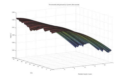
Figure 1. Simulated Yields in the generic affine class driven by CIR

3.4. Pricing formula of Swaptions

The pay-off (at its maturity $T_{\alpha}$) of a (unit of) swaption is

(3.5) $$(S_{\alpha,\beta}(T_{\alpha})-K)^{+}\sum_{i=\alpha+1}^{\beta}\tau_{i}P(T_{\alpha},T_{i}),$$

where $\{T_{\alpha},T_{\alpha+1},\ldots,T_{\beta}\}$ with $\tau_{i}=T_{i}-T_{i-1}$ is the tenor structure of the swap contract, and

$$S_{\alpha,\beta}(T_{\alpha})=\frac{1-P(T_{\alpha},T_{\beta})}{\sum_{i=\alpha+1}^{\beta}\tau_{i}P(T_{\alpha},T_{i})}$$

is the swap rate (see e.g. (Brigo and Mercurio, 2006)*Chapter 1, section 6). Note that (3.5) can be rewritten as

(3.6) $$\{1-P(T_{\alpha},T_{\beta})-K\sum_{i=\alpha+1}^{\beta}\tau_{i}P(T_{\alpha},T_{i})\}^{+}.$$

Therefore in the state price density approach, the quantity

$$\mathbf{sw}_{t}:=\frac{1}{\pi_{t}}E(\pi_{T_{\alpha}}\{1-P(T_{\alpha},T_{\beta})-K\sum_{i=\alpha+1}^{\beta}\tau_{i}P(T_{\alpha},T_{i})\}^{+}|\mathcal{F}_{t})$$

gives a fair price of the swaption. Substituting

$$P(T_{\alpha},T_{i})=E(\pi_{T_{i}}|\mathcal{F}_{T_{\alpha}})/\pi_{T_{\alpha}},$$

we get

$$\mathbf{sw}_{t}=\frac{1}{\pi_{t}}E(\{\pi_{T_{\alpha}}-E(\pi_{T_{\beta}}|\mathcal{F}_{T_{\alpha}})-K\sum_{i=\alpha+1}^{\beta}\tau_{i}E(\pi_{T_{i}}|\mathcal{F}_{T_{\alpha}})\}^{+}|\mathcal{F}_{t}).$$

By HKA, namely

$$\pi_{t}=p(t,X_{t}),$$

where $p$ has the propagation property w.r.t. a Markov process $X$. We have

(3.7) $$\begin{split}\mathbf{sw}_{t}&=\frac{1}{p(t,X_{t})}\times\\ &\quad\times E^{X_{t}}[\{p({T_{\alpha}},X_{T_{\alpha}-t})-p(2T_{\beta}-T_{\alpha},X_{T_{\alpha}-t})-\\ &\qquad-K\sum_{i=\alpha+1}^{\beta}\tau_{i}p(2T_{i}-T_{\alpha},X_{T_{\alpha}-t})\}^{+}],\end{split}$$

which is again – up to integration with respect to the law of $X$ – explicit.

3.5. Relations to short rate models

Assume that $p(t,x)$ is differentiable with respect to $t$. Then the short rate $R_{t}=-\partial_{T}\log P^{T}_{t}|_{t=T}$ of the previous interest rate model is given through

$$R_{t}=-\frac{1}{p(t,X^{x}_{t})}\frac{\partial}{\partial t}p(t,X^{x}_{t}).$$

Since $p>0$ the sign of the short rate is determined through

$$-\frac{\partial}{\partial t}p(t,X^{x}_{t}).$$

Notice that we do not necessarily have a short rate process.

3.6. Eigenfunction models

Take a finite dimensional manifold $M$ and take $X$ a Markov process with values in $M$. A non-vanishing function $g:M\to\mathbb{R}$ with

(3.8) $$E(g(X^{x}_{t}))=\exp(\mu t)g(x)$$

for some $\mu\leq 0$ is called eigenfunction of $X$. Let $g_{i}:M\to\mathbb{R}$, $i=1,\cdots,N$ be eigenfuntions with eigenvalues $\mu_{i}<0$, and let $A_{i}:\mathbb{R}_{\geq 0}\to\mathbb{R}_{>0}$ be decreasing functions. Set

$$v(t,x):=\sum_{i=1}^{N}A_{i}(t)g_{i}(x),$$

then we notice that $v(t,X_{t})$ is a supermartingale, too. If $v$ is strictly positive and $N>1$, then we can construct an arbitrage-free positive interest rate model by setting $\pi_{t}:=v(t,X_{t})$ as a state price density. We call such models the eigenfunction models.

Remark 3.5.

The class includes the generic approach II in the potential approach by Rogers (Rogers, 1997), and is included in the Flesaker-Hughston’s general framework since $e^{-\mu t}g(X_{t})$ becomes a martingale (see section 2.2).

3.7. Swaption Formula via eigenfunction models

The formula (3.7) becomes extremely simple when we use the eigenfunction model.

(3.9) $$\pi_{t}=p(t,X^{x}_{t})=1+e^{\mu t}g(X^{x}_{t})$$

where $g$ satisfies (3.8). By applying (3.9) on (3.7), we obtain the following result.

Theorem 3.6.

The pricing formula of the swaption is

$$\mathbf{sw}_{t}=\frac{1}{1+e^{\mu t}g(X^{x}_{t})}\int_{M}(Ag(y)-B)^{+}\,P(X_{T_{\alpha}-t}^{x}\in dy\,|\,x=X^{x}_{t}),$$

where

$$A=e^{\mu{T_{\alpha}}}-e^{\mu(2T_{\beta}-T_{\alpha})}-K\sum_{i=\alpha+1}^{\beta}\tau_{i}e^{\mu({T_{i}}+T_{\beta}-T_{\alpha})},$$

and

$$B=K(T_{\beta}-T_{\alpha}).$$

Example 3.7 (Brownian motion with drift).

Let $X$ be a Brownian motion with drift: whose generator is ${\Delta}/2-\kappa\cdot\nabla$ where $\kappa\in\mathbb{R}^{d}$. For $g(x)=e^{\langle c,x\rangle}$ with $c\in\mathbb{R}^{d}$, we have

$$({\Delta}/2-\kappa\cdot\nabla)g=(|c|^{2}/2-\langle\kappa,c\rangle)g.$$

Therefore, if $c$ is such that $|c|^{2}/2-\langle\kappa,c\rangle<0$ (this is always possible, take $c=\kappa$ for example), then the state price density

$$p(t,X_{t})=1+e^{\nu t}g(X_{t}),$$

where $\nu:=|c|^{2}/2-\langle\kappa,c\rangle$, gives a positive rate model. In this case

$$\begin{split}&\mathbf{sw}_{t}=\frac{1}{1+e^{\mu t}e^{\langle c,X_{t}^{x}\rangle}}{\bf BS}\Bigl{(}Ae^{\langle c,X^{x}_{t}\rangle},B,|c|\sqrt{T_{\alpha}-t},\langle c,\kappa\rangle\sqrt{T_{\alpha}-t}\Bigr{)},\end{split}$$

where

$${\bf BS}(a,b,c,d)=\frac{1}{\sqrt{2\pi}}\int_{\mathbb{R}}(ae^{cx+d}-b)^{+}e^{-\frac{x^{2}}{2}}\,dx.$$

Notice that the Black-Scholes formula for the price at time $t$ of the call option with the strike $K$ and the maturity $T$ is given by

$$e^{-r(T-t)}{\bf BS}(S_{t},K,\sigma\sqrt{T-t},(r-\frac{\sigma^{2}}{2})(T-t)).$$

Remark 3.8.

This example corresponds to the Flesaker-Hughston’s rational log-normal model (Flesaker and Hughston, 1992).

Example 3.9 (squared OU process).

Let $X$ be an Ornstein-Uhlenbeck process on ${\mathbb{R}}^{d}$, whose generator $\mathcal{A}$ is given by

$$\mathcal{A}:=-\mu x\nabla+\frac{1}{2}{\Delta}$$

where $\mu<0$. Setting $g(x)=e^{\mu|x|^{2}}$, we have

$$\mathcal{A}\,g(x)=\mu d\,g(x)$$

Therefore we have that $g$ is an eigenfunction with the eigenvalue ${\mu}d$. Setting $d=1$ and $p(t,x)=1+e^{\mu t}g(x)$, we obtain

(3.10) $$\begin{split}&\mathbf{sw}_{t}=\frac{Ae^{\mu(T_{\alpha}-t)}g(X^{x}_{t})\{\Phi(d_{1}^{+})-\Phi(d^{-}_{1})\}-B\{\Phi(d_{2}^{+})-\Phi(d_{2}^{-})\}}{1+e^{\mu t}g(X^{x}_{t})},\end{split}$$

where $\Phi(x)=\int_{-\infty}^{x}\frac{e^{-\frac{x^{2}}{2}}}{\sqrt{2\pi}}\,dx$,

(3.11) $$d_{1}^{\pm}=\frac{\pm\sqrt{\frac{1}{\mu}\log\frac{B}{A}}-X^{x}_{t}e^{\mu(T_{\alpha}-t)}}{\sqrt{(2\mu)^{-1}(e^{2\mu(T_{\alpha}-t)}-1)}}$$

and

(3.12) $$d_{2}^{\pm}=\frac{\pm\sqrt{\frac{1}{\mu}\log\frac{B}{A}}-X^{x}_{t}e^{-\mu(T_{\alpha}-t)}}{\sqrt{(2\mu)^{-1}(1-e^{-2\mu(T_{\alpha}-t)})}}.$$

For the proof see the Appendix 5.

4. HKA and Positive Rate Models

As we have pointed out the propagation property of $p$ does not ensure that the process $p(t,X_{t})$ is a supermartingale. Thus, the interest rate model with $\pi_{t}=p(t,X_{t})$ does not exclude the possibility of negative rates. In this section we provide models based on HKA and leading to positive short rates.

4.1. Weighted heat kernel approach

Let $p$ be a positive function with propagation property with respect to a Markov process $X$, and a weight $f:{\mathbb{R}}_{\geq 0}\times{\mathbb{R}}_{\geq 0}\to{\mathbb{R}}_{>0}$ such that $f(t,u-s)\leq f(t-s,u)$ for arbitrary $t,u\in{\mathbb{R}}_{\geq 0}$ and $s\leq t\wedge u$. Set

$$q(t,x)=\int_{0}^{\infty}p(s,x)f(t,s)\,ds,$$

Then we have

Proposition 4.1.

The process $q(t,X_{t})$ is a supermartingale.

Proof.

For $t>s$ and $x\in S$, we have

$$\begin{split}E(q(t,X^{x}_{t})|\mathcal{F}_{s})&=\int_{0}^{\infty}E(p(u,X^{x}_{t})|\mathcal{F}_{s})f(t,u)\,du\\ &=\int_{0}^{\infty}p(u+t-s,X^{x}_{s})f(t,u)\,du\\ &=\int_{t-s}^{\infty}p(v,X^{x}_{s})f(t,v-t+s)\,dv\end{split}$$

Here we have used the propagation property of $p$. Since

$$\begin{split}\int_{t-s}^{\infty}p(v,X^{x}_{s})f(t,v-t+s)\,dv&\leq\int_{t-s}^{\infty}p(v,X^{x}_{s})f(t-(t-s),v)\,dv\\ &\leq\int_{0}^{\infty}p(v,X^{x}_{s})f(s,v)\,dv=q(s,X_{s}^{x}),\end{split}$$

we have the desired result. ∎

Thus interest rate models with $\pi_{t}=q(t,X_{t})$ have positive short rates. The class is an extension of the potential models defined in (Rogers, 2006), since we can take $p$ as in (3.3) and $f(t,s)=e^{-\alpha(t+s)}$.

4.2. Killed Heat kernel approach

Let $V$ be a non-negative, measurable function defined on $S$. Put

$$q(t,x)=E(\exp{(-\int_{0}^{t}V(X^{x}_{s})\,ds)}),$$

and

(4.1) $$P_{t}^{T}=\frac{q(2T-t,X^{x}_{t})}{q(t,X^{x}_{t})}.$$

Then the bond market spanned by $P^{T}$ is arbitrage-free with respect to the state price density

$$\pi_{t}=q(t,X^{x}_{t})\exp(-\int_{0}^{t}V(X^{x}_{s})\,ds).$$

Indeed, this corresponds to an additional factor $Y_{t}^{y}=y+\int_{0}^{t}V(X^{x}_{s})\,ds$ for $y\geq 0$ added to the Markov process $X$. Since $(X^{x},Y^{y})$ is again a Markov process on $S\times\mathbb{R}_{\geq 0}$, we notice that

$$p(t,x,y):=E(e^{-Y^{y}_{t}})=e^{-y}E(\exp{(-\int_{0}^{t}V(X^{x}_{s})\,ds)})=e^{-y}q(t,x)$$

defined on $\mathbb{R}_{\geq 0}\times S\times\mathbb{R}_{\geq 0}$ satisfies the propagation property. Therefore the previously described bond prices are arbitrage-free with respect to the stated state price densities for initial values $(x,0)$. Since $q$ is decreasing in $t$ the short rates are again positive.

4.3. Trace approach

We give a third, more involved method to obtain positive rate models. Though it is only valid for symmetric Lévy processes at this stage, again the class is completely new. Let ${(X_{t})}_{t\geq 0}$ be a $d$-dimensional Lévy process, which is symmetric in the sense that $X_{1}\overset{\mathrm{d}}{=}-X_{1}$. We define $X^{x}_{t}=x+X_{t}$. Note that in this case its Lévy symbol is positive and symmetric, i.e.

$${E}(e^{2\pi i\langle\xi,X_{t}^{0}\rangle})=e^{-t\psi(\xi)}$$

for some

$$\psi:\mathbb{R}^{d}\to\mathbb{R}_{\geq 0},$$

which is symmetric in the sense that $\psi(\xi)=\psi(-\xi)$.

Let $\mu$ be a measure on $\mathbb{R}^{d}$ such that

$$\mu(-A)=\mu(A)$$

for any Borel set $A$. Put

$$u(t,x)=\int_{\mathbb{R}^{d}}e^{2\pi i\langle\eta,x\rangle}e^{-t\psi(\eta)}\mu(d\eta),$$

assuming it is finite (except at $t=0$) for each $x\in\mathbb{R}^{d}$.

Lemma 4.2.

The function $u$ is non-negative and has the propagation property with respect to $\{X^{x}\}$.

Proof.

First, notice that by the symmetry of $\mu$ we have

(4.2) $$u(t,x)=\int_{\mathbb{R}^{d}}\cos(2\pi\langle\eta,x\rangle)e^{-t\psi(\eta)}\mu(d\eta)\in\mathbb{R},$$

and $u(t,x)=u(t,-x)$ for any $x\in\mathbb{R}^{d}$. Then by Bochner’s theorem we know that $u(t,\cdot)$ is non-negative definite and we see that $u(t,x)\geq 0$ for any $x\in\mathbb{R}^{d}$.

Since $|u_{t}(x)|\leq 1$, $\mathbf{E}[u(s,X^{x}_{t})]\leq 1$ for any $s,t>0$ and $x\in\mathbb{R}^{d}$, we have

$$\begin{split}E(u(s,X^{x}_{t}))&=E\left(\int_{\mathbb{R}^{d}}e^{2\pi i\langle\eta,X_{t}^{x}\rangle}e^{-s\psi(\eta)}\mu(d\eta)\right)\\ &=\int_{\mathbb{R}^{d}}{E}(e^{2\pi i\langle\eta,X_{t}^{x}\rangle})e^{-s\psi(\eta)}\mu(d\eta)\\ &=\int_{\mathbb{R}^{d}}e^{2\pi i\langle\eta,x\rangle}E(e^{2\pi i\langle\eta,X_{t}^{0}\rangle})e^{-s\psi(\eta)}\mu(d\eta)\\ &=\int_{\mathbb{R}^{d}}e^{2\pi i\langle\eta,x\rangle}e^{-(s+t)\psi(\eta)}\mu(d\eta)=u(t+s,x).\end{split}$$

∎

Remark 4.3.

If the Fourier transform

$$f(x):=\int_{\mathbb{R}^{d}}e^{2\pi i\langle x,\xi\rangle}\mu(d\xi)$$

exists and is bounded in $x$, then by the symmetry of $\mu$ it holds that $f(x)\geq 0$, and $u$ has the following expression:

$$u(t,x)=E(f(X^{x}_{t})).$$

On the other hand, let $\mu$ be the Lebesgue measure of $\mathbb{R}^{d}$. If the density $p_{t}(x)$ of $X^{0}_{t}$ exists in $L^{1}\cap L^{2}$, we have

$$u(t,x)=p_{t}(x).$$

That is, $u$ is the heat kernel.

We are now able to prove the following theorem on supermartingales constructed from heat kernels:

Theorem 4.4.

Let $c$ be a positive constant greater than $2$ and let $\lambda$ be any positive constant. Set $\pi_{t}:=u(\lambda+t,X^{x}_{t})+cu(\lambda+t,0)$. Then $\pi$ is a supermartingale with respect to the natural filtration of $X$.

Proof.

By the expression (4.2), we have

(4.3) $$\begin{split}&u(\lambda+t,X^{x}_{t})-u(\lambda+2T-t,X^{x}_{t})\\ &\hskip 56.9055pt=\int_{\mathbb{R}^{d}}\cos 2\pi\langle X^{x}_{t},\xi\rangle(e^{-(t+\lambda)\psi(\xi)}-e^{-(\lambda+2T-t)\psi(\xi)})\mu(d\xi)\end{split}$$

Since $\psi\geq 0$ and $\lambda$ is positive,

RHS of (4.3)

$$\geq\int_{\mathbb{R}^{d}}(e^{-(t+\lambda)\psi(\xi)}-e^{-(\lambda+2T-t))\psi(\xi)})\mu(d\xi)$$

$$=-(u(t+\lambda,0)-u(\lambda+2T-t,0)).$$

Thus we obtain

$$u(t+\lambda,X^{x}_{t})+u(t+\lambda,0)$$

$$\hskip 56.9055pt\geq u(\lambda+2T-t,X^{x}_{t})+u(\lambda+2T-t,0),$$

and then

(4.4) $$\begin{split}&u(t+\lambda,X^{x}_{t})+cu(t+\lambda,0)\\ &\geq u(\lambda+2T-t,X^{x}_{t})+u(\lambda+2T-t,0)+(c-1)u(t+\lambda,0).\end{split}$$

On the other hand, by an elementary inequality we have

$$u(\lambda+2T-t,0)+u(t+\lambda,0)$$

$$=\int_{\mathbb{R}^{d}}(e^{-(\lambda+2T-t)\psi(\xi)}+e^{-(t+\lambda)\psi(\xi)})\mu(d\xi)$$

$$\geq 2\int_{\mathbb{R}^{d}}e^{-\frac{1}{2}(\lambda+\lambda+2T)\psi(\xi)}\mu(d\xi),$$

and since $\lambda$ is positive, we obtain

(4.5) $$\begin{split}&u(\lambda+2T-t,0)+u(t+\lambda,0)\\ &\hskip 56.9055pt\geq 2\int_{\mathbb{R}^{d}}e^{-(T+\lambda)\psi(\xi)}\mu(d\xi)=2u(T+\lambda,0).\end{split}$$

Combining (4.4) and (4.5), we have

(4.6) $$\begin{split}&u(t+\lambda,X^{x}_{t})+cu(t+\lambda,0)-\\ &\qquad-u(\lambda+2T-t,X^{x}_{t})-cu(T+\lambda,0)\\ &\hskip 56.9055pt\geq(c-2)(u(t+\lambda,0)-(c-2)u(T+\lambda,0)).\end{split}$$

The right-hand-side of (4.6) is non-negative since $c\geq 2$ and

$$u(t,0)=\int_{\mathbb{R}^{d}}e^{-t\psi(\xi)}\,\mu(d\xi)$$

is decreasing in $t$. Finally, since we have

$$E[\pi_{T}|\mathcal{F}_{t}]=u(\lambda+2T-t,X^{x}_{t})+cu(T+\lambda,0),$$

we now see that $\pi_{t}$ is a supermartingale. ∎

4.4. Examples

By the above theorem, we can now construct a positive interest rate model by setting $u(\lambda+2T-t,X^{x}_{t})+cu(T+\lambda,0)$ to be a state price density, or equivalently

$$P^{T}_{t}=\frac{u(\lambda+2T-t,X^{x}_{t})+cu(T+\lambda,0)}{u(t+\lambda,X^{x}_{t})+cu(t+\lambda,0)}.$$

Here we give some explicit examples. In all examples, $c$ is a constant greater than $2$ and $\lambda$ some positive constant.

Example 4.5 (Heat Kernel with Trace).

A simple example is obtained by letting

$$u(t,x)=\frac{1}{\sqrt{2\pi t}}e^{-\frac{x^{2}}{2t}},$$

where the bond prices are expressed as

$$P^{T}_{t}=\frac{\sqrt{\frac{\lambda+t}{\lambda+2T-t}}e^{-\frac{W^{2}_{t}}{\lambda_{T}+2T-t}}+\sqrt{\frac{\lambda+t}{\lambda+T}}c}{e^{-\frac{W^{2}_{t}}{\lambda+t}}+c}$$

Example 4.6 (Quadratic Gaussian with Trace).

A similar model can be obtained by setting, for $\alpha>0$,

$$\begin{split}u(t,x)&=\frac{1}{\sqrt{(t\alpha^{2}+1)}}e^{-\frac{\alpha^{2}}{2(t\alpha^{2}+1)}x^{2}}\\ &\left(=E_{x}(e^{-\frac{\alpha^{2}}{2}W^{2}_{t}})=E\left(\int_{\mathbb{R}}e^{iy\alpha W_{t}^{x}}\frac{1}{\sqrt{2\pi}}e^{-\frac{y^{2}}{2}}\,dy\right)\right).\end{split}$$

A visualization of this model is shown in Figure 2.

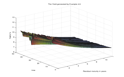
Figure 2. Simulated Yields for the trace class model driven by a Quadratic Gaussian

Example 4.7 (Cauchy $0$ with Trace).

Let $Z^{x}$ be a Cauchy process in ${\mathbb{R}}^{d}$ starting from $x$. The explicit form of the transition density of $Z^{0}$ is known to be

(4.7) $$p(t,x):=\frac{\Gamma((d+1)/2)\theta t}{(\pi\{(\theta t)^{2}+|x-t\gamma|^{2}\})^{(d+1)/2}},$$

where $\theta>0$ and $\gamma\in{\mathbb{R}}^{d}$ (see e.g.(Sato, 1999)). Note that Cauchy processes are strictly stable (or self-similar) process with parameter $1$; namely,

$$Z_{at}\overset{\mathrm{d}}{=}aZ_{t},\quad a>0,t>0.$$

This property is seen from their Lévy symbol: actually we have

$${E}[e^{i\langle\xi,Z_{t}\rangle}]=e^{-t(\theta|\xi|-i\langle\xi,\gamma\rangle)}.$$

If we set $\gamma=0$, the density turns symmetric and therefore, setting $\pi_{t}=p(\lambda+t,Z^{x}_{t})+cp(\lambda+t,0)$, we obtain an explicit positive term structure model. We give the explicit form of the bond prices in the case of $d=1$:

$$\begin{split}P^{T}_{t}&=\frac{\lambda+t}{\lambda+2T-t}\frac{\theta^{2}(\lambda+t)^{2}+|Z^{x}_{t}|^{2}}{\theta^{2}(\lambda+2T-t)^{2}+|Z^{x}_{t}|^{2}}\\ &\hskip 56.9055pt\times\frac{\theta^{2}(1+c)(\lambda+2T-t)^{2}+c|Z^{x}_{t}|^{2}}{\theta^{2}(1+c)(\lambda+t)^{2}+c|Z^{x}_{t}|^{2}}.\end{split}$$

The model is a modification of the Cauchy TSMs given in (Akahori and Tsuchiya, 2006).

Let $X_{t}$ be Lévy process and $T_{t}$ be a subordinator independent of $X_{t}$. Recall that the process $Z_{t}:=X_{T_{t}}$ is usually called the subordination of $X$ by the subordinator $T$. Among the subordinations of the Wiener process, two classes are often used in the financial context; one is the Variance Gamma processes and the other is Normal Inverse Gaussian processes, since they are analytically tractable (see (Rama Cont, 2004) and references therein). The subordinator of a Variance Gamma process (resp. Normal Inverse Gaussian process) is a Gamma process (resp. Inverse Gaussian process). If we let the drift of the Wiener process be zero, then the densities of the subordinated processes satisfies the condition for Theorem 4.4.

Example 4.8 (Variance Gamma TSMs with Trace).

The Gamma subordinator $T^{G}$ is a Lévy process with

$$P(T^{G}_{t}\in dx)/dx=\frac{\gamma^{\eta t}}{\Gamma(\eta t)}x^{\eta t-1}e^{-\gamma x}1_{\{x\geq 0\}},$$

where $\eta$ and $\gamma$ are positive constants. Then the heat kernel of the subordinated Wiener process $W_{T_{t}^{G}}$ is

(4.8) $$u(t,x):=\int_{0}^{\infty}\frac{1}{\sqrt{2\pi s}}e^{-\frac{x^{2}}{2s}}\frac{\gamma^{\eta t}}{\Gamma(\eta t)}s^{\eta t-1}e^{-\gamma s}\,ds.$$

From this expression we have

$$u(t,0)=\sqrt{\frac{\gamma}{2\pi}}\frac{\Gamma(\eta t-\frac{1}{2})}{\Gamma(\eta t)}.$$

The heat kernel (4.8) can be expressed in terms of the modified Bessel functions $K_{p}$, $p\in\mathbb{R}$, which has an integral representation

(4.9) $$K_{p}(x)=\frac{1}{2}\left(\frac{x}{2}\right)^{p}\int_{0}^{\infty}e^{-t-\frac{x^{2}}{4t}}t^{-p-1}\,dt,\quad x>0.$$

Actually we have

$$u(t,x)=\sqrt{\frac{2}{\pi}}\Gamma(\eta t)^{-1}\left(\frac{\gamma}{2}\right)^{-\frac{\eta t}{2}+\frac{1}{4}}|x|^{-\eta t+\frac{1}{2}}K_{-\eta t+\frac{1}{2}}\left(|x|\sqrt{2\gamma}\right).$$

Example 4.9 (Normal Inverse Gaussian TSMs with Trace).

The heat kernel of the inverse Gaussian subordinator $T^{I}_{t}$ is

$$\rho_{t}(x):=\frac{\eta t}{x^{3/2}}e^{2\eta t\sqrt{\pi\gamma}}e^{-\gamma x-\pi\eta^{2}t^{2}/x},\quad x>0,$$

where $\eta$ and $\gamma$ are positive constants. The heat kernel of the subordinated Wiener process $W_{T^{I}_{t}}$ is

$$u(t,x):=\int_{0}^{\infty}\frac{1}{\sqrt{2\pi s}}e^{-\frac{x^{2}}{2s}}\rho_{t}(s)\,ds.$$

Applying (4.9), we obtain

$$u(t,x)=\frac{1}{2\pi}\frac{\eta t}{y{\gamma}^{3}}e^{2\eta t\sqrt{\pi\gamma}}K_{1}\left(\sqrt{\gamma(2x^{2}+4\pi\eta^{2}t^{2})}\right).$$

In particular, we have

$$u(t,0)=\frac{1}{2\pi}\frac{\eta t}{y_{0}{\gamma}^{3}}e^{2\eta t\sqrt{\pi\gamma}}K_{1}\left(2\eta t\sqrt{\gamma\pi}\right).$$

5. Appendix

Lemma 5.1.

For $m,a,b\in\mathbb{R}$, $v>0$, and $\mu<0$, it holds

(5.1) $$\begin{split}&\int_{a\leq x\leq b}e^{\mu x^{2}}\frac{1}{\sqrt{2\pi v}}e^{-\frac{(x-m)^{2}}{2v}}dx\\ &=\sqrt{\frac{\tilde{v}}{v}}e^{\frac{\mu m^{2}}{1-2\mu v}}\left(\Phi(\frac{b-\tilde{m}}{\sqrt{\tilde{v}}})-\Phi(\frac{a-\tilde{m}}{\sqrt{\tilde{v}}}).\right)\end{split}$$

where

(5.2) $$\tilde{m}:=\frac{m}{1-2\mu v}\ \ {\rm and}\ \ \tilde{v}:=\frac{v}{1-2\mu v}.$$

Proof.

(5.3) $$\begin{split}&\int_{a\leq x\leq b}e^{\mu x^{2}}\frac{1}{\sqrt{2\pi v}}e^{-\frac{(x-m)^{2}}{2v}}dx\\ &=\sqrt{\frac{\tilde{v}}{v}}e^{\frac{\mu m^{2}}{1-2\mu v}}\int_{a\leq x\leq b}\frac{1}{\sqrt{2\pi\tilde{v}}}e^{-\frac{(x-\tilde{m})^{2}}{2\tilde{v}}}dx\\ &=\sqrt{\frac{\tilde{v}}{v}}e^{\frac{\mu m^{2}}{1-2\mu v}}\left(\Phi(\frac{b-\tilde{m}}{\sqrt{\tilde{v}}})-\Phi(\frac{a-\tilde{m}}{\sqrt{\tilde{v}}})\right).\end{split}$$

∎

A proof of (3.10) with (3.11) and (3.12)

Notice that

(5.4) $$X_{T_{\alpha}-t}\big{|}_{X_{t}}\sim N(m_{t},v_{t})$$

where

(5.5) $$m=X_{t}e^{-\mu(T_{\alpha}-t)}\ \ \text{and}\ \ v=\frac{1}{2\mu}(1-e^{-2\mu(T_{\alpha}-t)}).$$

Put

$$a=-\sqrt{\frac{1}{\mu}\log\frac{B}{A}}\ \ {\rm and}\ \ b=\sqrt{\frac{1}{\mu}\log\frac{B}{A}}.$$

By Lemma 5.1, we have

(5.6) $$\begin{split}&\int_{\mathbb{R}}(Ag(y)-B)^{+}P(X_{T_{\alpha}-t}^{x}\in dy\ |\ x=X_{t})\\ &=A\sqrt{\frac{\tilde{v}}{v}}e^{\frac{\mu m^{2}}{1-2\mu v}}\left(\Phi(\frac{b-\tilde{m}}{\sqrt{\tilde{v}}})-\Phi(\frac{a-\tilde{m}}{\sqrt{\tilde{v}}}).\right)-B\left(\Phi(\frac{b-m}{\sqrt{v}})-\Phi(\frac{a-m}{\sqrt{v}})\right).\end{split}$$

By (5.2) and (5.5)

$$\tilde{m}=X_{t}e^{\mu(T_{\alpha}-t)},\quad\tilde{v}=\frac{e^{2\mu(T_{\alpha}-t)}-1}{2\mu},$$

$$e^{\frac{\mu m^{2}}{1-2\mu v}}=e^{\mu|X_{t}^{x}|^{2}}=g(X_{t}^{x}),$$

and

$$\sqrt{\tilde{v}/v}=(1-2\mu v)^{-1/2}=e^{\mu(T_{\alpha}-t)}.$$

With these expression we have (3.10). ∎

References

- (1)
- Akahori and Hara (2006) Akahori, Jirô and Kesuke Hara, “Lifting quadratic term structure models to infinite dimension,” Mathematical Finance, 2006, 16 (4), 635–645.
- Akahori and Tsuchiya (2006) by same author and Takahiro Tsuchiya, “What is the natural scale for a Lévy process in modelling term structure of interest rates?,” Asia-Pacific Financial Markets, 2006, 13 (4), 299–313.
- Brigo and Mercurio (2006) Brigo, Damiano and Fabio Mercurio, Interest Rate Models - Theory and Practice: With Smile, Inflation and Credit (Springer Finance), Springer, September 2006.
- Rama Cont (2004) Cont, Peter Tankov Rama, Financial modelling with jump processes Chapman & Hall/CRC Financial Mathematics Series, Chapman & Hall/CRC, Boca Raton, FL, 2004.
- Flesaker and Hughston (1992) Flesaker, Bjorn and L.P. Hughston, “Positive Interest,” Risk Magazine, 1992, 9 (1), 46–49.
- Grasselli and Hurd. (2003) Grasselli, M. R. and T. R. Hurd., “Wiener Chaos and the Cox-Ingersoll-Ross model,” 2003.
- Heath et al. (1992) Heath, David, Robert Jarrow, and Andrew Morton, “Bond pricing and the term structure of interest rates: a new methodology for contingent claims valuation,” Econometrica, 1992, 60 (1), 77–105.
- Lane P. Hughston (2005) Hughston, Avraam Rafailidis Lane P., “A chaotic approach to interest rate modelling,” Finance and Stochastics, 2005, 9 (1), 43–65.
- Hunt et al. (2000) Hunt, Phil, Joanne Kennedy, and Antoon Pelsser, “Markov-functional interest rate models,” Finance and Stochastics, 2000, 4 (4), 391–408.
- Rogers (1997) Rogers, L. C. G., “The potential approach to the term structure of interest rates and foreign exchange rates,” Math. Finance, 1997, 7 (2), 157–176.
- Rogers (2006) by same author, “One for all: the potential approach to pricing and hedging,” 2006, 8, 407–421.
- Sato (1999) Sato, Keniti, Lévy processes and infinitely divisible distributions, Vol. 68 of Cambridge Studies in Advanced Mathematics, Cambridge University Press, 1999. Translated from the 1990 Japanese original; Revised by the author.
- Shirakawa (1991) Shirakawa, Hiroshi, “Interest rate option pricing with Poisson-Gaussian forward rate curve processes,” Math. Finance, 1991, 1 (1), 77–94.