A Large Scale Survey of X-Ray Filaments in the Galactic Center

Abstract

We present a catalog of 17 filamentary X-ray features located within a 68’$\times$34’ view centered on the Galactic Center region from images taken by Chandra. These features are described by their morphological and spectral properties. Many of the X-ray features have non-thermal spectra that are well fit by an absorbed power-law. Of the 17 features, we find 6 that have not been previously detected, 4 of which are outside the immediate 20’$\times$20’ area centered on the GC. 7 of the 17 identified filaments have morphological and spectral properties expected for pulsar wind nebulae with X-ray luminosities of 5$\times$10³² to 10³⁴ ergs s^-1 in the 2.0-10.0 keV band and photon indexes in the range of $\Gamma$=1.1 to 1.9. In one feature, we suggest the strong neutral Fe K$\alpha$ emission line to be a possible indicator for past activity of Sgr A*. For G359.942-0.03, a particular filament of interest, we propose the model of a ram-pressure confined stellar wind bubble from a massive star to account for the morphology, spectral shape and 6.7 keV He-like Fe emission detected. We also present a piecewise spectral analysis on two features of interest, G0.13-0.11 and G359.89-0.08, to further examine their physical interpretations. This analysis favors the PWN scenario for these features.

1 Introduction

The Galactic Center (GC) region is a unique environment that is home to numerous energetic processes. Radio, infrared and X-ray observations show structures that can only be distinguished in our own galaxy due to its proximity. The GC thus provides a laboratory in which to probe the Galactic nuclear environment and the interactions between star formation regions, the interstellar medium (ISM) and the supermassive black hole Sgr A*. These observations can aid in understanding the nuclear environments of nearby galaxies.

Radio observations have detected prominent non-thermal radio filaments that have been intensively studied (e.g. Yusef-Zadeh, Morris & Chance, 1984). Many of the non-thermal radio filaments may come from milliGauss magnetic fields illuminated by energetic particles. These fields are seen to be primarily perpendicular to the galactic plane and indicate the general structure of the magnetic field around the GC. The exact origins and implications of the radio non-thermal filaments in relation to the GC are still in debate.

Chandra observations have detected numerous large scale X-ray structures from thermal to non-thermal filaments (e.g. Bamba et al., 2002; Lu, Yuan, & Lou, 2008; Muno et al., 2007) primarily in the local 20’$\times$20’ area centered on the GC. The commonly accepted scenarios for non-thermal thread-like X-ray features in the GC include pulsar wind nebulae (PWNe) (e.g. Wang, Li, & Begelman, 1993; Wang, Lu & Gotthelf, 2006), with the filament-like structure produced through ram-pressure confinement or strong magnetic fields, and magnetohydrodynamical shock fronts from supernova remnants (SNRs) (e.g Yusef-Zadeh et al., 2005). For the SNR case, the elongation of features represent shock fronts in the ISM. The average non-thermal spectrum of a typical PWN is generally well fit by a power law model with a photon index in the range of $\Gamma$=1.1-2.4 (Gotthelf & Olbert, 2002) and X-ray luminosities in the range of $10^{32}$ to $10^{37}$ ergs s^-1 for the 0.2-10 keV energy band (e.g. Gaensler & Slane, 2006; Kaspi, Roberts & Harding, 2006). The PWN scenario is motivated primarily by the similarities between the features seen in the GC and X-ray features associated with known pulsars (see also Kargaltsev & Pavlov, 2008). Few cases of K$\alpha$ transitions from neutral iron (Fe) are proposed to stem from the reflection of hard X-rays from external sources, such as the supermassive black hole Sgr A* (e.g. Koyama et al., 1989). By analyzing these X-ray features, one can in principle trace gas dynamics and magnetic fields in the GC region (e.g. Wang, Lu, & Lang, 2002) and examine the history of GC activity (Koyama et al., 1989).

Previous broad scale studies of X-ray features focus on the immediate 20’$\times$20’ area surrounding Sgr A* (e.g. Muno et al., 2007; Lu, Yuan, & Lou, 2008). Here, we present a wide scale study on 17 X-ray thread-like features. The features are detected over a roughly 68’$\times$34’ area of the sky, relating to approximately 158 pc by 79 pc, around Sgr A* based on all available observations. While some of these features have been examined in previous literature, the improved counting statistics of this study allows for piecewise analysis that will be able to detect trends in the spectra and therefore better constrain the physical model (see also Lu, Yuan, & Lou, 2008). In addition to the piecewise analysis of some features, we also present an additional physical model in order to explain a feature with a Helium (He)-like Fe K$\alpha$ emission line, comet-like morphology and steep spectrum. For consistency within this study, the spectral and morphological characteristics were performed for all features listed. All physical distance measurements assume an 8 kpc distance to the GC and all errors, unless otherwise stated, are given to the 90% confidence level.

2 Observations and Detection

The Chandra X-ray Observatory observed the GC with the Advanced CCD Imaging Spectrometer imaging array (ACIS-I) for a total integrated exposure time of $\sim$2 Msec between 1999 and 2007 over 81 observations (Muno et al., 2008). The array is composed of four individual CCDs that operate together to provide a 17’$\times$17’ view with sub-arcsecond resolution at the center of the array. The images were first reprocessed using the standard Chandra Interactive Analysis of Observations ciao routines (version 3.4.0) and then combined by celestial coordinates to produce a merged events file.

Initial identification of X-ray filaments comes from a careful visual examination of the merged event image in the 2.0-8.0 keV band. We examine the merged events file under a logarithmic scale with different upper/lower limits and look for extended, linear structures. From this initial identification, we removed features whose morphologies and apparent extended structures are not well confined with respect to the feature in question, leaving only those with tightly correlated extended X-ray emission. Within regions of strong diffuse X-ray emission, e.g. the Sgr A* complex, we limited our selection to well constrained extended X-ray emission regions with size scales larger than 3”$\times$1”. These morphologically selected features were culled once more after taking their individual spectra (see below for details on spectral extraction) and rejecting them if their spectra appear consistent with their local background; e.g. in spectral shape. Based on our selection criteria, these features are thus X-ray bright, in respect to their local backgrounds, and have well defined linear morphologies; however, due to the complexity of X-ray emission around the GC and the uneven sensitivity of this survey, this sample is far from complete and represents only a fraction of the extended X-ray features indigenous to the GC. Fig. 1 shows the composite intensity map in the 2.0-8.0 keV band with identified features labeled and indicated by their surrounding ellipses. Fig. 2 shows the inner 20’$\times$20’ around Sgr A* with features again labeled and constrained by their surrounding ellipses. In extracting their source and background spectra, point sources and other such possible contaminators were excluded from the count and exposure maps. We use local background subtraction for each filament due to the widespread area and time integration over which the filaments are found. For those that are surrounded by strong diffuse emission, e.g. within the Sgr A* complex, backgrounds were selected to account for the immediate intensities.

Figure 1: Full view of the 81 compiled observations taken by Chandra around the GC. The center square identifies the 20’$\times$20’ region of Fig. 2. Features outside this region are selected by their surrounding ellipses and labeled based on their galactic coordinates. The image is the exposure-corrected intensity map in the 2.0-8.0 keV band produced by dividing the ACIS-I count map with the exposure map. This and subsequent images are given in logarithmic scaling with North defined as up and East as left.

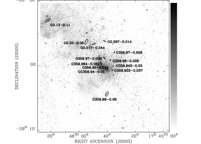
Figure 2: Magnified view of the intensity map from Fig.1 on the inner 20’$\times$20’ area centered on Sgr A*. Identified features are again selected and labeled by their surrounding ellipses.

Typical spectral extraction methods pose a problem for the features that were covered by multiple observations. While some of the 81 observations have the same celestial coordinates in their pointing, they could have different roll angles. As such, a feature could fall into different positions on the ACIS-I detector over different observations including the gap between the CCDs that compose the array. Additionally, a feature may be completely contained within one observation while partially covered in another. Therefore, the traditional spectral extraction could not be used due to time and spatial variability of the Auxiliary Response File (arf) and Redistribution Matrix File (rmf) of the instrument. Another way is to extract the spectra of the filaments from individual observations and use ”ftools” to merge them into a final spectrum. However, this is just suitable for a single object and can become difficult when dealing with many filaments over many observations. Therefore, we developed a new method to directly extract the spectrum from the merged events file. We first reproject all the events in the merged events file of a certain filament into the instrument coordinate, since the calculation of the arf and rmf is based on events’ positions on the CCD, not the celestial coordinate. The arf is not only a function of the events’ positions, but also depends on when the observation was taken. The quantum efficiency of the CCDs has been seen to degrade over time in part due to molecular contamination build up on the the CCD itself and/or the filter. However, we notice that above 2 keV, the arf of ACIS-I decreases less than 5% during the 7 years observational period (absorption towards the GC is large for energies below 2 keV, making the 2 keV lower limit optimal in terms of spectral analysis). Using this lower limit, the arf can then be considered to be time-independent. The rmf file is very stable and is just a function of position, not time (we have checked the rmf file used by the ciao routines for each observation one by one. All of them use the same calibration file). Therefore, a new response matrix file, rsp (the multiple of the arf and rmf file), for each small grid on the CCD (the place of each grid in the CCD is predefined by the calibration file) with events was created from the calibration file and the total number of events falling into each grid was used as the weight for merging all the new rsp files in different grids into the final merged rsp. We have tested this method in the center 7’ region around SGR A* and found that the fitting result from this method is nearly identical to that from the same region in the observation with the longest exposure time, proving that our method is robust and reliable.

3 Analysis of X-ray Features

For each of the identified filaments, we classify its basic appearance as well as spectral proprieties. We broadly classify the features into two morphological categories: ’filamentary’ and ’cometary’. A feature is considered to be cometary if its morphology appears to taper off in one direction, similar to a comet’s tail, or if it has apparent asymmetry in its brightness across its major axis. Features that do not meet these criteria are defined as filamentary, this includes features that appear to be brightest in the center. This morphological classification along with the sizes of the features are approximations based on the observed flux and apparent surface brightness relative to the local background. The name associated with each feature comes from the approximate center or brightest point of the feature.

Fig. 3 through 7 show the individual features with ellipses indicating regions used in extracting the source and background spectra. Linear X-ray features can be seen in some images in addition to the features identified. Many of these were either not selected due to the possibility of being small scale structures of a larger X-ray emitting region or rejected based on our selection criteria. The plot next to each Chandra count map gives the extracted spectrum for each feature. In each case, the spectrum is well fit using a power law model with foreground absorption in xspec (pha(po) for short). A Gaussian model is included for those features which exhibit line emission of 6.4 keV neutral Fe or 6.7 keV He-like Fe (pha(po+ga)). The spectral parameters for the pha(po) or pha(po+ga) single fit models as well as the morphological properties for the features are listed in Tables 1 and 2. It is well known that extinction towards the GC can vary greatly over scales on order of arc-seconds (e.g. Scoville et al., 2003). As such, each feature is modeled with an independent value of column density ($N_{\rm{H}}$) rather than a single fixed $N_{\rm{H}}$ for all features based on the assumed 8 kpc distance to the GC. The following summary of features focuses on those with unique traits or observations.

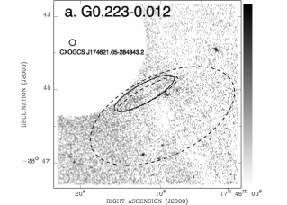
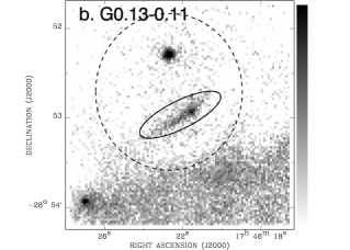
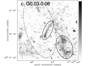
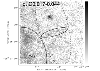
Figure 3: Left-hand panel: the X-ray count maps of individual features in the 2.0-8.0 keV band. The upper and lower limits for each count map are 12 and 0.5 counts/arcsec² for G0.223-0.012 (a), 23 and 2.3 counts/arcsec² for G0.13-0.11 (b), 69 and 6.9 counts/arcsec² for G0.03-0.06 (c), and 207 and 4.1 counts/arcsec² for G0.017-0.044 (d), respectively. Source regions are identified by the solid ellipses with background regions enclosed by dashed ellipses. In 3a, the empty region results from the removal of events around the bright X-ray point source CXOGCS J174621.05-284343.2 whose position is given by the small circular region. Fig. 3c and 3d include the ’West Clump’ region from Lu, Yuan, & Lou (2008), labeled as ’WC’. Right-hand panel: the X-ray spectra for the matching features given in the left column in the 2.0-8.0 keV band. All spectra are fit with an absorbed power-law model (pha(po)). The model for G0.017-0.044 is fitted with a Gaussian centered at 6.4 keV in addition to the pha(po)

figure=images/G0.007-0.014.ps,width=2.3in figure=images/G0.007-0.014_spec.ps,width=2.3in,angle=-90 figure=images/G359.97-0.038.ps,width=2.3in figure=images/G359.97-0.038_spec.ps,width=2.3in,angle=-90 figure=images/G359.97-0.009.ps,width=2.3in figure=images/G359.97-0.009_spec.ps,width=2.3in,angle=-90 figure=images/G359.964-0.052.ps,width=2.3in figure=images/G359.964-0.052_spec.ps,width=2.3in,angle=-90

Figure 4: Continued X-ray count maps and spectra similar to Fig. 3. Upper and lower limits for each count map are 103 and 4.1 counts/arcsec² for G0.007-0.014 (a), 410 and 4.1 counts/arcsec² for G359.97-0.038 (b), 207 and 4.1 counts/arcsec² for G359.97-0.009 (c), and 410 and 12 counts/arcsec² for G359.964-0.052 (d), respectively.

figure=images/G359.96-0.028.ps,width=2.3in figure=images/G359.96-0.028_spec.ps,width=2.3in,angle=-90 figure=images/G359.95-0.04.ps,width=2.3in figure=images/G359.95-0.04_spec.ps,width=2.3in,angle=-90 figure=images/G359.942-0.03.ps,width=2.3in figure=images/G359.942-0.03_spec.ps,width=2.3in,angle=-90 figure=images/G359.94-0.05.ps,width=2.3in figure=images/G359.94-0.05_spec.ps,width=2.3in,angle=-90

Figure 5: Continued X-ray count maps and spectra. Upper and lower limits for each count map are 207 and 8.3 counts/arcsec² for G359.96-0.028 (a), 1200 and 21 counts/arcsec² for G359.95-0.04 (b), 207 and 12 counts/arcsec² for G359.942-0.03 (c), and 410 and 4.1 count/arcsec² for G359.94-0.05 (d), respectively. G359.942-0.03 is fitted with a 6.7 keV Gaussian in addition to the pha(po) model.

figure=images/G359.933-0.037.ps,width=2.3in figure=images/G359.933-0.037_spec.ps,width=2.3in,angle=-90 figure=images/G359.89-0.08.ps,width=2.3in figure=images/G359.89-0.08_spec.ps,width=2.3in,angle=-90 figure=images/G359.55+0.16.ps,width=2.3in figure=images/G359.55+0.16_spec.ps,width=2.3in,angle=-90 figure=images/G359.43-0.14.ps,width=2.3in figure=images/G359.43-0.14_spec.ps,width=2.3in,angle=-90

Figure 6: Continued X-ray count maps and spectra. Upper and lower limits for each count map are 410 and 8.3 counts/arcsec² for G359.933-0.037 (a), 410 and 4.1 counts/arcsec² for G359.89-0.08 (b), and 12 and 0.5 counts/arcsec² for G359.55+0.16 (c) and G359.43-0.14 (d), respectively.

figure=images/G359.40-0.08.ps,width=2.3in figure=images/G359.40-0.08_spec.ps,width=2.3in,angle=-90

Figure 7: Final X-ray count map and spectra. The count map has upper and lower limits of 12 and 0.5 counts/arcsec².

figure=images/G0.13-0.11_dif.ps,width=2.3in

figure=images/G359.89-0.08_w.ps,width=2.3in figure=images/G359.89-0.08_l.ps,width=2.3in

Figure 8: Region selection for piecewise analyses. The count maps for G0.13-0.11 and G359.89-0.08 are overlaid with regions identifying the segments to be used in their respective piecewise analyses. The region selection for G0.13-0.11 is shown in 8a. The image 8b gives the minor axis selection for G359.89-0.08 while 8c gives the major axis selection.

3.1 G0.223-0.012

G0.223-0.012 (Fig. 3a) is located near the bright X-ray point source CXOGCS J174621.05-284343.2, removed from the image in Fig. 3a with its location marked, to the northeast of the feature. The feature’s position as well as orientation rejects the possibility that G0.223-0.012 could be the result of a CCD readout streak from CXOGCS J174621.05-284343.2.

3.2 G0.13-0.11

G0.13-0.11 (Fig. 3b) was previously studied by Wang, Lu, & Lang (2002) as a possible PWN. Unlike other PWN candidates in the GC region, G0.13-0.11’s morphological proprieties are fairly unique in that it is curved analogous to that of a co-existing non-thermal radio filament in the Radio Arc region (see Wang, Lu, & Lang, 2002, fig. 1). The morphology of G0.13-0.11 appears to include two tail-like segments stemming from the apparent point source giving the feature a wing-like appearance. We identified the feature as cometary due to the more prominent eastern segment. Wang, Lu, & Lang (2002) proposed that the unique morphology of this feature is likely due to interactions of high-energy particles from the pulsar in a strong magnetic field, traced by the radio polarization of the Radio Arc region. To determine if there is some spectral evolution across the feature, as expected for PWNe, we perform a piecewise analysis of the apparent point source and the ’wings’ of G0.13-0.11 (see Fig. 8a). In separating the point source from the wing, we adopt the 1.5” extraction radius used in Wang, Lu, & Lang (2002). A joint fit of the point source and total wing spectra, keeping $N_{\rm{H}}$ a common parameter between both features, produces a good fit ($\chi^{2}$/d.o.f=79.7/86) with $N_{\rm{H}}$=6.0${}^{+2.3}_{-3.6}\times 10^{22}$ cm^-2 and $\Gamma$ of 1.0${}^{+.7}_{-.9}$ for the point source and 1.1${}^{+0.3}_{-0.8}$ for the wing; these values roughly agree with the analysis of Wang, Lu, & Lang (2002). Segmenting the wing and performing the joint fit again provides a joint fit column density of $N_{\rm{H}}$=5.2${}^{+3.0}_{-2.6}\times 10^{22}$ cm^-2 and $\Gamma$ of 0.9${}^{+0.8}_{-0.7}$, 0.5${}^{+0.6}_{-0.6}$, and 1.2${}^{+0.7}_{-0.6}$ for the point source, wing segment containing the point source and wing segment away from the point source, respectively, with $\chi^{2}$/d.o.f=90.7/89. These best fit spectral parameters determined from the joint fits are in agreement with those listed in Table 2 which were determined for the feature as a whole. While the photon index appears to have steepened away from the point source, the error bars for the photon indexes of the two wing segments have considerable overlap. As such, we can not fully constrain the spectral evolution with the available data.

3.3 G0.017-0.044

Spectral analysis of G0.017-0.044 (Fig. 3d) shows a strong 6.4 keV emission line of neutral Fe K$\alpha$ transition. Given its projected separation from Sgr A*, approximately 11 pc, and this strong neutral Fe emission, possible explanations for this feature include the reflection of radiative illumination from Sgr A* past activity as proposed by Koyama et al. (1989) and collisions in molecular clouds between low energy cosmic-ray electrons and ions (e.g. Valinia et al., 2000), though it is difficult to say with certainty due to the low photon counts. The relative flatness of the spectrum indicates that the feature may result from a high temperature plasma. This, however, is inconsistent with the weakly ionized Fe responsible for the 6.4 keV line unless the plasma is in a highly non-collisional ionization equilibrium state. Lu, Yuan, & Lou (2008) studied a clump of diffuse X-ray emission located to the west of G0.03-0.06 (Fig. 3c) which has similar line emission and equivalent width as G0.017-0.044. This ’West Clump’ (as referred to by Lu, Yuan, & Lou, 2008) is seen in the images for G0.03-0.06 and G0.017-0.044 (Fig. 3c and 3d, respectively). In addition to the 6.4 keV line similarities, the photon index of G0.017-0.044 is also comparable to that of the ’West Clump’ albeit with fewer photon counts and thus larger 90% confidence level error bars. The similarities between the spectra of this West Clump and G0.017-0.044 indicate that they may be produced through the same mechanisms.

3.4 G359.942-0.03

G359.942-0.03 (Fig. 5c) displays morphological properties similar to a ram-pressure confined PWN but with a noticeable 6.7 keV emission line from He-like Fe. The presence of this line and the steepness of the spectrum indicates that the emission is likely thermal in nature, contrary to the typical non-thermal PWN spectrum. We thus apply the xspec model mekal with absorption (pha(mekal)) for an optically-thin thermal plasma with emission lines. Using the default abundances (xspec angr), the model provides a good fit ($\chi^{2}$/d.o.f=29.4/30) with a temperature of 7.3${}_{-2.3}^{+3.4}$ keV ($\sim$8.5${}^{+3.9}_{-2.6}\times 10^{7}$ K) and $N_{\rm{H}}$=18.6${}^{+4.2}_{-3.8}\times 10^{22}$ cm^-2. The best fit normalization of 4.3${}^{+1.2}_{-0.8}\times 10^{-5}$ gives a volume emission measure of $\sim$1.1${}^{+0.3}_{-0.2}$ cm^-6 pc³. In § 4.2, we examine G359.942-0.03 as a ram-pressure confined stellar wind bubble generated by a massive star.

3.5 G359.89-0.08

Lu, Wang, & Lang (2003) have previously studied G359.89-0.08 (Fig. 6b) in detail from archived Chandra data under the SNR and PWN scenarios. The SNR case was determined unlikely in part due to a 10”-30” offset between the non-thermal radio emission from the proposed SNR, G359.92-0.09, and the X-ray emission from G359.89-0.08. The high X-ray absorption column density also questions the SNR scenario as it suggests that G359.89-0.08 lies behind an enhancement of molecular material, contrary to previous work on G359.92-0.09 which indicates that it must lie, at least partially, in front of the molecular gas (see also Lu, Wang, & Lang, 2003; Coil & Ho, 2000). In the previous study, they used two observations pointed at Sgr A* (ID 242 and 1561) with an integrated exposure time of 101 ks. By performing a piecewise analysis of G359.89-0.08, using the greater exposure time and counting statistics of this study, we may be able to further constrain the physical model of the X-ray emission. We extract spectra from regions along the major and minor axes (see Fig. 8b & 8c) and perform power law joint fits in which $N_{\rm{H}}$ is set as a common parameter for the segments. Examining the two fits, we see no noticeable trend across the minor axis of the feature. The outer regions have spectral indexes of 1.3${}^{+0.3}_{-0.4}$ and 1.5${}^{+1.1}_{-1.1}$, for the SW and NE segments, respectively, while the center segment has a spectral index of 1.2${}^{+0.3}_{-0.3}$, marginally harder then either of its neighbors. This is consistent with the PWN scenario for synchrotron cooling of the pulsar wind materials; the outer regions probably represent aging particles in a cocoon around a fresh stream from the pulsar. Across the major axis, we see evidence for possible spectral hardening, or flattening, in G359.89-0.08 as shown in Fig. 9 and in a contour plot of the feature (Fig. 10), though the overlap of the 90% confidence level error bars prevents a definitive conclusion. These spectral trends do not provide supporting evidence for the SNR scenario where one would expect any detectable systematic trend in the spectral index to be along the minor axis while fairly uniform along the major axis. Conversely, the apparent observed hardening across the major axis is inconsistent with the softening expected for the PWN scenario. However, due to the relatively large uncertainty present in the joint fits and the lack of a confirmed pulsar signal, we are unable to judicially rule out the SNR case and constrain such spectral evolution.

Figure 9: Plot of the photon index $\Gamma$ across the major axis of G359.89-0.08. Positive distance is measured as going northwest away from the ”head”. Error bars are given at 90% confidence.

Figure 10: Contour plot of G359.89-0.08. The image, bin size of 1 pixel ($\sim$0.5”), was smoothed using a Gaussian with a FWHM of 3 pixels ($\sim$1.5”). The upper and lower limits were placed at 124 and 4.1 counts/arcsec², respectively. The contour levels were placed with a step size of 21 counts/arcsec² and a starting value of 17 counts/arcsec².

3.6 Joint Analysis of Faint Features

The features G0.223-0.012, G359.55+0.16, G359.43-0.14 and G359.40-0.08 (Fig. 3a, 6c, 6d and 7, respectively) were observed over much lower effective exposure times (in the range of $\approx$100 to 150 ks) than those features near the central region ($\approx$700 ks to 1 Ms). Due to the lower signal-to-noise of these features, the inferred model parameters tend to have rather large 90% confidence level error bars (e.g. $N_{\rm{H}}$ upper-lower bound difference of $>10^{23}$ and $\Gamma$ upper-lower bound difference of $>2$). To better constrain the parameter bounds, we perform joint fits of these 4 ’faint’ features (faint in terms of low signal-to-noise ratios as their fluxes are still fairly high to be seen in the low exposure time). In performing the joint fits, we fixed $\Gamma$ or $N_{\rm{H}}$ to be the same for all features while allowing it and the remaining parameters to vary for the fit; e.g. fixing $N_{\rm{H}}$ to be a common parameter between all features and running the fit over the common $N_{\rm{H}}$ and each feature’s $\Gamma$. From these joint fits, we find that the spectral parameters of the ’faint’ features are consistent over both fits. That is, the $N_{\rm{H}}$ of the individual features in the $\Gamma$ joint fit is consistent with the average $N_{\rm{H}}$ from the $N_{\rm{H}}$ joint fit and similarly for $\Gamma$. The spectral parameters for the $N_{\rm{H}}$ joint fit are given at the bottom of Table 2. Due to the low signal-to-noise ratios of the individual features, constraining their spectra and morphology is difficult, even with the joint fits. Nevertheless, these fits show the relative flatness present between the features and the overall photon index consistent with a primarily non-thermal origin.

4 Nature of the Filamentary X-ray Features

4.1 Comparison of GC Linear X-ray Threads and Known Pulsars

Outside of the GC, similar linear X-ray features are found directly associated with known pulsars, providing the basis for our PWN interpretation. Kargaltsev & Pavlov (2008) have collected a number of PWNe detected with Chandra. Many of the PWNe listed are affected by their relative motion with the ambient medium, e.g. ram-pressure confinement. These features closely resemble those in the GC in their morphological appearance, most notably the Mouse PWN (ID 22 in Kargaltsev & Pavlov, 2008). Indeed, a number of the features presented in fig. 3 of Kargaltsev & Pavlov (2008) would appear similar to those found in the GC including pulsars J1809-1917, J1509-5850, B1853+01, G189.23+2.90, G326.12-1.81, and G327.15-1.04 (ID 26, 29, 30, 47, 51, 52; Kargaltsev & Pavlov, 2008). It should be noted that not all X-ray features associated with pulsars can be easily classified using a simple model, such as the peculiar case of the pulsar B2224+65, also responsible for the Guitar Nebula, and its linear X-ray feature which is $\sim$118^∘ offset from the pulsar’s proper motion (Hui & Becker, 2007; Johnson et al. in prep., 2009).

Based on known pulsar/X-ray feature associations, we are able to derive simple models for many of the GC X-ray filaments. While the X-ray counting statistics for many of the features studied are indeed low, the power law model provides a reasonable fit to the spectra. Out of the 17 features presented, we identify 7 as PWNe based on their elongated morphology and spectral parameters. The features G0.13-0.11, G0.03-0.06, G359.97-0.038, G359.97-0.009, G359.964-0.052, G359.95-0.04, and G359.89-0.08 have spectral indexes in the range of 1.1 to 1.9 with 2-10 keV luminosities of 5$\times$10³² to $\sim$10³⁴ ergs s^-1, consistent with typical PWNe (e.g. Gotthelf & Olbert, 2002; Gaensler & Slane, 2006; Kaspi, Roberts & Harding, 2006). The spectral parameters of these features support the PWN scenario, though the SNR case can not be ruled out, while the low signal-to-noise ratios of many of the other features do not give enough information to accurately constrain their physical models. Moreover, scattering towards the GC makes the detection of the radio pulsar signal difficult, preventing a definite confirmation of the PWN scenario at present. Detection of pulsars in the X-ray band depends on the pulsar’s orientation and mechanism for producing X-ray photons. Additionally, we currently lack the necessary instrumentation with enough sensitivity to perform X-ray timing analysis of the putative pulsars with the observed faint X-ray fluxes.

For those features that show emission lines (namely G0.017-0.044 and G359.942-0.03), the inclusion of a Gaussian profile with the power-law model reduces the $\chi^{2}$ compared to the power-law only fit with F-test significance $>$98%. It should be noted that, while common practice, using the F-test to test for the presence of line emission has a number of short comings (see Protassov et al., 2002). However, we are unaware of a simple, yet statistically rigorous, approach that would better determine the significance of any lines present. Statistically, thermal models, such as Bremsstrahlung, produce satisfactory fits but would have unreasonably high temperatures, i.e. $>$10 keV (see also Lu, Yuan, & Lou, 2008). The presence of lines at either 6.4 keV or 6.7 keV are obvious indicators that the features are not PWNe. The 6.4 keV line, in particular, is likely due to fluorescent emission from either reflection of transient bright X-ray sources (e.g. Sgr A*; Koyama et al. (1989)) or local enhanced low energy cosmic ray electrons (Yusef-Zadeh, Law & Wardle, 2002). Similar line emissions have been seen in the Galactic Ridge; however, the 6.4 keV line emission in the ridge is relatively weak, compared to other lines such as the 6.7 keV transition, and is consistent with an origin in numerous point-like sources (most likely cataclysmic variables, Ebisawa et al., 2008; Revnivtsev et al., 2006).

4.2 G359.942-0.03 as a Ram-Pressure Confined Stellar Wind Bubble

We find a point-like near-IR source that may be associated with G359.942-0.03 (Fig. 5c) in the 2MASS catalog (ID 17453582-2900050, Skrutskie et al., 2006) and in a recent HST/NICMOS survey of the GC at 1.90 $\mu$m (Wang et al. in prep., 2009). The 2MASS counterpart has an apparent H-band magnitude of 10.85$\pm 0.06$ and an H-K color of 1.67 mag, in agreement with those observed for massive stars in the GC region. The 2MASS source has an angular separation of .71” with respect to the approximate center of the ”head” of G359.942-0.03. Within 30” of G359.942-0.03, there are a total of 48 2MASS sources relating to a P-statistic (chance of random association, calculated using P=1-e${}^{-\pi n\theta^{2}}$ where n is the 2MASS source density and $\theta$ is the distance between potential counterparts, see also Borys et al. (2004); Pope et al. (2006)) of $\sim$3% for the potential 2MASS counterpart. If one considers the size of the extended X-ray emission, then this P-statistic increases to $\sim$50%; however, if this model is correct, we should only consider the region where the massive star would be located; e.g. in the ”head”, leading to a robust identification for the 2MASS counterpart. Interestingly, the color excess E(H-K)=1.72 (assuming (H-K)${}_{intrinsic}\approx$-0.05 for early-type stars (see also Figer et al., 1999a; Panagia, 1973)) is significantly lower than that inferred from the X-ray absorption. This discrepancy is expected if the star has a strong wind, such as a Wolf-Rayet star, which can produce a free-free emission enhancement along with H/He lines in the H and K bands (see also Figer et al., 1997, 1999a, 2002). As an example, the brightest massive star identified in the Arches Cluster (Figer et al., 2002) (2MASS ID 17455043-2849215) has apparent H and K band magnitudes of 9.5 and 8.6, respectively, giving E(H-K)=0.95. Additional redding may come from the large variations in extinction around the GC over large distances. If we can then assume that this source is a massive star with strong winds, one may expect to see an extended emission region in the Pa$\alpha$ map of Wang et al. in prep. (2009); however, the expected extinction based on the X-ray column density would place the Pa$\alpha$ flux well below the detection limit of the survey. This indicates that while the presence of strong winds associated with a massive star can not be confirmed, this scenario remains plausible for the 2MASS counterpart of G359.942-0.03.

This ram-pressure confined wind bubble model is driven by the presence of the massive star as well as the cometary morphology and the apparent thermal spectrum of the X-ray emission (§ 3.4). In Fig. 5c, we can see fairly well constrained extended X-ray emission, with apparent dimensions of $\sim$2”$\times$6” or .08$\times$.23 pc, with a bright ”head” region, consistent with our definition of a cometary feature. In this model, the motion of the star creates a bow shock ahead of it that sweeps up material from the ISM, similar to the model presented by van Buren & McCray (1988). We may infer a number of model parameters for this scenario based on the properties of the X-ray-emitting gas (§ 3.4). First, the strong stellar wind from the massive star is expected to be heated in a reverse shock to a temperature of $T\sim 6\times 10^{7}{\rm~{}K}(v_{\rm{w}}/2)^{2}$, where $v_{\rm{w}}$ is the stellar wind velocity (in units of $10^{3}$ km s^-1). The possible range of stellar wind velocities under the massive star scenario, typically of 1-2$\times 10^{3}$ km s^-1, can then produce temperatures high enough to match the value ($\sim$8.5${}^{+3.9}_{-2.6}\times 10^{7}$ K) inferred from the spectral analysis. Second, the measured volume emission measure ($\sim$1.1${}^{+.3}_{-.2}$ cm^-6 pc³) provides an estimate on the density of the shocked wind material of $n_{e}\sim$ 30 cm^-3, assuming a cylindrical volume of the observed width and length (Table 1). Third, constraints may be placed on the stellar velocity from balancing the ram and shocked wind pressures, $2n_{e}kT\sim 10^{10}\mu_{\rm{H}}m_{\rm{H}}n_{0}v_{*}^{2}$, where $v_{*}$ is the stellar velocity (km s^-1), $\mu_{\rm{H}}$ is the average molecular weight per hydrogen atom ($\mu_{\rm{H}}$=0.6 for approximately solar metallicity) and $n_{0}$ is the density of the ambient ISM (cm^-3). This balance of the ram-pressure also serves to determine the size of the bow shock region. Van Buren & McCray (1988) showed that the distance to the contact discontinuity of the bow shock is $\sim 1.5l_{1}$ where $l_{1}$ is the length scale characterizing the point where the ISM ram pressure equals that of the stellar wind. The length scale $l_{1}$ is then given by

$$l_{1}=(56{\rm~{}pc})\dot{M}^{1/2}v_{\rm{w}}^{1/2}v_{*}^{-1}\mu_{\rm{H}}^{-1/2}n_{0}^{-1/2}$$ (1)

where $\dot{M}$ is the mass loss rate in units of $10^{-6}$ M_☉ yr^-1 (see also van Buren & McCray, 1988, eq. 1). Since the measured width of G359.942-0.03, $\sim$0.08 pc taken across the ”head” region, should be $\sim 3l_{1}$, as the shocked wind gas is primarily responsible for the X-ray emission, we have a stellar velocity estimate of

$$v_{*}\sim(27{\rm~{}km~{}s^{-1}})\dot{M}^{1/2}v_{\rm{w}}^{1/2}(n_{0}/10^{4})^{-1/2}.$$ (2)

From the above equations, we then infer $v_{*}^{2}n_{0}\sim 1.5-7\times 10^{7}$ assuming $\dot{M}=1$ and $v_{\rm{w}}=2$ or $v_{*}\sim 39-84$ km s^-1 for $n_{0}\approx 10^{4}$ cm^-3, consistent with what may be expected from a run-away massive star into a dense cloud. Based on typical parameters for massive stars, this ram-pressure confined wind bubble model is capable of explaining the thermal spectrum, luminosity and well collimated, comet-like morphology of the X-ray feature G359.942-0.03 along with its apparent association with a massive star. We should caution readers that this conclusion, while reasonable, is not definite due to the number of assumed parameters. Further analysis, including deeper infrared imaging and spectroscopic observations, can aid in determining the assumed values and provide confirmation (or contradiction) to this ram-pressure confined stellar wind bubble model.

5 Summary And Final Remarks

To conclude, X-ray features in the GC likely have a heterogeneous origin. Non-thermal features are typically produced through synchrotron emission of PWNe or magnetohydrodynamical shock fronts from SNRs. For the PWN model, one would expect elongation due to either the pulsar movement in the ISM or magnetic field confined flows of the pulsar wind materials. In such a case, one would expect to see spectral softening across the direction of elongation along with typical photon indexes of $\Gamma$=1.1-2.4. For the SNR case, the direction of elongation would be caused by shock fronts and any measurable spectral change would be expected across the width of the feature. Of the features presented, 7 exhibit characteristics of PWN, although the SNR case has not been completely ruled out. Their non-thermal spectra as well as typical comet-like morphology are consistent with the ram-pressure confined PWN model. The lack of any detected pulsar signal from these PWNe prevents a definitive conclusion on their origin. Some of these pulsars may be detected in future pulsar searches using high frequency and high resolution radio observations. In the case of G359.942-0.03, the model of a ram-pressure confined stellar wind bubble best explains the detection of the 6.7 keV He-like Fe emission and steep spectral shape. The near-IR images show an apparent counterpart of G359.942-0.03 consistent with a massive star where the lack of extended near-IR emission could be due to a combination of extinction and inefficiency in ionizing photon conversion.

In addition to their physical models, the X-ray features provide information into the underlying structure of the GC. Features such as G0.017-0.044 and the ”clumps” as studied by Lu, Yuan, & Lou (2008) map out the history of the GC (e.g. the possible radiative illumination of G0.017-0.044 from Sgr A*). The orientations of PWN-like features help to map the magnetic, gas and stellar dynamics of the GC. Lu, Yuan, & Lou (2008) predicted that the orientation of comet like features is due to a strong galactic nuclear wind comparable to typical pulsar velocities oriented away from Sgr A*. Of the features present within a 20’$\times$20’ image centered on Sgr A* (see Fig. 2), this effect can be seen in 5 out of the 7 PWN candidates (excluding G359.95-0.04 and G359.89-0.08) and G359.933-0.037. Those features outside the 20’$\times$20’ region along with the features G359.964-0.03, G359.95-0.04 and G359.89-0.08 do not necessarily follow this claim; though this could be explained by variations in the vector field of the galactic wind as a result of regions of varying density. Additionally, the filament-like features could be regulated by local ordered magnetic field lines as with G0.13-0.11’s morphology. These features can thus be used in more in-depth studies of GC dynamics, beyond the quick analysis just presented, in combination with deep observations at other wavelengths; e.g. radio polarization and magnetic field tracers.

For the GC observations, few X-ray filaments were identified in regions outside the central 20’$\times$20’ region. These regions have integrated exposure times significantly less than the central region. In addition, few of the identified features within the central 20’$\times$20’ region were found in initial observations with exposure times $<$200 ks. Thus, those presented in this study may represent only a tip of the ”iceberg” of X-ray features. Indeed, some may be aligned such that they appear like point sources with their direction of elongation along the line of sight. Based on the average star formation rate of the GC ($\sim 10^{-7}$ M_☉ yr^-1 pc^-3, Figer et al., 2004), Lu, Yuan, & Lou (2008) predicted $\sim$40 pulsars within 7 pc of the GC with ages $\lesssim 3\times 10^{5}$ yr assuming an average stellar mass of 10$M_{\sun}$. This is roughly consistent with our 13 PWN candidates if we consider that projection effects will limit us to $\sim$71% of PWN, assuming the extended X-ray emission of a PWN is identified if the angle between the extended emission and the line of sight lies between $\pi$/4 and 3$\pi$/4, along with factors including sensitivity limits and pulsar population statistics. With higher sensitivity and spatial resolution in multiple wavelength bands, including X-ray, radio and near-IR, the identities of these X-ray features can be more accurately determined.

Table 1: Morphological Properties of Identified X-ray Features

ID	Shape	Size	Orientation	Notes
		pc
G0.223-0.012	filamentary	0.23$\times$3.12	ESE-WNW	Faint
G0.13-0.11	cometary	0.28$\times$1.29	ESE-WNW	Curved feature
G0.03-0.06	cometary	0.27$\times$1.16	SE-NW	Curved ’tail’
G0.017-0.044	filamentary	0.08$\times$0.50	ESE-WNW	Faint
G0.007-0.014	filamentary	0.12$\times$0.39	ENE-WSW	Faint
G359.97-0.038	cometary	0.23$\times$0.54	SW-NE
G359.97-0.009	cometary	0.08$\times$0.39	SSE-NNW
G359.964-0.052	filamentary	0.08$\times$0.50	NNE-SSW
G359.96-0.028	filamentary	0.12$\times$0.39	SE-NW
G359.95-0.04	cometary	0.08$\times$0.31	NNE-SSW
G359.942-0.03	cometary	0.08$\times$0.23	ENE-WSW	Faint
G359.94-0.05	filamentary	0.08$\times$0.39	ESE-NWN
G359.933-0.037	cometary	0.08$\times$0.27	ENE-NWN	Faint
G359.89-0.08	cometary	0.31$\times$0.93	SE-NW
G359.55+0.16	filamentary	0.31$\times$2.18	E-W	Faint
G359.43-0.14	cometary	0.15$\times$0.83	N-S	Faint
G359.40-0.08	cometary	0.20$\times$1.07	S-N	Faint, Curved feature

Note. — Sizes are taken from apparent surface brightness as compared to the local background. Orientation is based on North and East defined as up and left in Chandra images, respectively. Notation for orientation then follows that of the cardinal directions. ”Faint” refers to features that have low signal-to-noise or low surface brightness when compared to the respective local background.

Table 2: X-ray Spectral Properties of Identified Features

ID	$N_{\rm{H}}$	$\Gamma$	$F_{\rm{x}}$	$L_{\rm{x}}$	EW	Line Energy	$\chi^{2}/\nu$
	(1022 cm-2)		(10-14 ergs/s/cm2)	(1032 ergs/s)	(keV)	(keV)
G0.223-0.012	5.1${}_{-5.1}^{+79.8}$	0.6${}_{-1.6}^{+9.4}$	15	15			6.7/8
G0.13-0.11	7.0${}_{-1.9}^{+2.2}$	1.52${}_{-0.2}^{+0.5}$	34	40			96.0/100
G0.03-0.06	6.3${}_{-2.8}^{+1.9}$	1.1${}_{-0.4}^{+0.4}$	12	13			118.9/119
G0.017-0.044	0.0${}_{-0.0}^{+22}$	-0.7${}_{-0.6}^{+3.0}$	4	3	0.62${}_{-0.34}^{+0.58}$	6.4${}_{-0.1}^{+0.1}$	15.4/16
G0.007-0.014	5.7${}_{-5.7}^{+16.8}$	1.0${}_{-1.7}^{+3.4}$	2	2			24.3/20
G359.97-0.038	11.7${}_{-1.9}^{+5.1}$	1.4${}_{-0.3}^{+0.8}$	11	15			109.7/137
G359.97-0.009	9.6${}_{-5.4}^{+8.8}$	1.2${}_{-0.6}^{+0.7}$	4	5			52.5/59
G359.964-0.052	11.1${}_{-1.5}^{+2.4}$	1.9${}_{-0.3}^{+0.5}$	23	37			148.4/177
G359.96-0.028	7.2${}_{-3.2}^{+4.5}$	0.9${}_{-0.4}^{+0.6}$	5	5			66.3/68
G359.95-0.04	6.0${}_{-1.0}^{+2.0}$	1.8${}_{-0.2}^{+0.3}$	52	93			300.7/304
G359.942-0.03	58.8${}_{-32.8}^{+32.8}$	4.1${}_{-2.4}^{+3.0}$	2	20	0.82${}_{-0.22}^{+0.46}$	6.7${}_{-0.1}^{+0.1}$	22.3/28
G359.94-0.05	-0.0${}_{-0.0}^{+9.3}$	-0.4${}_{-1.0}^{+1.4}$	3	2			5/12
G359.933-0.037	8.3${}_{-4.2}^{+5.8}$	0.7${}_{-0.5}^{+0.4}$	5	5			45.3/53
G359.89-0.08	31.4${}_{-2.0}^{+5.4}$	1.3${}_{-0.2}^{+0.6}$	47	104			246.9/240
G359.55+0.16	5.3${}_{-3.5}^{+7.1}$	1.1${}_{-0.6}^{+1.9}$	19	20			20.7/23
G359.43-0.14	0.0${}_{-0.0}^{+4.5}$	-0.4${}_{-0.7}^{+1.5}$	6	5			15.2/9
G359.40-0.08	16.2${}_{-10.4}^{+12.6}$	1.3${}_{-1.4}^{+1.7}$	15	24			22.1/24
”Faint” Features	5.5${}_{-3.6}^{+3.9}$						70.3/67
G0.223-0.012		0.7${}_{-1.4}^{+1.3}$	15	15
G359.55+0.16		1.2${}_{-1.1}^{+1.3}$	18	20
G359.43-0.14		1.1${}_{-1.3}^{+1.0}$	4	4
G359.40-0.08		-0.1${}_{-0.6}^{+0.7}$	20	18

Note. — Spectral parameters obtained through xspec model fitting (pha(po) or pha(po+ga)) to each of the identified X-ray features. In order, the parameters are the hydrogen gas column density $N_{\rm{H}}$, X-ray photon index $\Gamma$, observed X-ray flux and unabsorbed X-ray luminosity in the 2.0-10.0 keV band $F_{\rm{X}}$ and $L_{\rm{X}}$, equivalent width and energy centroid of the emission line if present, and $\chi^{2}$ per degree of freedom. Luminosities are based on the assumed distance of 8 kpc to the Galactic center. Spectral parameters for ”faint” features are based on the joint fit model with $N_{\rm{H}}$ as a common parameter. Errors are given to the 90% confidence interval.

References

- Bamba et al. (2002) Bamba, A., Murakami, H., Senda, A., Takagi, S.-I., Yokogawa, J. & Koyama, K. 2002, astro.ph/0202010v1
- Borys et al. (2004) Borys, C., Scorr, D., Chapman, S., Halpern, M., Nandra, K. & Pope, A. 2004, MNRAS, 355, 485
- Coil & Ho (2000) Coil, A. L. & Ho. P. T. P. 2000, ApJ, 533, 245
- Ebisawa et al. (2008) Ebisawa, K., Yamauchi, S., Tanaka, Y., Koyama, K., Ezoe, Y., Bamba, A., Kokubun, M., Hyodo, Y., Tsujimoto, M. & Takahashi, H. 2008, PASJ, 60S, 223E
- Figer et al. (1997) Figer, D. F., McLean, I. S. & Najarro, F. 1997, ApJ, 486, 420F
- Figer et al. (1999a) Figer, D.F, Kim, S.S., Morris, M., Serabyn, E., Rich, R.M., & McLean, I.S. 1999a, ApJ, 525, 750
- Figer et al. (2002) Figer, D.F, Najarro, F., Gilmore, D., Morris, M., Kim, S.S., Serabyn, E., McLean, I.S., Gilbert, A.M., Graham, J.R., Larkin, J.E., Levenson, N.A., & Teplitz, H.I 2002, ApJ, 581, 258
- Figer et al. (2004) Figer, D.F., Rich, R.M., Kim, S.S., Morris, M., & Serabyn, E. 2004, ApJ, 601, 319
- Gaensler & Slane (2006) Gaensler, B.M. & Slane, P.O., 2006, ARAA, 44, 17
- Gotthelf & Olbert (2002) Gotthelf, E.V. & Olbert, C.M. 2002, in ASP Conf. Ser. 271, Neutron Stars in Supernova Remnants, ed. P.O. Slane & B.M. Gaensler (San Francisco:ASP), 171
- Hui & Becker (2007) Hui, C.Y. & Becker, W. 2007, A&A, 467, 1209
- Johnson et al. in prep. (2009) Johnson, S. P. et al. 2009, in preparation
- Kargaltsev & Pavlov (2008) Kargaltsev, O. & Pavlov, G.G. 2008, AIPC, 983, 171K
- Kaspi, Roberts & Harding (2006) Kaspi, V.M., Roberts, M.S.E., Harding, A.K., 2006, Compact Stellar X-ray Sources, ed. Walter Lewin & Michiel van der Klis, Cambridge Astrophysics Series, No. 39
- Koyama et al. (1989) Koyama, K., Awaki, H., Kunieda, H., Takano, S., Tawara, Y., Yamauchi, S., Hatsukade, I., & Nagase, F. 1989, Nature, 339, 603
- Lu, Wang, & Lang (2003) Lu, F. J., Wang, Q. D., & Lang, C. C. 2003, AJ, 126, 319
- Lu, Yuan, & Lou (2008) Lu, F.J., Yuan, T.T., & Lou, Y.-Q. 2008, ApJ, 673, 915
- Muno et al. (2007) Muno, M.P., Baganoff, F.K., Brandt, W.N., Morris, M.R., & Starck, J.L. 2007, ApJ, 673, 251
- Muno et al. (2008) Muno, M.P.,Bauer, F.E., Baganoff, F.K., Bandyopadhyay, R.M., Bower, G.C., Brandt, W.N., Broos, P.S., Cotera, A., Eikenberry, S.S., Garmire, G.P., Hyman, S.D., Kassim, N.E., Lang, C.C., Lazio, T.J.W., Law, C., Mauerhan, J.C., Morris, M.R., Nagata, T., Nishiyama, S., Park, S., Ramirez, S.V., Stolovy, S.R., Wijnands, R., Wang, Q.D., Wang, Z., & Yusef-Zadeh, F. 2009, ApJS, 181, 110
- Panagia (1973) Panagia, N. 1973, AJ, 78, 929
- Pope et al. (2006) Pope, A., Scott, D., Dickinson, M., Chary, R.-R., Morrison, G., Borys, C., Sajina, A., Alexander, D. M., Daddi, E., Frayer, D., MacDonald, E. & Stern, D. 2006, MNRAS, 370, 1185
- Protassov et al. (2002) Protassov, R., van Dyk, D. A., Connors, A., Kashyap, V. L. & Siemiginowska, A. 2002, ApJ, 571, 549
- Revnivtsev et al. (2006) Revnivtsev, M., Sazonov, S., Gilfanov, M., Churazov, E. & Sunyaez, R. 2006, A&A, 452, 169
- Scoville et al. (2003) Scoville, N.Z., Stolovy, S.R., Rieke, M., Christopher, M.H. & Yusef-Zadeh, F. 2003, ApJ, 594, 294
- Skrutskie et al. (2006) Skrutskie, M.F, Cutri, R.M.,Stiening R., Weinberg, M.D., Schneider, S., Carpenter, J.M., Beichman, C., Capps, R., Chester, T.,Elias, J., Huchra, J., Liebert, J., Lonsdale, C., Monet, D.G., Price, S., Seitzer, P., Jarrett, T.,Kirkpatrick, J.D., Gizis, J., Howard, E., Evans, T., Fowler, J., Fullmer, L., Hurt, R., Light, R., Kopan, E.L., Marsh, K.A., McCallon, H.L., Tam, R., Van Dyk, S. & Wheelock, S. 2006, AJ, 131, 1163
- Valinia et al. (2000) Valinia, A., Tatischeff, V., Arnaud, K., Ebisawa, K., & Ramaty, R. 2000, ApJ, 543, 733
- van Buren & McCray (1988) van Buren, D. & McCray, R. 1988, ApJ, 329, 93
- Wang, Li, & Begelman (1993) Wang, Q. D., Li, Z.-Y., & Begelman, M. C. 1993, Nature, 364, 127
- Wang, Lu, & Lang (2002) Wang, Q. D., Lu, F. J., & Lang, C. C. 2002, ApJ, 581, 1148
- Wang, Lu & Gotthelf (2006) Wang, Q. D., Lu, F. J., & Gotthelf, E. V. 2006, MNRAS, 367, 937
- Wang et al. in prep. (2009) Wang, Q. D. et al. 2009 in preparation
- Yusef-Zadeh, Morris & Chance (1984) Yusef-Zadeh, F., Morris, M. & Chance, D. 1984, Nature, 310, 557
- Yusef-Zadeh, Law & Wardle (2002) Yusef-Zadeh, F., Law, C. & Wardle, M. 2002, ApJ, 568, L121
- Yusef-Zadeh et al. (2005) Yusef-Zadeh, F., Wardle, M., Muno, M., Law, C. & Pound, M. 2005, Advances in Space Research, 35, 107