RELATIVISTIC FRACTAL COSMOLOGIES

Abstract

.

• † Observatório Nacional, Rio de Janeiro, BRAZIL

• Abstract. This article presents a review of an approach for constructing a simple relativistic fractal cosmology, whose main aim is to model the observed inhomogeneities of the distribution of galaxies by means of the Tolman solution of Einstein’s field equations for spherically symmetric dust in comoving coordinates. Such model is based on earlier works developed by L. Pietronero and J. R. Wertz on Newtonian cosmology, and the main points of these models are also discussed. Observational relations in Tolman’s spacetime are presented, together with a strategy for finding numerical solutions which approximate an averaged and smoothed out single fractal structure in the past light cone. Such fractal solutions are actually obtained and one of them is found to be in agreement with basic observational constraints, namely the linearity of the redshift-distance relation for $z<1$, the decay of the average density with the distance as a power law (the de Vaucouleurs’ density power law), the fractal dimension within the range $1\leq D\leq 2$, and the present range of uncertainty for the Hubble constant. The spatially homogeneous Friedmann model is discussed as a special case of the Tolman solution, and it is found that once we apply the observational relations developed for the fractal model we find that all Friedmann models look inhomogeneous along the backward null cone, with a departure from the observable homogeneous region at relatively close ranges. It is also shown that with these same observational relations the Einstein-de Sitter model can have an interpretation where it has zero global density, a result consistent with the “zero global density postulate” advanced by Wertz for hierarchical cosmologies and conjectured by Pietronero for fractal cosmological models. The article ends with a brief discussion on the possible link between this model and nonlinear and chaotic dynamics.

.

• † Observatório Nacional, Rio de Janeiro, BRAZIL

• Abstract. This article presents a review of an approach for constructing a simple relativistic fractal cosmology, whose main aim is to model the observed inhomogeneities of the distribution of galaxies by means of the Tolman solution of Einstein’s field equations for spherically symmetric dust in comoving coordinates. Such model is based on earlier works developed by L. Pietronero and J. R. Wertz on Newtonian cosmology, and the main points of these models are also discussed. Observational relations in Tolman’s spacetime are presented, together with a strategy for finding numerical solutions which approximate an averaged and smoothed out single fractal structure in the past light cone. Such fractal solutions are actually obtained and one of them is found to be in agreement with basic observational constraints, namely the linearity of the redshift-distance relation for $z<1$, the decay of the average density with the distance as a power law (the de Vaucouleurs’ density power law), the fractal dimension within the range $1\leq D\leq 2$, and the present range of uncertainty for the Hubble constant. The spatially homogeneous Friedmann model is discussed as a special case of the Tolman solution, and it is found that once we apply the observational relations developed for the fractal model we find that all Friedmann models look inhomogeneous along the backward null cone, with a departure from the observable homogeneous region at relatively close ranges. It is also shown that with these same observational relations the Einstein-de Sitter model can have an interpretation where it has zero global density, a result consistent with the “zero global density postulate” advanced by Wertz for hierarchical cosmologies and conjectured by Pietronero for fractal cosmological models. The article ends with a brief discussion on the possible link between this model and nonlinear and chaotic dynamics.

  1 INTRODUCTION

  In the study of dynamical systems it is usual to approach the problem under consideration by following a more or less pre-determined path, which can be sketched as being basically made of four main stages. In the first step one usually sets up the differential or difference equations that describe the system in study, that is, one defines the dynamical system itself. The second step would be the determination of orbits of the dynamical system, their discretization, that is, determining the Poincaré section, etc, while the third stage usually consists of attempting to determine whether or not the system exhibits sensitivity to initial conditions, and this could be done by studying the Lyapunov exponents of the orbits. In other words, at this stage one usually seeks to determine whether or not the dynamical system is chaotic. Then the fourth stage would be the search for fractal self-similarity and strange attractors, with the possible determination of the fractal dimension of the self-similar pattern.

  I will call this way of studying dynamical systems as “the mathematicians’ approach” as it is usually followed by them, and the point I would like to emphasize is that in such an approach the self-similarity exhibited by the system, and the determination of its fractal dimension, will play a minor and side role, and may even be expendable in the whole treatment since when one finally reaches that stage most of the dynamical behaviour of the system would already be elucidated.

  However, when a physicist looks at his or her noisy data, or in a cosmological context, at his or her messy observations, the physicist will usually attempt to get some sense from his/her real data, and in this process he or she may ask: is this noisy data really noisy? Could some sort of pattern be identified in this data? Then, the physicist may go even further and pose the following question. Could a chaotic behaviour be somehow represented in this data?

  To attempt to answer those questions, in particular the last one, the physicist might wish to approach the problem from the opposite direction taken by the mathematicians, and a path that could be taken may be sketched as follows. The first stage would be to use the self-similarity exhibited by the system in order to determine its fractal dimension, together with some minimal and basic dynamical assumptions about the system such that one starts with a workable and testable model. Then the second step would be to try to determine orbits, compute the Lyapunov exponents, make the Poincaré map, try to find the attractors, etc, of the system in order to reach the third stage which would be to ascertain whether or not the system exhibits chaos. The fourth stage would consist in the determination of the physical processes and their observable effects that such possible chaotic behaviour would bring to the system under study.

  It is therefore clear that in this “physicist’s approach” fractals would play an essential and primary role in modelling natural phenomena as the physicist would start by attempting to model structures we can see, assuming implicitly what is in essence Maldelbrot’s view of fractal geometry [1] where one seeks to model naturally occurring shapes like mountains, clouds and coastlines. However, in order to follow the path outlined above, the physicist needs first to do two things:

  1. recognize a fractal pattern in the data;

  2. characterize it in some way.

  Unfortunately, these two points lead to questions that turn out to be easy to ask but hard to answer, and in a cosmological context both points above are currently controversial, especially the first one, inasmuch as those who voiced their recognition of a fractal pattern in the large-scale distribution of galaxies have faced stiff resistance and, not rarely, hostility.

  This article intends to present a review of a specific approach to the use of fractals in relativistic cosmology inspired in Luciano Pietronero’s Newtonian model [2], although most of the treatment was first developed by James R. Wertz in his PhD thesis [3], where he studied Newtonian Hierarchical Cosmology, and rediscovered by Pietronero by means of the fractal language, as we shall see next. The underlying philosophy of this approach is, as discussed above, to take advantage of the ability of fractals in modelling shapes, and the basic aim is to find solutions of Einstein’s field equations with an approximate single fractal behaviour along the past light cone. Therefore, multifractals are not considered here. This is basically a descriptive model which resembles Maldelbrot’s characterization of coastlines as fractal shapes [1], and so far only covers the first stage of the physicist’s approach to the study of dynamical systems as described above.

  2 MODERN COSMOLOGY AND FRACTALS

  The goal of modern cosmology is to find the large-scale matter distribution and spacetime structure of the universe from astronomical observations and, broadly speaking, there are two different ways of approaching this problem [4]. The most popular and standard approach consists of some a priori assumptions about the geometry of the universe, usually based on pragmatic and philosophical reasons. This generally reduces the cosmological problem to the determination of a few free parameters that characterize such universe models, and this determination then becomes the primary objective of observational cosmology. That standard approach assumes the cosmological principle, where the universe is thought to be spatially homogeneous and isotropic on large-scales, and is represented by the maximally symmetric Friedmann spacetime.

  The alternative approach of studying cosmology is to attempt as far as possible to determine spacetime geometry directly from astronomical observations, where any kind of a priori assumptions are kept to a minimum dictated by the essential and basic requirements necessary such that one is able to construct a workable model.

  The relativistic fractal cosmology of this article approaches the cosmological problem from this alternative point of view, although it must be said, it is obviously just one possible way of looking at this problem. Considering recent astronomical observations as fundamental empirical facts, I shall attempt to “guess” a metric in a specific form suggested by those same observations which enables us to model a more real, lumpy universe as detected in our past light cone.

  The fundamental empirical facts of this approach to cosmology are the recent all-sky redshift surveys [5, 6, 7, 8, 9, 10] where it is clear that the large-scale structure of the universe does not show itself as a smooth and homogeneous distribution of luminous matter as was thought earlier. Rather the opposite, since up to the limits of the observations presented in those surveys, the three-dimensional cone maps show a very inhomogeneous picture, with galaxies mainly grouped in clusters or groups alongside regions devoid of galaxies, virtually empty spaces with scales of the same order of magnitude as their neighbour clusters. Such mapping of the skies gives us a picture of the distribution of galaxies as a complex mixture of interconnected voids, clusters and superclusters.

  From these observations, what is obvious for the eyes is the pattern that appears to be common in all surveys: the deeper the probing is made, the more similar structures are observed and mapped, with clusters turning into superclusters and even bigger voids being identified. As the size of these clusters are only limited by the depth of the surveys themselves, there is so far no empirical evidence of where and if those structures finish.

  With respect to this pattern, two ideas seem to fit in. The first is the old concept of hierarchical clustering [11, 12] which states that galaxies join together to form clusters that form superclusters which themselves are elements of super-superclusters and so on, possibly ad infinitum. The second is the more recent concept of fractals, or self-similar structures, of which a rather loose tentative definition proposed by Mandelbrot seems to be adequate for the present purpose: “a fractal is a shape made of parts similar to the whole in some way” (see [13], p. 11). In this context sef-similarity means that a fractal consists of a system in which more and more structure appears at smaller and smaller scales and the structure at small scales is similar to the one at large scales. In other words, the same structure repeats itself at different scales. It is therefore clear that fractals are a more precise version of the same scaling idea behind the concept of hierarchical clustering, where clusters and superclusters form a self-similar pattern repeating itself at different scales. Consequently, in this context to talk about a hierarchical structure is basically the same as to talk about a fractal system.

  The attempt of modelling the large-scale structure of the universe as a hierarchical or fractal structure is not at all a new idea, and in order to give some historical perspective of this problem I shall present below a historical summary of the main contributions of such attempts. 

  1907

  E. E. Fournier D’Albe published the proposal of a hierarchical construction of the universe [14];

  1908,1922

  C. V. L. Charlier applied Fournier D’Albe’s idea to an astronomical world model in order to explain the Olber’s paradox [11, 12];

  1922-1924

  F. Selety and A. Einstein discussed “Charlier’s hierarchical model” [15, 16, 17, 18].

  1970

  G. de Vaucouleurs resurrected Charlier’s model [19, 20] by proposing a hierarchical cosmology as a way of explaining his finding that galaxies seem to follow an average density power law with negative slope, of the form $\bar{\rho}\propto r^{-1.7}$; J. R. Wertz studied some possible models of a Newtonian hierarchical cosmology [3, 21], and his simplified “regular polka-dot model” anticipated Pietronero’s [2] fractal treatment;

  1971-1972

  M. J. Haggerty and J. R. Wertz developed further the Newtonian hierarchical models and proposed some possible observational tests [22, 23]. The debate concerning the motivations [24] and observational feasibility of hierarchical cosmological models is re-initiated and centered around the possible deviations from local expansion [23, 25]. Such debate continued for over a decade or so, and now it seems to favour the view that there really are such deviations (see [26, 27] and references therein);

  1972

  W. B. Bonnor studied [28] a relativistic model in a Tolman spacetime with the de Vaucouleurs’ density power law $\bar{\rho}\propto r^{-1.7}$;

  1978-1979

  P. S. Wesson studied relativistic models [29, 30] with homothetic self-similarity where the local density followed $\rho\propto r^{-2}$ at some epochs;

  1987

  L. Pietronero published his fractal model [2] where the de Vaucouleurs density power law $\bar{\rho}\propto r^{-\gamma}$ is obtained once one assumes that the large-scale distribution of galaxies forms a self-similar single fractal system. He also voiced sharp criticisms of the use of the spatial two-point correlation function for the characterization of the distribution of galaxies, in particular its indication that a homogenization of the distribution occurs at about 5 Mpc, a result he called “spurious” and due to the widespread unquestioned, and often unjustified, assumption of the untested homogeneous hypothesis. The debate still rages on [31, 32, 33, 34, 35, 36];

  1988

  R. Ruffini, D. J. Song & S. Taraglio proposed that the fractal system should have an upper cutoff to homogeneity in order to solve what they believed was an apparent conflict between “the commonly accepted idea in theoretical cosmology that greater distances represent earlier epochs of the Universe implying that higher average densities should be observed”, and the de Vaucouleurs density power law that implies the opposite [37];  D. Calzetti, M. Giavalisco & R. Ruffini studied the spatial two-point correlation function for galaxies under a fractal perspective [38] and reached some conclusions similar to Pietronero’s [2].

  Since 1988 there has been a flurry of activity on fractal cosmology, and the different approaches to the problem are in many ways opposing to each other, a fact which has obviously created a lot of debate about the issue. Nevertheless, from this historical summary it is clear that although hierarchical cosmology has never belonged to the mainstream of research in cosmology (at least until recently), it did attract the attention of many researchers, who seriously considered the observed scaling behaviour of the distribution of galaxies as something fundamental in cosmology.

  Despite such interest, the most recent pre-fractal hierarchical cosmological models suffered from some important shortcomings which may explain why their development was hampered. In the first place it was not generally clear what one meant mathematically by the idea of “galaxies joining to form clusters that form superclusters which themselves are elements of superclusters, and so on”, and such lack of clarity had the effect of making the hierarchical concept not well defined mathematically.  From a fractal perspective, it is obvious that what is behind the hierarchical clustering concept is the scaling behaviour empirically accepted by many in the distribution of galaxies, and hence the main descriptor of such behaviour becomes the fractal dimension which must be appropriately defined in the context of the distribution of galaxies. Therefore, it is the exponent of the de Vaucouleurs density power law  that has a fundamental physical meaning, and not the law itself which is a consequence of the self-similarity of the distribution of galaxies [39]. However, the hierarchical clustering concept had to wait until the appearance of fractals and the works of Mandelbrot [1] and Pietronero [2], who clarified this point.

  A second difficulty of pre-fractal hierarchical cosmology was their relativistic models which have never expressed distance by means of observables, always using the unobservable coordinate distance $r$ (in the spherically symmetric models) as measure of distance. That created an additional difficulty between the empirically observed hierarchical concept and the relativistic models, as the latter became in fact distorted attempts of modelling the de Vaucouleurs’ density power law since the relativistic hierarchy was unobservable. Wesson [29, 30] even gave up using the average density $\bar{\rho}$ and replaced it by the local density $\rho$ in his version of de Vaucouleur’s density power law, and this inevitably led him to produce a model where the essence of the original hierarchical clustering hypothesis was lost. On top of all that, none of the relativistic models evaluated densities along the past null geodesic despite the fact that General Relativity states this is where astronomical observations are actually made. Consequently, the pre-fractal relativistic hierarchical cosmologies were in fact ill represented attempts of modelling hierarchical clustering, caused mainly by the usual difficulties of modelling physical phenomena by means of General Relativity conjugated with the additional difficulties of solving the past null geodesic equation. Nevertheless, despite their shortcomings those initial models did put forward interesting ideas and methods, and as we shall see next the present approach to relativistic fractal cosmology borrows some ideas from those previous relativistic models and attempts to address and overcome most of these problems, with the aim of recapturing the empirical and scaling essence of the de Vaucouleurs density power law.

  3 PIETRONERO AND WERTZ’S MODELS

  Before we discuss the relativistic fractal models themselves, let us briefly see the main most basic points of both Pietronero and Wertz’s models and how they compare to each other. While the former model is nowadays relatively well-known in the literature, the latter seems to have attracted very little attention since its publication as it is very rarely quoted. For this reason I shall produce a more detailed presentation of the basis of Wertz’s model such that one may be able to fully appreciate its importance.

  In developing his model, Pietronero [2] started with a schematic representation of a deterministic fractal structure, reproduced in figure 2, whose basic idea is as follows. If we start from a point occupied by an object and count how many objects are present within a volume characterized by a certain length scale, we get $N_{0}$ objects within a radius $r_{0}$, $N_{1}=\tilde{k}N_{0}$ objects within a radius $r_{1}=kr_{0}$, $N_{2}=\tilde{k}N_{1}={\tilde{k}}^{2}N_{0}$ objects within a radius $r_{2}=kr_{1}=k^{2}r_{0}$. In general we have

  $$N_{n}={\tilde{k}}^{n}N_{0}$$ (1)

  within

  $$r_{n}=k^{n}\ r_{0},$$ (2)

  

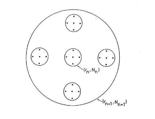
  Figure 2: Reproduction from [2] of a schematic illustration of a deterministic fractal system from where a fractal dimension can be derived. The structure is self-similar, repeating itself at different scales.

  where $\tilde{k}$ and $k$ are constants. By taking the logarithm of equations (1) and (2) and dividing one by the other we get

  $$N_{n}=\sigma{\left(r_{n}\right)}^{D},$$ (3)

  with

  $$\sigma\equiv\frac{N_{0}}{{\left({r_{0}}\right)}^{D}},$$ (4)

  $$D\equiv\frac{\log\tilde{k}}{\log k},$$ (5)

  where $\sigma$ is a prefactor of proportionality related to the lower cutoffs $N_{0}$ and $r_{0}$ of the fractal system, that is, the inner limit where the fractal systems ends, and $D$ is the fractal dimension. If we smooth out the fractal structure we get the continuum limit of equation (3),

  $$N(r)=\sigma r^{D},$$ (6)

  called “generalized mass-length relation” by Pietronero. The de Vaucouleurs density power law is obtained if we now suppose that a portion of the fractal system is contained inside a spherical sample of radius $R_{s}$. Then

  $$\langle\rho\rangle\equiv\frac{N(R_{s})}{V(R_{s})}=\frac{3\sigma}{4\pi}{(R_{s})}^{-\gamma};\ \ \ \gamma\equiv 3-D,$$ (7)

  where $\langle\rho\rangle$ is the average density of the distribution. If we take the value of $\gamma$ as the one found by de Vaucouleurs [19], this implies that the fractal dimension of the distribution is $D\approx 1.3$.

  These are the results of interest for the relativistic approach of this article, and therefore I shall stop here this brief summary of Pietronero’s fractal model. The interested reader can find in [35] a comprehensive account of this fractal approach to cosmology, plus the controversy surrounding the spatial and angular two-point correlation functions and a discussion on multifractals in this context.

  The hierarchical model advanced by Wertz [3] was conceived at a time when fractal ideas had not yet appeared, so in developing his model Wertz was forced to start with a more conceptual discussion in order to offer “a clarification of what is meant by the ‘undefined notions’ which are the basis of any theory” ([3], p. 3). Then he stated that “a cluster consists of an aggregate or gathering of elements into a more or less well-defined group which can be to some extent distinguished from its surroundings by its greater density of elements. A hierarchical structure exists when ith order clusters are themselves elements of an (i+1)th order cluster. Thus, galaxies (zeroth order clusters) are grouped into first order cluster. First order clusters are themselves grouped together to form second order clusters, etc, ad infinitum” (see figure 4).

  Although this sort of discussion may be very well to start with, it demands a precise definition of what one means by a cluster in order to put those ideas on a more solid footing, otherwise the hierarchical structure one is talking

  

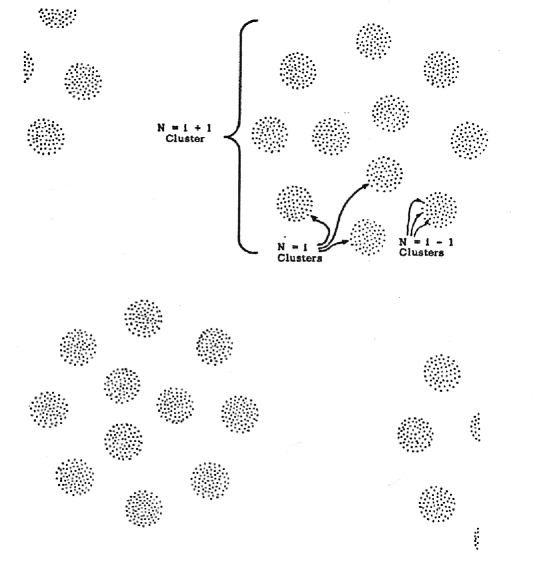
  Figure 4: Reproduction from p. 25 of [3] of a rough sketch cross-section of a portion of an $N=i+2$ cluster of a polka dot model.

  about continues to be a somewhat vague notion. Wertz seemed to have realized this difficulty when later he added that “to say what percentage of galaxies occur in clusters is beyond the abilities of current observations and involves the rather arbitrary judgment of what sort of grouping is to be called a cluster. (…) It should be pointed out that there is not a clear delineation between clusters and superclusters” (p. 8).

  Despite this initially descriptive and somewhat vague discussion about hierarchical structure, which is basically a discussion about scaling in the fractal sense, Wertz did develop some more precise notions when he began to discuss specific models for hierarchy, and his starting point was to assume what he called the “universal density-radius relation”, that is, the de Vaucouleurs density power law, as a fundamental empirical fact to be taken into account in order to develop a hierarchical cosmology. Then if $M(x,r)$ is the total mass within a sphere of radius $r$ centered on the point $x$, he defined the volume density $\rho_{v}$ as being the average over a sphere of a given volume containing $M$. Thus

  $$\rho_{v}(x,r)\equiv\frac{3M(x,r)}{4\pi r^{3}},$$ (8)

  and the global density was defined as being

  $$\rho_{g}\equiv\lim_{r\rightarrow\infty}\rho_{v}(x,r).$$ (9)

  A pure hierarchy is defined as a model universe which meets the following postulates: (i) for any positive value of $r$ in a bounded region, the volume density has a maximum; (ii) the model is composed of only mass points with finite non-zero mean mass; (iii) the zero global density postulate: “for a pure hierarchy the global density exists and is zero everywhere” (see [3] p. 18).

  With this picture in mind, Wertz states that “in any model which involves clustering, there may or may not appear discrete lengths which represent clustering on different scales. If no such scales exist, one would have an indefinite hierarchy in which clusters of every size were equally represented (…). At the other extreme is the discrete hierarchy in which cluster sizes form a discrete spectrum and the elements of one size cluster are all clusters of the next lowest size” (p. 23). Then in order to describe polka dot models, that is, structures in a discrete hierarchy where the elements of a cluster are all of the same mass and are distributed regularly in the sense of crystal lattice points, it becomes necessary for one be able to assign some average properties. So if $N$ is the order of a cluster, $N=i$ is a cluster of arbitrary order (figure 4), and at least in terms of averages a cluster of mass $M_{i}$, diameter $D_{i}$ and composed of $n_{i}$ elements, each of mass $m_{i}$ and diameter $d_{i}$, has a density given by

  $$\rho_{i}=\frac{6M_{i}}{\pi{D_{i}}^{3}}.$$ (10)

  From the definitions of discrete hierarchy it is obvious that

  $$M_{i-1}=n_{i-1}m_{i-1}=m_{i},$$ (11)

  and if the ratio of radii of clusters is

  $$a_{i}\equiv\frac{D_{i}}{d_{i}}=\frac{D_{i}}{D_{i-1}},$$ (12)

  then the dilution factor is defined as

  $$\phi_{i}\equiv\frac{\rho_{i-1}}{\rho_{i}}=\frac{{a_{i}}^{3}}{n_{i}}>1,$$ (13)

  and the thinning rate is given by

  $$\theta_{i}\equiv\frac{\log(\rho_{i-1}/\rho_{i})}{\log(D_{i}/D_{i-1})}=\frac{\log({a_{i}}^{3}/{n_{i}})}{\log a_{i}}.$$ (14)

  A regular polka dot model is defined as the one whose number of elements per cluster $n_{i}$ and the ratio of the radii of successive clusters $a_{i}$ are both constants and independent of $i$, that is, $n$ and $a$ respectively. Consequently, the dilution factor and the thinning rate are both constants in those models,

  $$\phi=\frac{a^{3}}{n},\ \ \ \ \theta=\frac{\log(a^{3}/n)}{\log a}.$$ (15)

  The continuous representation of the regular polka dot model, which amounts essentially to writing the hierarchical model as a continuous distribution, is obtained if we consider $r$, the radius of spheres centered on the origin, as a continuous variable. Then, from equation (12) the radius of the elementary point mass $r_{0}$, is given by

  $$r_{0}=\frac{R_{1}}{a},$$ (16)

  where $R_{N}$ is the radius of a Nth order cluster with $M_{N}$ mass, $V_{N}$ volume, and obviously that $R_{0}=r_{0}$. It follows from equation (16) the relationship between $N$ and $r$,

  $$r=a^{N}r_{0},$$ (17)

  where $R_{N}=r$. Notice that by doing this continuous representation Wertz ended up obtaining an equation (eq. 17) which is nothing more than exactly equation (2) of Pietronero’s single fractal model, although Wertz had reached it by means of a more convoluted reasoning. Actually, the critical assumption which makes his polka dot model essentially the same as Pietronero’s fractal model was to assume the regularity of the model because then $a$ and $n$ become constants. Also notice that this continuous representation amounts to changing from discrete to an indefinite hierarchy, where in the latter the characteristic length scales for clustering are absent. Therefore, in this representation clusters (and voids) extend to all ranges where the hierarchy is defined with their sizes extending to all scales between the inner and possible outer limits of the hierarchy. Hence, in this sense the continuous representation of the regular polka dot model has exactly the same sort of properties as the fractal model discussed by Pietronero.

  From equation (11) we clearly get

  $$M_{N}=n^{N}M_{0},$$ (18)

  which is equal to equation (1), except for a different notation, and hence the de Vaucouleurs density power law is easily obtained as

  $$\rho_{v}=\frac{M_{N}}{V_{N}}=\left[\frac{3M_{0}}{4\pi{r_{0}}^{(\log n/\log a)}}\right]r^{-\theta},$$ (19)

  where $\theta$ is the thinning rate

  $$\theta=3-\left(\frac{\log n}{\log a}\right).$$ (20)

  Notice that equations (19) and (20) are exactly equations (7), where $\gamma$ is now called the thinning rate. Finally, the differential density, called conditional density by Pietronero, is defined as

  $$\rho_{d}\equiv\frac{1}{4\pi r^{2}}\frac{dM(r)}{dr}=\left(1-\frac{\theta}{3}\right)\rho_{v}.$$ (21)

  From the presentation above it is then clear that from a geometrical viewpoint Wertz’s continuous representation of the regular polka dot model is nothing more than Pietronero’s single fractal model. However, the two approaches may be distinguished from each other by some important conceptual differences. Basically, as Pietronero clearly defines the exponent of equation (3) as a fractal dimension, that immediately links his model to the theory of critical phenomena in physics, and also to nonlinear dynamical systems, bringing a completely new perspective to the study of the distribution of galaxies, with potentially new mathematical concepts and analytical tools to analyze this problem. In addition, it also strongly emphasizes the fundamental importance of scaling behaviour in the observed distribution of galaxies and the exponent of the power law, as well as pointing out the appropriate mathematical tool to describe this distribution, namely the fractal dimension. All that is missing in Wertz’s approach, and his thinning rate is just another parameter in his description of hierarchy, without any special physical meaning attached to it. Therefore, in this sense his contribution started and remained as an isolated work, forgotten by most, and which could even be viewed simply as an ingenious way of modelling Charlier’s hierarchy, but nothing more.

  Nonetheless, it should be said that this discussion must not be viewed as a critique of Wertz’s work, but simply as a realization of the fact that at Wertz’s time nonlinear dynamics and fractal geometry were not as developed as at Pietronero’s time, if developed at all, and therefore Wertz could not have benefited from those ideas. Despite this it is interesting to note that with less data and mathematical concepts he was nevertheless able to go fairly far in discussing scaling behaviour in the distribution of galaxies, developing a model to describe it in the context of Newtonian cosmology, and even suggesting some possible ways of investigating relativistic hierarchical cosmology.

  4 A RELATIVISTIC APPROACH TO HIERARCHICAL (FRACTAL) COSMOLOGY

  In this section I shall start to develop a relativistic cosmology based on the ideas expressed by Pietronero and Wertz and discussed in the previous section. The notation used will be the same as in Pietronero’s approach with minor changes, but some quantities will be referred by the names used by Wertz.

  The first thing necessary for one to start a relativistic model is obviously the choice of the appropriate metric for the problem under consideration. In the case of a relativistic fractal cosmology, we need an inhomogeneous metric so that it becomes possible to derive a relativistic version of Pietronero’s relation (6). [Note added in 2009– Regarding this point, a different perspective is advanced in Refs. [51, 52, 53] where fractals can be accommodated within a spatially homogeneous metric.] Following the simple geometrical ideas outlined by both Wertz and Pietronero, spherical symmetry seems to be reasonable enough to start with. By means of a similar reasoning, a dust distribution of matter also seems reasonable enough to start with, and in that way we have outlined some requirements which are equivalent to making some strong simplifications that seem enough for a simple exploratory relativistic fractal cosmological model. Bearing this discussion in mind, the Tolman solution suggests itself as it is the general solution of the Einstein’s field equations for spherically symmetric dust in comoving coordinates [40]. However, the Tolman solution is spherically symmetric about one point, and constructing a cosmological model with it means that we would be giving up the Copernican principle which states that there are no preferred points in the universe. Despite this difficulty, if we assume that there could be an upper cutoff to homogeneity in our fractal system, we can construct a model using a variation of the Einstein-Straus geometry, also known as “Swiss-cheese” models, with an interior solution provided by the Tolman metric surrounded by a Friedmann spacetime. Such a model needs to solve the junction conditions between the two metrics in order to achieve a smooth transition, and the solution imposes strong restrictions to the mass inside the Tolman region, namely that the gravitational mass inside must be the same as if the whole spacetime were Friedmannian and the Tolman region were never there [41]. By means of such scheme we are able to satisfy the Copernican principle in our relativistic fractal model, but for reasons that will become clear later, such geometry is not really mandatory. 

  In order to make use of Tolman’s models as descriptors of observations, it is necessary first of all to derive the observational relations in this metric. I shall present next a brief summary of the Tolman spacetime followed by its observational relations, but without demonstration. Full details about the observational relations in this metric can be found in [41].

  The Tolman metric with $\Lambda=0$ and $c=G=1$ may be written as

  $$dS^{2}=dt^{2}-\frac{{R^{\prime}}^{2}}{f^{2}}dr^{2}-R^{2}d\Omega^{2};\ \ \ r\geq 0,\ \ \ R(r,t)>0,$$ (22)

  where

  $$d\Omega^{2}=d\theta^{2}+\sin^{2}\theta d\phi^{2},$$

  and $f(r)$ is an arbitrary function. The Einstein’s field equations for the metric (22) reduces to a single equation,

  $$2R{\dot{R}}^{2}+2R(1-f^{2})=F,$$ (23)

  where $F(r)$ is another arbitrary function. The proper density is given by

  $$8\pi\rho=\frac{F^{\prime}}{2R^{\prime}R^{2}},$$ (24)

  and the dot means $\partial/\partial t$ and the prime $\partial/\partial r$.

  The solution of equation (23) has three distinct cases according as $f^{2}=1$, $f^{2}>1$ and $f^{2}<1$, these cases being termed, respectively, parabolic, hyperbolic and elliptic Tolman models. In the parabolic models ($f^{2}=1$) the solution of equation (23) is

  $$R=\frac{1}{2}{(9F)}^{1/3}{(t+\beta)}^{2/3},$$ (25)

  where $\beta(r)$ is a third arbitrary function.  In the hyperbolic models ($f^{2}>1$) the solution of equation (23) may be written in terms of a parameter $\Theta$

  $$R=\frac{F(\cosh 2\Theta-1)}{4(f^{2}-1)},$$ (26)

  $$t+\beta=\frac{F(\sinh 2\Theta-2\Theta)}{4{(f^{2}-1)}^{3/2}},$$ (27)

  and finally in the elliptic models ($f^{2}<1$) the solution of equation (23) may be written as

  $$R=\frac{F(1-\cos 2\Theta)}{4\mid f^{2}-1\mid},$$ (28)

  where

  $$t+\beta=\frac{F(2\Theta-\sin 2\Theta)}{4{\mid f^{2}-1\mid}^{3/2}}.$$ (29)

  The three classes of the Tolman solution are the equivalent of flat, open and closed Friedmann models.

  The observational relations in Tolman’s spacetime necessary in this work have been calculated in [41], and I shall only state here the results obtained. The luminosity distance in the Tolman model is given by

  $$d_{\ell}=R{(1+z)}^{2}.$$ (30)

  The redshift may be written as

  $$1+z={(1-I)}^{-1},$$ (31)

  where the function $I(r)$ is the solution of the differential equation 

  $$\frac{dI}{dr}=\frac{{\dot{R}}^{\prime}}{f}(1-I).$$ (32)

  The number of sources which lie at radial coordinate distances less than $r$ as seen by the observer at $r=0$ and along the past light cone, that is, the cumulative number count, is given by

  $$N_{c}(r)=\frac{1}{4M_{G}}\int\frac{F^{\prime}}{f}dr,$$ (33)

  where $M_{G}$ is the average galactic rest mass ( $\sim 10^{11}M_{\odot}$). The volume $V$ of the sphere which contains the sources, and the volume (average) density $\rho_{v}$, have the form

  $$V(r)\equiv\frac{4}{3}\pi{(d_{\ell})}^{3}=\frac{4}{3}\pi R^{3}{(1+z)}^{6},$$ (34)

  $$\rho_{v}\equiv\frac{N_{c}(r)M_{G}}{V(r)}=\frac{3}{16\pi R^{3}{(1+z)}^{6}}\int\frac{F^{\prime}}{f}dr.$$ (35)

  The relativistic version of Pietronero’s generalized mass-length relation used in this work is given by

  $$N_{c}=\sigma{(d_{\ell})}^{D},$$ (36)

  and if we substitute equations (34) and (36) into equation (35) we get a relativistic version of the de Vaucouleurs density power law

  $$\rho_{v}=\frac{3\sigma M_{G}}{4\pi}{(d_{\ell})}^{-\gamma},$$ (37)

  where

  $$\gamma=3-D$$ (38)

  is Wertz’s thinning rate. Equation (37) gives the volume density for an observed sphere of certain radius $d_{\ell}$ that contains a portion of the fractal system. All observational relations above must be calculated along the past light cone, so if we adopt the radius coordinate $r$ as the parameter along the backward null cone, we can then write the radial null geodesic of metric (22) as

  $$\frac{dt}{dr}=-\frac{R^{\prime}}{f}.$$ (39)

  Notice that along the past light cone $R=R[r,t(r)]$, where $t(r)$ is the solution of equation (39), and this is the function to be used in the relations above such that they are really calculated along the null geodesic.

  The next step in order to find fractal solutions in the Tolman model is to take advantage of its own freedom, given by the arbitrariness of the functions $f(r)$, $F(r)$ and $\beta(r)$, such that we are able to simulate the desired distribution of dust by means of a method similar to the one employed by Bonnor [28], but in a more complex and realistic context than his. However, in order to do so we have to solve the past radial null geodesic (39) and then the equation for the redshift (32), an almost impossible task to be carried out analytically due to the fact that the functions $R$, $R^{\prime}$, ${\dot{R}}^{\prime}$ form complex algebraic expressions [41], and so a numerical solution becomes inevitable. Such an approach can be essentially described as follows.

  For a fractal structure as described above, the de Vaucouleurs density power law holds. Hence equation (37) may be written as

  $$\log\rho_{v}=a_{1}+a_{2}\log d_{\ell},$$ (40)

  where $a_{1}$ and $a_{2}$ are constants related to the lower cutoff of the fractal pattern and its fractal dimension,

  $$D=a_{2}+3,$$ (41)

  $$\sigma=\frac{4\pi}{3M_{G}}\mbox{exp}(a_{1}).$$ (42)

  Generally speaking, the numerical algorithm for finding those fractal solutions can be summarized as follows:

  1. start by choosing $f(r)$, $F(r)$, $\beta(r)$;

  2. solve numerically the two ordinary differential equations (32) and (39);

  3. evaluate the observational relations along the past light cone: $d_{\ell}$, $\rho_{v}$, $N_{c}$, $z$, $V$;

  4. fit a straight line with the points obtained by numerical integration, according to equation (40);

  5. is the fitting linear and with negative slope?

  6. if the answer is no, then choose other functions $f(r)$, $F(r)$, $\beta(r)$ and go all over again; else stop: a fractal solution was modelled and $D$ and $\sigma$ are easily found.

  The description above is very schematic since many other important details like root finding algorithm for equations (27) and (29), initial conditions for the ode’s, numerical integrator, etc, have to be considered. A full discussion of the numerical problems involved in this method can be found in [41, 42]. In any case, from the description above it is obvious that if the distribution of dust remains homogeneous throughout the past null geodesic, the volume density will not change and $\log\rho_{v}=\mbox{constant}$, and $D=3$. In this case the plot $\log\rho_{v}$ vs. $\log d_{\ell}$ will be a straight line with zero slope.

  Before closing this section, a few words are necessary here in order to explain why the luminosity distance $d_{\ell}$ was chosen as the measurement of distance in this relativistic approach to fractal cosmology. As is well known, in relativistic cosmology we do not have an unique way of measuring the distance between source and observer since their separation depends on circumstances. We can, for instance, make use of geometrically defined distances like the proper radius, or observationally defined distances like the luminosity distance or the observer area distance (also known as angular diameter distance) in order to say that a certain object lies at a certain distance from us. The circumstances which tell us which definition to use can also be determined on observational grounds, and so if we only have at our disposal the apparent magnitudes of galaxies we associate to each of them the luminosity distance and use such measurement in our analysis. On the other hand, if these apparent magnitudes are corrected by the redshift of the sources, we can then associate the corrected luminosity distance, which is the same as the observer area distance obtained if we have the apparent size of the objects [43], and, therefore, another kind of distance measure is obtained. Any of these observational distances are as valid as any other, as real as any other, with the choice being dictated by the availability of data, the nature of the problem being treated and its convenience, but they will only have the same value at $z\ll 1$, varying sometimes widely for larger $z$ (see [44] for a comparison of these distances in simple cosmological models). In this work we are interested in observables because we seek to compare theory with observations, and this means that geometrical distances are of no interest here. Consequently, the approach of this relativistic cosmological model is different from others where unobservable coordinate distances (differences between coordinates) and separations (integration of the line element $dS$ over some previously defined surface) are taken as measure of distance, and in order to develop a treatment coherent with the observational approach of this problem we need to make a choice among the observational distances based on the nature of the problem and the observations available. It is the intention of this work to propose a relativistic extension of Pietronero-Wertz model in order to describe the observed scaling behaviour of the distribution of galaxies detected by the recent all-sky redshift surveys, and in this area of research it is usual for observers to take the luminosity distance as their indicator of distance (for example, [45] does use $d_{\ell}$ in its statistical analysis of a sample of iras galaxies). It seems therefore perfectly reasonable to take the luminosity distance as the most appropriate definition of distance to use in the context of this work, because what is sought is to mimic the current methodology followed by many observers in this field, and to carry out a comparison between the theoretical predictions of this relativistic cosmological model and the observational results brought by the redshift surveys.

  5 HOW INHOMOGENEOUS IS A “HOMOGENEOUS” UNIVERSE?

  The observational relations presented in the previous section were derived with the clear intention of developing a relativistic fractal model in the sense of Pietronero and Wertz, but as we shall see in this section, the application of these same observational relations to the spatially homogeneous Friedmann spacetime bring to light some very interesting and unexpected results. [Note added in 2009– See Refs. [50, 51, 52, 53, 55, 56, 57] for further developments of these ideas and more in depth discussions on the results below.]

  In order to see how those results are achieved, let me say first of all that the question which motivated the application of the observational relations above to the Friedmann spacetime came from the realization that fractal dimensions, in the sense of Pietronero and Wertz, were defined in Euclidean spaces, and it is not clear beforehand whether equation (36) will give the value $D=3$ for the fractal dimension in the Friedmann metric when we are dealing with observables. One can see more clearly this point if we remember that this metric is spatially homogeneous, that is, it has constant local densities at constant time coordinates, and when we integrate along the past light cone, going through hypersurfaces of $t$ constant with each one having different values for the proper density, one may argue that $D$ could depart from the value 3 even in a spatially homogeneous spacetime [41]. With this point in mind, we may go even further and ask whether or not even the Friedmann metric could be compatible with a fractal description of cosmology [46], even in the strongly simplified relativistic version of Pietronero-Wertz model presented here. In order to try to answer those questions, it is convenient to start with the analytically feasible Einstein-de Sitter model.

  It is shown in the appendix that the Einstein-de Sitter model can be obtained from Tolman’s spacetime as a special case when

  $$f(r)=1,\ \ \ F(r)=\frac{8}{9}r^{3},\ \ \ \beta(r)=\beta_{0},$$ (43)

  where $\beta_{0}$ is a constant. In this case the two differential equations (32) and (39) are easily integrated from $I=t=r=0$ to $I(r)$ and $t(r)$, respectively yielding

  $$1-I={\left(\frac{3{\beta_{0}}^{1/3}-r}{3{\beta_{0}}^{1/3}}\right)}^{2},$$ (44)

  $$3{(t+\beta_{0})}^{1/3}=3{\beta_{0}}^{1/3}-r.$$ (45)

  Therefore, along the past light cone the solution (25) of the field equation and its derivatives take the form

  $$R=\frac{r}{9}{(3{\beta_{0}}^{1/3}-r)}^{2};\ \ \ R^{\prime}=\frac{1}{9}{(3{\beta_{0}}^{1/3}-r)}^{2};\ \ \ {\dot{R}}^{\prime}=2{(3{\beta_{0}}^{1/3}-r)}^{-1}.\ \ \$$ (46)

  With the results above, we can easily obtain the observational relations in the Einstein-de Sitter model. The redshift, luminosity distance, cumulative number count, observed volume, volume and local densities are respectively given by

  $$1+z={\left(\frac{3{\beta_{0}}^{1/3}}{3{\beta_{0}}^{1/3}-r}\right)}^{2},$$ (47)

  $$d_{\ell}=\frac{9r{\beta_{0}}^{4/3}}{{(3{\beta_{0}}^{1/3}-r)}^{2}},$$ (48)

  $$N_{c}=\frac{2r^{3}}{9M_{G}},$$ (49)

  $$V=\frac{12\pi r^{3}{(3\beta_{0})}^{4}}{{(3{\beta_{0}}^{1/3}-r)}^{6}},$$ (50)

  $$\rho_{v}=\frac{{(3{\beta_{0}}^{1/3}-r)}^{6}}{54\pi{(3\beta_{0})}^{4}},$$ (51)

  $$\rho=\frac{1}{6\pi}{\left(\frac{3}{3{\beta_{0}}^{1/3}-r}\right)}^{6}.$$ (52)

  We can see that the local and volume densities change along the past null geodesic, and this is obvious from the dependence on $r$ in both equations (51) and (52). That happens because along the past light cone the integration goes through different surfaces of $t$ constant, and in this sense the Einstein-de Sitter model does appear to be inhomogeneous along the backward null cone. The presence of the coordinate $r$ in equation (52) does not mean a spatially inhomogeneous local density, since $r$ is only a parameter along the past null geodesic, and due to equation (45) each value of $r$ corresponds to a single value of $t$, that is, each $r$ corresponds to a specific $t=$constant hypersurface given by equation (45). However, as along the null geodesic the local density effectively changes as it goes through different surfaces of constant time coordinate, hence in this sense the model can be thought of as inhomogeneous. The volume density may also change inasmuch as it is being measured through these same hypersurfaces of $t$ constant, where each one has different values for the proper density, and being a cumulative density, $\rho_{v}$ averages at bigger and bigger volumes in a way that adds more and more different local densities of each spatial section of the model.

  Another interesting result follows if we look at the asymptotic limit of the equations above. As the function $\beta(r)$ determines the local time at which $R=0$ (see the appendix), the surface $t+\beta=0$ is a surface of singularity, which means that the physical region considered is given by the condition $t+\beta>0$. Considering equation (45), it is obvious that $r=3{\beta_{0}}^{1/3}$ corresponds to the surface of singularity, meaning that the physical region of the model is given by the condition $0\leq r\leq 3{\beta_{0}}^{1/3}$. Therefore, when $r\rightarrow 3{\beta_{0}}^{1/3}$ the observational relations breakdown since $z\rightarrow\infty$, $V\rightarrow\infty$, $d_{\ell}\rightarrow\infty$, $\rho\rightarrow\infty$ and $\rho_{v}\rightarrow 0$.

  So we can see that the volume density vanishes asymptotically when observables are plotted, and this result is a consequence of the definition adopted here for the volume density since at the big bang singularity hypersurface the observed volume is infinity, but the total mass is finite. Thus we may say that the following limit holds in the Einstein-de Sitter cosmology:

  $$\lim_{d_{\ell}\rightarrow\infty}\rho_{v}=0.$$ (53)

  Comparing with equation (9), this result means that this relativistic cosmology obeys the zero global density postulate for a pure hierarchy, as defined by Wertz (and conjectured later by Pietronero), and therefore, we may that under the appropriate definitions the Einstein-de Sitter model seems to meet all postulates of a pure hierarchical model, in the sense of Wertz.

  The zero global density postulate was formulated by Wertz since it is a logical result if one takes the Newtonian version of the de Vaucouleurs density power law to its logical asymptotic limit. However, this result has been repeatedly used as a fundamental reason why the universe cannot be hierarchical (or fractal) at larger scales because this postulate not only supposedly contradicts the spatially homogeneous Friedmann model [37], thought to be the correct cosmological model, but also is considered conceptually unacceptable. For instance, [27] states that “if the universe is really the Friedmann type on large scale (…) the inhomogeneous structure must cease on large enough scale”. It is then clear from equation (53) that this is may be a rather misleading approach to relativistic fractal cosmology, and even to cosmology in general, since we definitively can have an observationally based interpretation of the Friedmann model where it has no well defined average density, and is inhomogeneous, with asymptotically zero global density along the past light cone. Therefore, it seems to be an inescapable conclusion that having or not having zero global density in the model is just a question of interpretation. 

  The inhomogeneity of the Einstein-de Sitter model can be graphically seen in figure 6 where the volume density is plotted against the luminosity distance. At close ranges the model is homogeneous, with the average showing no significant departure from a constant value. This means that at very close ranges the volume density is being measured at our constant time hypersurface, but once the scale increases the average starts to change, which means that $\rho_{v}$ begins to be calculated at regions where the local density differs from the value at our “now” ($t=0$). In other words, once the volume density starts to change significantly we would have a significant distancing from the initial time hypersurface, going towards earlier epochs of the model. The plot then shows, in a quantitative way, the scale where theoretically the Einstein-de Sitter model no longer is observationally homogeneous, which in the case of the plot of figure 6 is at about $z\approx 0.04$, or $d_{\ell}\approx 160$ Mpc. It is easy to show that a 30% decrease in $\rho_{v}$ from the value at $t=0$ (now) happens at about $z\approx 0.1$, or $d_{\ell}\approx 500$ Mpc, and therefore, this is approximately the maximum range up to where the homogeneity of the Einstein-de Sitter model can be observed. In other words, as this limit is obtained by solving the past null

  

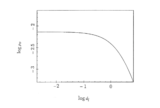
  Figure 6: Plot of $\rho_{v}$ vs. $d_{\ell}$ in the Einstein-de Sitter model for the range $0.001\leq r\leq 1.5$ and with $\beta_{0}=2.7$ (distance is given in Gpc, and $H_{0}=75\ \mbox{km}\ {\mbox{s}}^{-1}\ {\mbox{Mpc}}^{-1}$ is assumed). The distribution does not appear to remain homogeneous along the null geodesic and the fractal dimension departs from the initial value 3 [46].

  geodesic equation and using the result in observational relations, we have here a clear evidence that relativistic effects become important in cosmology at very close ranges, and this offers us an observationally based methodology that in principle allows us to ascertain quantitatively such ranges in different scenarios.

  Another interesting aspect that comes out of the analysis of figure 6 is the fact that the fractal dimension of the distribution has only the value $D=3$ in the homogeneous, or flat region of the plot. Beyond this it starts to decrease, effectively making the thinning rate in equation (37) a function of position which, in other words, is incompatible with a single fractal description for the distribution of dust in the Einstein-de Sitter cosmology.

  The open and recollapsing Friedmann models also behave in a similar inhomogeneous manner as compared to the Einstein-de Sitter model, although the ranges where the departure from homogeneity starts are different. Figure 8 shows the numerical solution for the observational

  

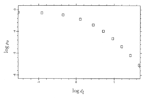
  Figure 8: Numerical results for $\rho_{v}$ vs. $d_{\ell}$ in the open Friedmann model model for the range $0.001\leq r\leq 1.5$ and with $\beta_{0}=3.6$ and $\Omega_{0}\approx 0.2$. The deviation from a homogeneous initial region is also visible, and starts at about $d_{\ell}\approx 250$ Mpc [42].

  

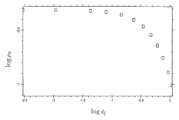
  Figure 10: Numerical results for $\rho_{v}$ vs. $d_{\ell}$ in the recollapsing Friedmann model model for the range $0.001\leq r\leq 1.5$ and with $\beta_{0}=0.7$ and $\Omega_{0}\approx 4$. The departure from the homogeneous initial region starts at very close range, at about $d_{\ell}\approx 30$ Mpc [42].

  relations in the $K=-1$ Friedmann model, and figure 10 shows the same plot for the recollapsing model [42]. We can clearly see the deviation from homogeneity in both models, although the former starts to deviate at about $d_{\ell}\approx 250$ Mpc while in the latter that happens at $d_{\ell}\approx 30$ Mpc. Due to the similarity of the graphs, it seems reasonable to conclude that all Friedmann models appear to obey Wertz’s zero global density postulate.

  6 TOLMAN FRACTAL SOLUTIONS

  Once the observational relations and the numerical methodology for finding fractal solutions in the Tolman model is developed, we can go to the stage of actually specializing the free functions of Tolman’s metric in order to see which ones, if any, do have fractal behaviour.  Nonetheless, some criteria must be met by those solutions such that some essential observational constraints are obeyed. Those criteria for choosing and accepting the solutions can be listed as follows:

  • linearity of the redshift-distance relation for $z<1$;

  • the Hubble constant within the currently accepted range $40\ \mbox{km}\ {\mbox{s}}^{-1}\ {\mbox{Mpc}}^{-1}<H_{0}<100\ \mbox{km}\ {\mbox{s}}^{-1}\ {\mbox{Mpc}}^{-1}$;

  • constraint in the fractal dimension of $1<D<2$;

  • obedience to the Vaucouleurs’ density power law $\rho_{v}\propto{d_{\ell}}^{-\gamma}$.

  By means of the methodology described in section 4, a systematic search for fractal solutions was carried out [42], but only hyperbolic type solutions were found to meet all the criteria outlined above. Here I shall only show the simplest hyperbolic fractal solution obtained, since the other classes of fractal solutions did not meet all criteria above. A complete discussion and presentation of the other solutions can be found in [42].

  The particular form of the three functions that led to fractal behaviour in hyperbolic models is as follows:

  $$\left\{\begin{array}[]{ll}f=\cosh r,\\ F=\alpha r^{p},\\ \beta=\beta_{0},\end{array}\right.$$ (54)

  where $\alpha$, $p$, and $\beta_{0}$ are positive constants. The experience with the numerical simulations show that $\alpha$ must be around $10^{-4}$ to $10^{-5}$ and $p$ and $\beta_{0}$ can vary from around 0.5 to 4. Figure 12 shows the power law behaviour of $\rho_{v}$ vs. $d_{\ell}$ of the model formed by functions (54), with a fractal dimension of $D=1.4$. The straight line fitted according to equation (40) is also clearly visible. Figure 14 is the redshift-distance diagram of the same model where we can see the good linear approximation given by functions (54). The slope of the points gives $H_{0}\cong 80\ \mbox{km}\ {\mbox{s}}^{-1}\ {\mbox{Mpc}}^{-1}$, and it is interesting to note that recent measurements made by two different methods suggest a Hubble constant very close to this value [48]. Actually, for $\beta_{0}=3.6$, the value used to get the results shown in figures 12 and 14, we would have an age of the universe of about 12 Gyr, which is a lower limit if we consider the age of globular clusters [48]. Therefore, also in this point of the age of the universe, the model (54) agrees reasonably well with observations. The integrations with functions (54) were stopped at $z\cong 0.07$, which corresponds to the luminosity distance $d_{\ell}\cong 270$ Mpc and this is the redshift depth of the iras redshift survey [9]. Finally, figure 16 shows the results for cumulative number counting vs. redshift produced by the model under consideration.

  

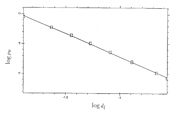
  Figure 12: Results of the volume density $\rho_{v}$ vs. luminosity distance $d_{l}$ of the hyperbolic model (54). The integration is in the interval $0\leq r\leq 0.07$ and the constants are $\alpha=10^{-4},\ p=1.4,\ \beta_{0}=3.6$. The fitting coefficients calculated are $a_{1}=-6.0$ and $a_{2}=-1.6$, giving a fractal dimension $D=1.4$ and a lower cutoff constant $\sigma=8.7\times 10^{5}$.

  

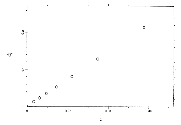
  Figure 14: Distance-redshift diagram obtained with the hyperbolic model of functions (54). The slope of the diagram obtained for $d_{\ell}$ vs. $z$ gives $H_{0}\cong 80\ \mbox{km}\ {\mbox{s}}^{-1}\ {\mbox{Mpc}}^{-1}$, a value which is within the current uncertainty in the Hubble constant.

  

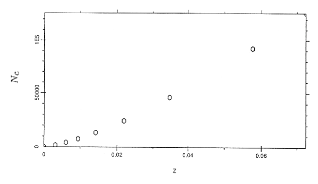
  Figure 16: Plot of the results for the cumulative number counting $N_{c}$ vs. the redshift $z$ given by the integration of the model (54) with the same parameters as in figure 12.

  As mentioned above, there are strict limits on the values of the parameters $\alpha$, $p$ and $\beta_{0}$, and by means of numerical experimentation it was found that outside the ranges stated above, the fractality of the model (54) is destroyed. Therefore, it seems that this fractal model is structurally fragile as a variation of the parameters of the model can produce a qualitative change in its behaviour.

  As closing remarks, it can be shown [42] that the model (54) remains fractal at different epochs, with a remarkable constancy in the fractal dimension. In addition, if a Friedmann metric is joined to the solution (54), we can use the internal Tolman solution to find the Friedmann model which best fits another cosmological model that gives a realistic representation of the universe (in this case, the Tolman model given by equations [54]), including all inhomogeneities down to some specified length scale mandatory. By doing this procedure, it can be shown [42] that the best Friedmann model is an open one, with $H_{0}=83\ \mbox{km}\ {\mbox{s}}^{-1}\ {\mbox{Mpc}}^{-1}$ and $\Omega_{0}\cong 0.002$. This low value for $\Omega_{0}$ is explained as due to the fact that in this approach no kind of dark matter was considered, but only the luminous matter associated with the galaxies, which are assumed to form a fractal system. Galactic luminous matter gives a value for $\Omega_{0}$ of the same order of magnitude as the one found above.

  Joining an external Friedmann metric to the internal inhomogeneous solution was initially thought to be a good way of modelling a possible crossover to homogeneity to the fractal system. However, as the Friedmann metric looks inhomogeneous at larger scales when measured along the past light cone, this result seems to imply that this external solution is not really mandatory.

  7 CONCLUSIONS AND DISCUSSION

  This work presented in essence a different approach for modelling the large scale distribution of galaxies, whose main idea is to assume the non-orthodox, but old principle that the empirically observed self-similarity of this distribution is a fundamental fact to be taken into account in any model that attempts a realistic representation of the distribution of galaxies. Under this philosophy, a simple relativistic model was advanced, model which is essentially a translation to a relativistic framework of the Newtonian hierarchical (fractal) cosmology developed by Wertz and Pietronero. This is a simple exploratory model, which although it had to assume some strong simplifications, it is able to obtain some interesting new results, like the inhomogeneity of the Friedmann model, once the observational relations derived for this fractal model are used in this metric. It also shows that the idea of a vanishing global density, postulated for hierarchical (fractal) cosmologies, is not necessarily in contradiction with currently accepted cosmological models like the Einstein-de Sitter one, being essentially a question of using the appropriate definitions for density and distance. A general methodology for searching fractal solutions is also advanced, and this methodology is able to successfully find them, showing that solutions of Einstein’s field equations approximating a single fractal structure do exist.

  In addition to those points, some remarks about the method and the solution should be made. In the first place, the best numerical simulation presented an open, ever expanding model for the large scale distribution of galaxies, and although such class of models are obviously favoured by the simulations, it must be said that flat or recollapsing models are not at all ruled out as there may be some more complex forms for the functions $f(r)$, $F(r)$ and $\beta(r)$ which produce observationally compatible models, but which were not investigated. Secondly, in view of the results obtained with the fractal inspired observational relations, it seems that observable average densities appear to be physically interesting for the characterization of cosmological models. In particular they are important in the description of a fractal system, and in the determination of the limits of validity of the homogeneous hypothesis. Thirdly, as discussed in the Introduction, the model showed here provides a description for the possible fractal structure of the universe, but as in the problem of coastlines, it does not provide an answer to the question of where this fractal system came from, its origins, and why the large scale luminous matter appears to follow a fractal pattern.

  To try to answer this last point, it may be crucial a deeper study of the dynamics of the field equations, or even the particular model showed here, as their nonlinearity may provide some important clues such that one may be able to get closer to answering the question of where this fractal pattern came from. In this respect there are some aspects that may possibly help in this direction. In the first place, structural fragility seems to be a reality in the fractal model discussed (and the others presented in [42]), since there is evidence for this behaviour from the numerical experimentations themselves. Secondly, from the theory of dynamical systems we know that strange attractors have a fractal pattern in phase space. Therefore, the obvious questions is when we see, along the past null geodesic, a self-similar fractal pattern, could that mean that a strange attractor is lurking from behind the scenes? In this case, how can we characterize it? In addition to this, as in some chaotic dynamical systems, could there exists a possible link between the fractal dimension and the Lyapunov exponents in this cosmological context?

  Those questions are already in the realm of the second stage of the physicist’s approach to dynamical systems, as discussed in the Introduction, and by their own nature, answering them will probably be a very challenging task. In any case, a complete or partial response to any of these points is likely to shed some light on the underlying dynamics of the relativistic field equations in this specific model or, perhaps, in more general ones.

  ACKNOWLEDGMENTS

  Thanks go to the organizing committee for this interesting and informative workshop, and in special to David Hobill for the smooth way the local organization was carried out.

  APPENDIX. The Friedmann metric as a special case of the Tolman solution

  The aim of this appendix is to show how the Tolman solution can be reduced to the Friedmann metric by means of the specializations of the functions $f(r)$, $F(r)$, $\beta(r)$, and the physical differences between the two metrics. This may be useful for those not familiar with the Tolman solution.

  It can be shown, by calculating the junction conditions between the Tolman and Friedmann metrics [41], that in order to obtain the latter from the former we have to assume that

  $$R(r,t)=a(t)\ g(r),\ \ \ \ f(r)=g^{\prime}(r).$$ (55)

  By substituting equations (55) into the metric (22) we get

  $$dS^{2}=dt^{2}-a^{2}(t)\left\{dr^{2}+g^{2}(r)\left[d\theta^{2}+\sin^{2}\theta d\phi^{2}\right]\right\},$$ (56)

  which is a Friedmann metric if

  $$g(r)=\left\{\begin{array}[]{ll}\sin r,&\\ r,&\\ \sinh r.&\end{array}\right.$$ (57)

  If we now substitute equations (55) in equation (24) and integrate it, that gives

  $$\frac{F}{4}=\frac{4\pi}{3}\rho a^{3}g^{3}.$$ (58)

  It is worth noting that the time derivative of the equation above gives the well-known relation for the matter-dominated era of a Friedmann universe:

  $$\frac{d}{dt}\left(\rho a^{3}\right)=0.$$

  Equation (58) is necessary in order to deduce the usual Friedmann equation. This is possible by substituting equations (55) and (58) into equation (23). The result may be written as

  $$\dot{a}^{2}=\frac{8\pi}{3}\rho a^{2}-K$$ (59)

  where

  $$K=\frac{1-{g^{\prime}}^{2}}{g^{2}}.$$

  It is easy to see that $K=+1,\ 0,\ -1$ if $g=\sin r,\ r,\ \sinh r$, respectively, and this shows that equation (59) is indeed the usual Friedmann equation. Let us now write equation (59) in the form

  $$\frac{\dot{a}^{2}g^{2}}{2}-\frac{m}{ag}=-\left(1-{g^{\prime}}^{2}\right)$$ (60)

  where

  $$m(r)=\frac{4\pi}{3}\rho a^{3}g^{3}.$$ (61)

  Equation (60) is interpreted as an energy equation [49] and, in consequence, $m(r)$ is the gravitational mass inside the coordinate $r$. Thus $4m(r)=F(r)$ and this shows the role of the function $F(r)$ in providing the gravitational mass of the system. In addition, equation (60) shows that the function $f(r)$ in Tolman’s spacetime gives the total energy of the system.

  The function $\beta(r)$ gives the big bang time of the model, and this can be seen as follows. If “now” is defined as $t=0$ and if $\beta(r)=0$, then the hypersurface $t=0$ is singular, that is, $R=0$ everywhere . So $\beta(r)$ gives the age of the universe which in Tolman’s spacetime may change if different observers are situated at different radial coordinates $r$. This is a remarkable departure from Friedmann’s model that gives the same age of the universe for all observers on a hypersurface of constant $t$. In other words, in a Friedmann universe the big bang is simultaneous while in a Tolman one it may be non-simultaneous, that is, the big bang may have occurred at different proper times in different locations. As a consequence another essential ingredient in reducing the Tolman metric to Friedmann is $\beta=$ constant, and so the linkage between $\beta$ and the Hubble constant is of the form

  $$\frac{\dot{R}}{R}=\frac{\dot{a}}{a}=H(t),\ \ \ \mbox{for}\ \ \beta=\beta_{0},$$ (62)

  where $\beta_{0}$ is a constant. Considering equation (25) it is straightforward to conclude that

  $$\beta_{0}=\frac{2}{3H_{0}},$$ (63)

  where $H_{0}=H(0)$. Equation (63) gives the relationship between $\beta_{0}$ and the Hubble constant $H_{0}$ in a Einstein-de Sitter universe.

  Bearing this discussion in mind it is easy to see that the usual Friedmann universe requires that $g=\sin r$, $r$, $\sinh r$ and $F=b_{1}\sin^{3}r$, $\frac{8}{9}r^{3}$, $b_{2}\sinh^{3}r$, which are respectively the cases for $K=+1$, $0$, $-1$. The positive constants $b_{1}$ and $b_{2}$ are scaling factors necessary to make the density parameter $\Omega$ equal to any value different from one in the open and closed models.

  Let us now extend equation (63) to the $K=\pm 1$ Friedmann cases. Considering the specializations above, that permit us to get the Friedmann metric from the Tolman solution, and assuming $t=0$ as our “now”, that is, $t=0$ being the time coordinate label for the present epoch, it is straightforward to show that the present value $H_{0}$ for the Hubble constant in the closed Friedmann model is given by

  $$H_{0}=\frac{4\sin 2\Theta_{0}}{b_{1}{(1-\cos 2\Theta_{0})}^{2}},$$ (64)

  where $\Theta_{0}$ is the solution of

  $$4\beta_{0}=b_{1}(2\Theta_{0}-\sin 2\Theta_{0}),$$ (65)

  and $\beta(r)=\beta_{0}$ is a constant that gives the age of the universe. In the open Friedmann case we will have then

  $$H_{0}=\frac{4\sinh 2\Theta_{0}}{b_{2}{(\cosh 2\Theta_{0}-1)}^{2}},$$ (66)

  and

  $$4\beta_{0}=b_{2}(\sinh 2\Theta_{0}-2\Theta_{0}).$$ (67)

  For the sake of completeness, let us now obtain the value of the cosmological density parameter $\Omega$ in the Friedmann model at the present constant time hypersurface. By definition $\Omega~{}=~{}\rho~{}/~{}\rho_{c}$ and $\rho_{c}~{}=~{}1/~{}(6~{}\pi~{}{\beta_{0}}^{2})$ at $t=0$. Therefore, in the closed Friedmann model we have that

  $$\Omega_{0}=\frac{72{\beta_{0}}^{2}}{{(b_{1})}^{2}{(1-\cos 2\Theta_{0})}^{3}},$$ (68)

  where $\Theta_{0}$ is given by equation (65). In the open Friedmann model we have

  $$\Omega_{0}=\frac{72{\beta_{0}}^{2}}{{(b_{2})}^{2}{(\cosh 2\Theta_{0}-1)}^{3}},$$ (69)

  with $\Theta_{0}$ being the solution of equation (67).

References

- [1] Mandelbrot, B. B., 1983 The Fractal Geometry of Nature, (New York: Freeman).
- [2] Pietronero, L., 1987, Physica A, 144, 257.
- [3] Wertz, J. R., 1970, Newtonian Hierarchical Cosmology, (PhD thesis), University of Texas at Austin.
- [4] Ellis, G. F. R. and Stoeger, W., 1987, Class. Quantum Grav., 4, 1697.
- [5] de Lapparent, V., Geller, M. J. and Huchra, J. P., 1986, Astrophys. J. Lett., 302, L1.
- [6] Kopylov, A. I. et al , 1988, Large Scale Structures of the Universe, 130th IAU Symp., ed J Audouze et al , (Dordrecht: Kluwer), p 129.
- [7] Geller, M., 1989, Astronomy, Cosmology and Fundamental Physics, ed M Caffo et al , (Dordrecht: Kluwer), p 83.
- [8] Geller, M. J. and Huchra, J. P., 1989, Science, 246, 897.
- [9] Saunders, W. et al , 1991, Nature, 349, 32.
- [10] Ramella, M., Geller, M. J. and Huchra, J. P., 1992, Astrophys. J., 384, 396.
- [11] Charlier, C. V. L., 1908, Ark. Mat. Astron. Fys., 4, 1.
- [12] Charlier, C. V. L., 1922, Ark. Mat. Astron. Fys., 16, 1.
- [13] Feder, J., 1988, Fractals, (New York: Plenum).
- [14] Fournier D’Albe, E. E., 1907, Two New Worlds: I The Infra World; II The Supra World, (London: Longmans Green).
- [15] Selety, F., 1922, Ann. Phys., 68, 281.
- [16] Einstein, A., 1922, Ann. Phys., 69, 436.
- [17] Selety, F., 1923, Ann. Phys., 72, 58.
- [18] Selety, F., 1924, Ann. Phys., 73, 290.
- [19] de Vaucouleurs, G., 1970, Science, 167, 1203.
- [20] de Vaucouleurs, G., 1970, Science, 168, 917.
- [21] Wertz, J. R., 1971, Astrophys. J., 164, 277.
- [22] Haggerty, M. J., 1971, Astrophys. J., 166, 257.
- [23] Haggerty, M. J. and Wertz, J. R., 1972, M. N. R. A. S., 155, 495.
- [24] de Vaucouleurs, G. and Wertz, J. R., 1971, Nature, 231, 109.
- [25] Sandage, A., Tamman, G. A. and Hardy, E., 1972, Astrophys. J., 172, 253.
- [26] de Vaucouleurs, G., 1986, Gamow Cosmology, ed F Melchiorri and R Ruffini, (Amsterdam: North-Holland), p 1.
- [27] Feng, L. L., Mo, H. J. and Ruffini, R., 1991, Astron. Astrophys., 243, 283.
- [28] Bonnor, W. B., 1972, M. N. R. A. S., 159, 261.
- [29] Wesson, P. S., 1978, Astrophys. Space Sci., 54, 489.
- [30] Wesson, P. S., 1979, Astrophys. J., 228, 647.
- [31] Coleman, P. H., Pietronero, L. and Sanders, R. H., 1988, Astron. Astrophys., 200, L32.
- [32] Davis, M. et al , 1988, Astrophys. J. Lett., 333, L9.
- [33] Peebles, P. J. E., 1989, Physica D, 38, 273.
- [34] Calzetti, D. and Giavalisco, M., 1991, Applying Fractals in Astronomy, ed A Heck and J M Perdang, (Berlin: Springer-Verlag), p 119.
- [35] Coleman, P. H. and Pietronero, L., 1992, Phys. Reports, 213, 311.
- [36] Maurogordato, S., Schaeffer, R. and da Costa, L. N., 1992, Astrophys. J., 390, 17.
- [37] Ruffini, R., Song, D. J. and Taraglio, S., 1988, Astron. Astrophys., 190, 1.
- [38] Calzetti, D., Giavalisco, M. and Ruffini, R., 1988, Astron. Astrophys., 198, 1.
- [39] Pietronero, L., 1988, Order and Chaos in Nonlinear Physical Systems, ed S Lundqvist et al , (New York: Plenum Press), p 277.
- [40] Tolman, R. C., 1934, Proc. Nat. Acad. Sci. (Wash.), 20, 169; reprinted in Gen. Rel. Grav., 29, 935, (1997).
- [41] Ribeiro, M. B., 1992, Astrophys. J., 388, 1 [arXiv:0807.0866v1].
- [42] Ribeiro, M. B., 1993, Astrophys. J., 415, 469 [arXiv:0807.1021v1].
- [43] Ellis, G. F. R., 1971, Relativistic Cosmology, Proc. of the Int. School of Physics “Enrico Fermi”, General Relativity and Cosmology, ed R K Sachs, (New York: Academic Press), p 104; reprinted in Gen. Rel. Grav., 41, 581, (2009).
- [44] McVittie, G. C., 1974, Q. Journal R. A. S., 15, 246.
- [45] Saunders, W. et al , 1990, M. N. R. A. S., 242, 318.
- [46] Ribeiro, M. B., 1992, Astrophys. J., 395, 29 [arXiv:0807.0869v1].
- [47] Ribeiro, M. B., 1992, On Modelling a Relativistic Hierarchical (Fractal) Cosmology by Tolman’s Spacetime, (PhD thesis), Queen Mary & Westfield College, University of London.
- [48] Peacock, J., 1991, Nature, 352, 378.
- [49] Bondi, H., 1947, M. N. R. A. S., 107, 410; reprinted in Gen. Rel. Grav., 31, 1783, (1999). [References added in 2009]
- [50] Ribeiro, M. B., 1995, Astrophys. J., 441, 477 [arXiv:astro-ph/9910145v1].
- [51] Ribeiro, M. B., 2001, Fractals, 9, 237 [arXiv:gr-qc/9909093v2].
- [52] Ribeiro, M. B., 2001, Gen. Rel. Grav., 33, 1699 [arXiv:astro-ph/0104181v1].
- [53] Abdalla, E., Mohayaee, R. and Ribeiro, M. B., 2001, Fractals, 9, 451 [arXiv:astro-ph/9910003v4].
- [54] Ribeiro, M. B., 2002, Comput. Phys. Commun., 148, 236 [arXiv:gr-qc/0205095v1].
- [55] Ribeiro, M. B., 2005, Astron. Astrophys., 429, 65 [arXiv:astro-ph/0408316v2].
- [56] Albani, V. V. L., Iribarrem, A. S., Ribeiro, M. B. and Stoeger, W. R., 2007, Astrophys. J., 657, 760 [arXiv:astro-ph/0611032v1].
- [57] Rangel Lemos, L. J. and Ribeiro, M. B., 2008, Astron. Astrophys., 488, 55 [arXiv:0805.3336v3].