Spin heat accumulation and its relaxation in spin valves

Abstract

We study the concept of spin heat accumulation in excited spin valves, more precisely the effective electron temperature that may become spin dependent, both in linear response and far from equilibrium. A temperature or voltage gradient create non-equilibrium energy distributions of the two spin ensembles in the normal metal spacer, which approach Fermi-Dirac functions through energy relaxation mediated by electron-electron and electron-phonon coupling. Both mechanisms also exchange energy between the spin subsystems. This inter-spin energy exchange may strongly affect thermoelectric properties spin valves, leading, e.g., to violations of the Wiedemann-Franz law.

The electric conductance through ferromagnet$|$normal metal$|$ferromagnet spin valves is a function of the magnetic configuration.gmrref It reflects the spin accumulation, i.e., the spin (index $\sigma$) dependent chemical potential $\mu_{\sigma}$ of the normal-metal island. The latter parameterizes the spin dependence of the energy distribution functions $f_{\sigma}(E)$, whose description also requires spin-dependent temperatures $T_{\sigma}$.giazotto05 ; hatami As shown below, these should in general be interpreted as effective parameters.

In this Rapid Communication we describe the processes affecting the $T_{\sigma}$ and through them the thermoelectric response in spin valves, which we find to be a sensitive probe for the non-equilibrium state in the non-magnetic spacer. Whereas the spin accumulation relaxes only by scattering processes that break spin rotation invariance such as spin-orbit interaction and magnetic disorder, the spin heat accumulation $T_{s}=T_{\uparrow}-T_{\downarrow}$ is sensitive also to electron-phonon (e-ph) and electron-electron (e-e) interactions. Spin-flip scattering in Al, Ag, Cu, or carbon is weak and hardly temperature dependent; the typical spin-flip scattering time $\tau_{\mathrm{sf}}$ is of the order 100 $\operatorname{ps}$,materials which can be much longer than the dwell times in magnetoelectronic structures. The inter-spin energy exchange rate due to inelastic effects is strongly temperature dependent and above cryogenic temperatures typically dominates the direct spin-flip scattering in dissipating the spin heat accumulation. The spin heat accumulation in normal metal spacers should not be confused with the spin (wave) temperature of ferromagnets.beaurepaire96

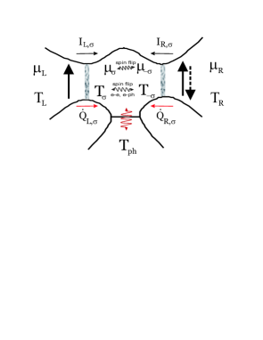
Figure 1: (Color online): Schematic spin-valve biased with a voltage and/or temperature difference. Spin-flip and inelastic electron-electron and electron-phonon scattering in the normal metal spacer lead to inter-spin energy exchange and change the thermoelectric characteristics. $I$ and $\dot{Q}$ stand for the charge and heat currents flowing into the island. $T_{\mathrm{ph}}$ is the temperature of the phonon bath.

In a spin valve (Fig. 1), a nonmagnetic island is coupled to two ferromagnetic reservoirs with parallel (P) or antiparallel (AP) magnetic alignments. The chemical potential of the left (right) reservoir is $\mu_{L(R)}$ and the temperature is $T_{L(R)}$. The conductances $G_{L/R\sigma}$ and Seebeck coefficients $S_{L/R\sigma}$ of the contacts between the island and the reservoirs depend on spin $\sigma\in\{\uparrow,\downarrow\}$. Biasing the spin valve with either a voltage $\Delta V=(\mu_{R}-\mu_{L})/e$ or a temperature difference $\Delta T=T_{R}-T_{L}$ gives rise to a spin-dependent energy distribution function $f_{\sigma}(E)$ of the electrons on the island. As shown below, in the linear response regime this can be described exactly by spin-dependent chemical potentials and temperatures, such that $f_{\sigma}(E)=f_{0}(E;\mu_{\sigma},T_{\sigma})$, where $f_{0}(E;\mu,T)=\{\exp[(E-\mu)/(k_{B}T)]+1\}^{-1}$ is the Fermi-Dirac distribution function. $\mu_{\sigma}$ and $T_{\sigma}$ are determined by conservation of charge, spin and energy (see Eqs. (2)). The response matrix of the spin valve

$$\begin{pmatrix}I\\ \dot{Q}\end{pmatrix}=\begin{pmatrix}G&GS\\ TGS&K\end{pmatrix}\begin{pmatrix}\Delta V\\ -\Delta T\end{pmatrix}$$ (1)

relates the charge and heat currents $I$ and $\dot{Q}$ to the biases $\Delta V$ and $\Delta T,$ respectively. Below, we derive expressions for the heat conductance $K$ and thermopower $S$, in the presence of inter-spin energy exchange and for different magnetic configurations.

The steady state potentials and temperatures can be determined from Kirchhoff’s laws for charge and energy for each spin.hatami For small $e\Delta V/k_{B},\Delta T\ll T_{\uparrow},T_{\downarrow}$,

$$\sum_{i=L,R}I_{i,\sigma}+G_{\mathrm{sf}}(\mu_{\sigma}-\mu_{-{\sigma}})/e=0$$ (2)

$$\sum_{i=L,R}\dot{Q}_{i,\sigma}+K^{\uparrow\downarrow}(T_{\sigma}-T_{-\sigma})+K_{\mathrm{e-ph}}(T_{\sigma}-T_{\mathrm{ph}})=0.$$

Here $I_{i,\sigma}=G_{i\sigma}(\mu_{\sigma}-\mu_{i})/e+G_{i\sigma}S_{i\sigma}(T_{\sigma}-T_{i})$ is the charge current for spin $\sigma$ through contact $i$, $Q_{i,\sigma}=\mathcal{L}_{0}G_{i\sigma}T(T_{\sigma}-T_{i})+G_{i\sigma}S_{i\sigma}T(\mu_{\sigma}-\mu_{i})/e$ is the corresponding heat current, $G_{i\sigma}$ and $S_{i\sigma}$ are the associated charge conductances and Seebeck coefficients, and $\mathcal{L}_{0}=\pi^{2}k_{B}^{2}/(3e^{2})$ is the Lorenz number. Spin decay is described by the (inter-)spin conductance $G_{\mathrm{sf}}=e^{2}\nu_{F}\Omega/\tau_{\mathrm{sf}}$ for an island with volume $\Omega$, density of states at the Fermi level $\nu_{F}$ and spin-flip relaxation time $\tau_{\mathrm{sf}}$. The term $K_{\mathrm{e-ph}}$ describes the interaction with the phonons at temperature $T_{\mathrm{ph}}$. Inter-spin energy exchange is governed by the spin heat conductance $K^{\uparrow\downarrow}=\mathcal{L}_{0}G_{\mathrm{sf}}T+K_{\mathrm{e-e}}^{\uparrow\downarrow}$, where the first term originates from the spin-flip scattering and the second is due to e-e interactions. We are allowed to discard the spatial dependence of the distribution functions when the diffusion time $\tau_{D}=L^{2}/D$ in the island with length $L$ and diffusion constant $D$ is shorter than both $\tau_{\mathrm{sf}}$ and the spin thermalization time $\tau_{\mathrm{st}}=\mathcal{L}_{0}e^{2}\nu_{F}T\Omega/(K_{\mathrm{e-ph}}+2K^{\uparrow\downarrow})$.

The in general lengthy solutions of Eqs. (2) are considerably simplified for left-right symmetric conductances and Seebeck coefficients, parameterized by $G_{0}=G_{\uparrow}+G_{\downarrow}$, $P=(G_{\uparrow}-G_{\downarrow})/G_{0}$, $S_{0}=(G_{\uparrow}S_{\uparrow}+G_{\downarrow}S_{\downarrow})/G_{0}$ and $P^{\prime}=(G_{\uparrow}S_{\uparrow}-G_{\downarrow}S_{\downarrow})/(G_{0}S_{0})$ for both junctions. In the antiparallel case the signs of $P$ and $P^{\prime}$ in one of the junctions are inverted. In the parallel configuration the heat conductance becomes

$$K_{\mathrm{P}}=\mathcal{L}_{0}G_{P}T+\frac{2K_{\mathrm{e-ph}}r(1-P^{2}\gamma)}{1-P^{2}\gamma+K_{\mathrm{e-ph}}/(\mathcal{L}_{0}G_{0}T)}$$ (3)

and in the antiparallel configuration it is

$$K_{\mathrm{AP}}=\mathcal{L}_{0}G_{P}T(1-P^{2}\gamma)+\frac{2K_{\mathrm{e-ph}}r}{1+K_{\mathrm{e-ph}}/(\mathcal{L}_{0}G_{0}T)}.$$ (4)

The factor $r=(T_{\mathrm{ph}}-T_{L})/(T_{R}-T_{L})-1/2$ parameterizes the phonon temperature on the island: If the phonons are poorly coupled to the substrate, as for example in perpendicular spin valves or in suspended structures, $T_{\mathrm{ph}}=(T_{\uparrow}+T_{\downarrow})/2$. For the P configuration this yields $r=0$, whereas for the AP configuration we get $r=-K_{\uparrow\downarrow}P/[2(K_{\mathrm{e-ph}}+K_{\uparrow\downarrow}+\mathcal{L}_{0}G_{0}T)]$. In the opposite limit $r=\pm 1/2$, viz. $T_{\mathrm{ph}}$ is fixed to the bath temperature of the left or right reservoir. The coefficient $\gamma=[1+(K_{\mathrm{e-ph}}+2K^{\uparrow\downarrow})/(\mathcal{L}_{0}G_{0}T)]^{-1}$ describes inter-spin energy exchange. Factoring out the temperature dependence of $K_{\mathrm{e-ph}}\propto T^{4}$ and $K_{\mathrm{e-e}}^{\uparrow\downarrow}\propto T^{\nu+1}$ (see the discussion below) yields $\gamma=[1+(T/T_{\mathrm{ch,ph}})^{3}+(T/T_{\mathrm{ch,e-e}})^{\nu}+2G_{\mathrm{sf}}/G_{0}]^{-1}$, where the characteristic temperatures are $T_{\mathrm{ch,e-ph}}=[(\mathcal{L}_{0}G_{0}T^{4})/K_{\mathrm{e-ph}}]^{1/3}$, $T_{\mathrm{ch,e-e}}=[(\mathcal{L}_{0}G_{0}T^{\nu+1})/(2K_{\mathrm{e-e}}^{\uparrow\downarrow})]^{1/\nu}$ for electron-phonon and electron-electron couplings, respectively. The exponent $\nu$ depends on the dimensionality ($n$d) of the sample. We are here mainly interested in 3d samples ($\nu=3/2$) in which all sample dimensions exceed the thermal coherence length $\xi_{T}=\sqrt{\hbar D/(2\pi k_{B}T)}$.

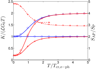
Figure 2: (Color online): Temperature dependence of the heat conductance $K$ (solid lines, left axis) and thermopower $S$ (dashed line, right axis) of a structurally left-right symmetric spin valve with $P=0.9$, $P^{\prime}=0.5$ and when the electron-phonon relaxation dominates the inter-spin energy exchange. The lines are plots of Eqs. (3)–(5) and the symbols have been calculated from the full nonequilibrium distribution function, Eqs. (10) and (11). The results have been calculated for P configuration with $r=0$ (circles) and $r=1/2$ (squares) and AP configuration with $r=0$ (stars) and $r=1/2$ (triangles).

In the parallel configuration the thermopower satisfies $S_{\mathrm{P}}=S_{0}$ and in the antiparallel onenophononterm

$$\frac{S_{\mathrm{AP}}}{S_{\mathrm{P}}}=\frac{1-PP^{\prime}+2G_{\mathrm{sf}}/G_{0}+\gamma P\left(P-P^{\prime}-2P^{\prime}G_{\mathrm{sf}}/G_{0}\right)}{1-P^{2}+2G_{\mathrm{sf}}/G_{0}}.$$ (5)

The temperature dependence of $K$ and $S$ is plotted in Fig. 2 for $K_{\mathrm{e-ph}}\gg K_{\mathrm{e-e}},\mathcal{L}_{0}G_{\mathrm{sf}}T$. For $T\ll\min(T_{\rm ch,e-e},T_{\rm ch,e-ph})\equiv T_{\rm ch}$, the device operates as a spin heat valve in which the heat current can be controlled by the magnetization configuration. Contrary to the charge conductance, however, the magnetoheat conductance $(K_{\mathrm{P}}-K_{\mathrm{AP}})/K_{\mathrm{P}}$ vanishes for $T\gg T_{\rm ch}$ or $\gamma\rightarrow 0$. Thus the presence of inelastic scattering leads to a violation of the Wiedemann-Franz law $K=\mathcal{L}_{0}GT$ for $T\gtrsim T_{\rm ch}$. The magnetothermopower $(S_{\mathrm{P}}-S_{\mathrm{AP}})/S_{\mathrm{P}}$ persists provided $P\neq P^{\prime}$.hatami The measured heat conductance and thermopower as a function of temperature and magnetic configuration may hence yield unprecedented information on the energy relaxation in normal metals.

We now address the characteristic temperatures $T_{\mathrm{ch,e-ph}}$ and $T_{\mathrm{ch,e-e}}$. The former can be obtained directly from the Debye form for the heat conductance between electrons and acoustic phonons,wellstood94 $K_{\mathrm{e-ph}}=\frac{5}{2}\Sigma\Omega T^{4}$, valid for $T\ll T_{\mathrm{Debye}}$. Here $\Sigma$ is the e-ph coupling constantgiazotto06 and the factor $1/2$ takes into account spin degeneracy. The characteristic temperature for electron-phonon coupling thus reads

$$T_{\mathrm{ch,e-ph}}=\left(\frac{\pi k_{B}^{2}}{15\hbar\Sigma\Omega}\right)^{1/3}\left(\frac{G_{0}h}{e^{2}}\right)^{1/3}.$$ (6)

For $T\gtrsim T_{\mathrm{Debye}}$, the electron – acoustic phonon scattering and thereby inter-spin energy exchange saturates. Optical phonons start to contribute in this temperature regime, but are disregarded here.

The e-e scattering collision integrals with spin-dependent distribution functions contain three terms

$$I_{\mathrm{e-e},\sigma}(\epsilon)=I_{\mathrm{(a)}}^{\sigma\sigma}(\epsilon)+I_{\mathrm{(b)}}^{\sigma,-{\sigma}}(\epsilon)+I_{\mathrm{(c)}}^{\sigma,-{\sigma}}(\epsilon),$$

presented by the diagrams in Fig. 3.

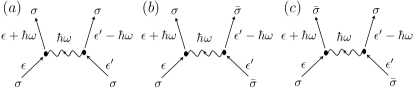
Figure 3: Electron-electron scattering vertices. (a) Equal-spin scattering, which equilibrates the electrons but does not thermalize the spins. (b) Spin conserving scattering and (c) spin exchange scattering, which do thermalize the spins.

Processes (b) and (c) induce inter-spin energy exchange, which can be described in terms of a heat current flowing between two spin ensembles,giazotto06

$$\dot{Q}_{\mathrm{e-e}}^{\uparrow\downarrow}=\nu_{F}\Omega\int d\epsilon\epsilon(I_{\mathrm{(b)}}^{\uparrow\downarrow}+I_{\mathrm{(c)}}^{\uparrow\downarrow}).$$ (7)

The direct spin current due to e-e interaction vanishes in the absence of spin-orbit scattering, $\int d\epsilon(I_{\mathrm{(a)}}^{\uparrow\downarrow}+I_{\mathrm{(b)}}^{\uparrow\downarrow}+I_{\mathrm{(c)}}^{\uparrow\downarrow})=0.$ In 3d, to lowest order in spin particle and heat accumulation, $\left(\mu_{\uparrow}-\mu_{\downarrow}\right)/\left(\mu_{\uparrow}+\mu_{\downarrow}\right)\ll 1$ and $T_{s}/(T_{\uparrow}+T_{\downarrow})\ll 1$, we arrive at $\dot{Q}_{\mathrm{e-e}}^{\uparrow\downarrow}\approx(K_{(b)}^{\uparrow\downarrow}+K_{(c)}^{\uparrow\downarrow})(T_{\uparrow}-T_{\downarrow})$, where

$$K_{(b)}^{\uparrow\downarrow} =\frac{105\zeta(7/2)k_{B}^{7/2}T^{5/2}}{32[2\pi E_{T}(1+F)]^{3/2}\hbar},$$ (8a)

$$K_{(c)}^{\uparrow\downarrow} =\frac{FC}{(F+2)}\frac{[\pi^{2}\zeta(3/2)+\frac{35}{16}\zeta(7/2)]k_{B}^{7/2}T^{5/2}}{2[2\pi E_{T}(F+1)]^{3/2}\hbar}.$$ (8b)

Here $C=-1+(F+1)^{3/2}$, $F>-1$ is the spin triplet Fermi liquid parameter ($F=-1$ corresponds to the Stoner instability), $E_{T}=\hbar D/\Omega^{2/3}$ is the Thouless energy proportional to the inverse time it takes to diffuse over a length $\Omega^{1/3}$ and $\zeta(x)$ is the Zeta function. Summing the two contributions from Eqs. (8) yields the characteristic temperature

$$T_{\mathrm{ch,e-e}}=8\pi\left(\frac{G_{0}h}{e^{2}}\right)^{2/3}\frac{E_{T}}{k_{B}}(F+1)\times$$ (9)

$$\left\{\frac{\pi(F+2)}{48FC\pi^{2}\zeta(3/2)+105[6+F(3+C)]\zeta(7/2)}\right\}^{2/3}.$$

In 1d and 2d structures the spin-flip contribution (c) has an infrared divergencedimitrova07 ; chtchelkatchev08 that needs to be regularized. As a result, the inter-spin energy exchange due to e-e scattering becomes stronger and the corresponding $T_{\mathrm{ch,e-e}}$ lower. This is especially relevant at low temperatures and small structures since $\xi_{T}$ may exceed 100 nm at $T\approx$ 1 K. We intend to analyze the resulting inter-spin energy exchange in reduced dimensions in the future.

In order to assess the relevance of our results for realistic samples we consider a disordered island of a spin valve coupled to the reservoirs via tunnel contacts. For example, with $F=-0.3$ we get

$$T_{\mathrm{ch,e-e}} \approx 0.9\text{ }\operatorname{K}\times\frac{D}{0.001\text{ }\operatorname{m}^{2}/\text{s}}\left[\frac{0.1\text{ }(\operatorname{\mu m})^{3}}{\Omega}\frac{G_{0}}{0.01\operatorname{S}}\right]^{2/3}$$

$$T_{\mathrm{e-ph}} \approx 1\text{ }\operatorname{K}\times\left[\frac{10^{9}\text{ }\operatorname{W}\operatorname{m}^{-3}\operatorname{K}^{-5}}{\Sigma}\frac{0.1\text{ }(\operatorname{\mu m})^{3}}{\Omega}\frac{G_{0}}{0.01\operatorname{S}}\right]^{1/3}.$$

Making the sample smaller and conductance larger increases both characteristic temperatures, but the increase for $T_{\mathrm{ch,e-ph}}$ is slower. For $\Omega=0.001$ ($\operatorname{\mu m}$)³ and $G_{0}=1$ $\operatorname{S}$ we get $T_{\mathrm{ch,e-ph}}=22$ $\operatorname{K}$ whereas $T_{\mathrm{cr,e-e}}=400$ $\operatorname{K}$. We may therefore conclude that in spin valves with metallic contacts and 3d spacers the inter-spin energy exchange due to e-e interaction can be neglected. The spin thermalization rate with $F=-0.3$ is

$$\frac{1}{\tau_{\mathrm{st}}}\approx\bigg{[}\frac{1}{20\mathrm{\operatorname{ns}}}\left(\frac{T}{1\operatorname{K}}\right)^{3/2}\left(\frac{0.001\operatorname{m}\mathrm{{}^{2}/s}}{D}\right)^{3/2}+$$

$$\frac{1}{25\mathrm{\operatorname{ns}}}\left(\frac{T}{1\operatorname{K}}\right)^{3}\left(\frac{\Sigma}{10^{9}\text{ }\operatorname{W}\operatorname{m}^{-3}\operatorname{K}^{-5}}\right)\bigg{]}\times\frac{10^{47}\text{ }\operatorname{J}^{-1}\text{ }\operatorname{m}^{-3}}{\nu_{F}}.$$

The first term comes from e-e scattering and the second from e-ph scattering. This rate exceeds the spin-flip scattering rate $\sim 10$ $\operatorname{GHz}$ at temperatures above $\sim 10$ $\operatorname{K}$.

Above we assume that the electron energy distribution function is well represented by Fermi-Dirac distributions with spin-dependent chemical potentials and temperatures. This is not true in general, since $f_{\sigma}(\epsilon)$ has the nonequilibrium formgiazotto06 ; pothier97

$$f_{\sigma}(\epsilon)=\frac{G_{L\sigma}f_{L}+G_{R\sigma}f_{R}+\nu_{F}e^{2}\Omega I_{\mathrm{coll}}[f_{\sigma},f_{-{\sigma}}]}{G_{L\sigma}+G_{R\sigma}},$$ (10)

where $f_{L/R}=f_{0}(\epsilon;\mu_{L/R},T)$ are the distribution functions for the reservoirs and $I_{\mathrm{coll}}$ describes all inelastic scattering events. The charge ($n=0$) and heat ($n=1$) currents through contact $i$ then become

$$I_{i}|\dot{Q}_{i}=\sum_{\sigma}\int d\epsilon(\epsilon-\mu_{i})^{n}\frac{G_{i\sigma}}{e^{1+n}}(\epsilon)(f_{\sigma}(\epsilon)-f_{i}(\epsilon)).$$ (11)

Thermoelectric effects can be included by adding a weak energy dependence to the conductances, $G_{i\sigma}(\epsilon)\approx G_{i\sigma}^{0}[1+c_{i\sigma}(\epsilon-\mu_{i})]$, and expanding to linear order in $c_{i,\sigma}$. Identifying $S_{i\sigma}=e\mathcal{L}_{0}c_{i\sigma}T$, we recover Eqs. (4) and (5) in the regime $e\Delta V/k_{B},\Delta T\ll T_{L},T_{R}\approx T$ even in the absence of collisions (i.e., $\gamma=1$).   For $c_{i\sigma}=0$ and to linear order in the applied bias, the nonequilibrium distribution (10) is identical to the quasiequilibrium one. Under these conditions, the collision integrals can be calculated by replacing the full distribution functions by the quasiequilibrium ones. Numerical solutions of the kinetic equations (see Fig. 2) indicate that in linear response collisions and finite $c_{i\sigma}$’s do not change this conclusion.

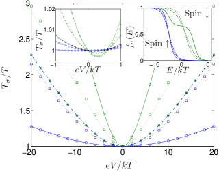
Figure 4: (Color online): Spin-dependent effective temperature vs. voltage in an asymmetric spin valve with $P=0.9$, $P^{\prime}=0.5$ and $G_{R}=0.1G_{L}$. The lines are calculated from Eqs. (2) and (13) and the symbols from Eq. (12) for numerical solutions of the kinetic equations. The upper curves are for majority, the lower for minority spins, and different strengths of e-e scattering with $F=0$: no scattering (solid line and circles), weak scattering with $E_{T}=0.05k_{B}T$ and $G_{L}=100e^{2}/h$ (dashed line and squares), and strong scattering with $E_{T}=0.001k_{B}T$ and $G_{L}=100e^{2}/h$ (dash-dotted line and stars). Here $T$ denotes the temperature of the reservoirs. Left inset: behavior at low bias with thermoelectric effects $c_{L}=10c_{R}=0.02/(kT)$. Right inset: distribution function at $e\Delta V=10E_{T}$ with different strengths of e-e scattering.

Beyond linear response spin-dependent temperatures can strictly speaking be invoked only in the presence of strong inelastic scattering such that $T_{\uparrow}\approx T_{\downarrow}$. Nevertheless we can define effective electron temperatures that satisfy the standard relation with the thermal energy density in the Sommerfeld expansion:ashcroftmermin

$$T_{\sigma}=\frac{\sqrt{6}}{\pi k_{B}}\sqrt{\int_{-\infty}^{\infty}[f_{\sigma}(\epsilon)-1+\theta(\epsilon-\mu_{\sigma})]\epsilon d\epsilon}.$$ (12)

Proceeding with Fermi-Dirac distributions with effective spin-dependent temperatures and chemical potentials, $\mu_{\sigma}$ and $T_{\sigma}$ can be obtained from Eqs. (2) by replacing the expression for the charge and heat currents through contact $i$ with their nonlinear counterparts,

$$I_{\sigma}=\frac{G_{i,\sigma}}{e}\left\{\mu_{\sigma}-\mu_{i}+\frac{c_{i\sigma}}{2}\left[\mathcal{L}_{0}e^{2}(T_{\sigma}^{2}-T_{i}^{2})-(\mu_{\sigma}-\mu_{i})^{2}\right]\right\}$$

$$\dot{Q}_{i,\sigma}=G_{i,\sigma}\left[\mathcal{L}_{0}(T_{\sigma}^{2}-T_{i}^{2})/2-(\mu_{\sigma}^{2}-\mu_{i}^{2})/(2e^{2})\right]$$ (13)

$$+G_{i\sigma}c_{i\sigma}(\mu_{\sigma}-\mu_{i})\left[\mathcal{L}_{0}(T_{\sigma}^{2}+T_{i}^{2})/2-(\mu_{\sigma}^{2}-\mu_{i}^{2})/(6e^{2})\right].$$

These equations are obtained by a direct integration of Eq. (11) using Fermi-Dirac functions $f_{i}(\epsilon)$ and $f_{\sigma}(\epsilon)$. We also have to replace the linear-response forms of the spin mixing terms in Eqs. (2) by their forms far from equilibrium. For example, for e-e scattering with $F=0$ we use $\dot{Q}^{\sigma\bar{\sigma}}=15\zeta(7/2)k_{B}^{7/2}(T_{\sigma}^{7/2}-T_{-{\sigma}}^{7/2})/[16\hbar(2\pi E_{T})^{3/2}]$.

In the absence of collisions and for weak thermoelectric effects it can be proven by direct integration that the effective temperatures defined by Eq. (12) agree with those which follow from heat conservation. In Fig. 4 we present a complete numerical solution of the kinetic equations along with the results from the quasiequilibrium heat balance equations from which we conclude that the two approaches for calculating $T_{\sigma}$ agree also in the presence of inter-spin energy exchange.

Spin heat accumulation cannot be directly measured by two-terminal transport experiments in linear systems. In order to prove the presence of a sizable $T_{s}$ far from equilibrium it should be probed by spin-selective thermometry, such as a generalization of the tunnel-spectroscopy in Ref. pothier97, , by measuring the shot noise of the spin valve, or through electron spin resonance.

In conclusion, we have shown that inter-spin energy exchange in a spin valve affects the temperature and magnetic configuration dependence of its thermoelectric properties. The different thermalization mechanisms can be quantified by characteristic temperatures, Eqs. (6) and (9), above which interaction effects become important. We introduce the concept of spin heat accumulation via the spin-dependent effective electron temperatures $T_{\sigma}$ in Fermi-Dirac distribution functions, which can be used to describe transport properties beyond the linear response regime. We demarcate the regime in which spin valves can be employed to control heat currents. Other types of operations can be envisaged as well, such as spin-selective cooling of the electrons (see the left inset of Fig. 4).

We thank P. Virtanen for discussions. This work was supported by the Academy of Finland, the Finnish Cultural Foundation, and NanoNed, a nanotechnology programme of the Dutch Ministry of Economic Affairs. TTH acknowledges the hospitality of Delft University of Technology, where this work was initiated.