Eigenvalue method to compute the largest relaxation time of disordered systems

Abstract

We consider the dynamics of finite-size disordered systems as defined by a master equation satisfying detailed balance. The master equation can be mapped onto a Schrödinger equation in configuration space, where the quantum Hamiltonian $H$ has the generic form of an Anderson localization tight-binding model. The largest relaxation time $t_{eq}$ governing the convergence towards Boltzmann equilibrium is determined by the lowest non-vanishing eigenvalue $E_{1}=1/t_{eq}$ of $H$ (the lowest eigenvalue being $E_{0}=0$). So the relaxation time $t_{eq}$ can be computed without simulating the dynamics by any eigenvalue method able to compute the first excited energy $E_{1}$. Here we use the ’conjugate gradient’ method to determine $E_{1}$ in each disordered sample and present numerical results on the statistics of the relaxation time $t_{eq}$ over the disordered samples of a given size for two models : (i) for the random walk in a self-affine potential of Hurst exponent $H$ on a two-dimensional square of size $L\times L$, we find the activated scaling $\ln t_{eq}(L)\sim L^{\psi}$ with $\psi=H$ as expected; (ii) for the dynamics of the Sherrington-Kirkpatrick spin-glass model of $N$ spins, we find the growth $\ln t_{eq}(N)\sim N^{\psi}$ with $\psi=1/3$ in agreement with most previous Monte-Carlo measures. In addition, we find that the rescaled distribution of $(\ln t_{eq})$ decays as $e^{-u^{\eta}}$ for large $u$ with a tail exponent of order $\eta\simeq 1.36$. We give a rare-event interpretation of this value, that points towards a sample-to-sample fluctuation exponent of order $\psi_{width}\simeq 0.26$ for the barrier.

I Introduction

The non-equilibrium dynamics of disordered systems has been much studied both experimentally and theoretically (see for instance the reviews [1, 2] and references therein). In numerical simulations, the main limitation is that the equilibrium time $t_{eq}(L)$ needed to converge towards equilibrium for a finite system of linear size $L$ grows very rapidly with $L$. Within the droplet scaling theory proposed both for spin-glasses [3, 4] and for the directed polymer in a random medium [5], the non-equilibrium dynamics is activated with barriers scaling as a power law $B(L)\sim L^{\psi}$ with some barrier exponent $\psi>0$ that is independent of temperature and disorder strength. The equilibrium time $t_{eq}(L)$ then grows as

$$\ln t_{eq}(L)=B(L)\sim L^{\psi}$$ (1)

This logarithmic scaling has been used to fit numerical data for disordered ferromagnets [6, 7, 8] and spin-glasses [9, 10]. Other authors, both for disordered ferromagnets [11, 12] and spin-glasses [13, 14] prefer a scenario corresponding to logarithmic barriers $B(L)\sim z(T,\epsilon)\ln L$, so that the equilibrium time $t_{eq}(L)$ scales as a power-law

$$t_{eq}(L)=e^{B(L)}\sim L^{z(T,\epsilon)}$$ (2)

where the exponent $z(T,\epsilon)$ is non-universal and depends on the temperature $T$ as well as on the disorder strength $\epsilon$. In the field of directed polymers or elastic lines in random media, the fit based the algebraic form of Eq. 2 used initially by many authors [15] has been now excluded by more recent work [16, 17, 18], and has been interpreted as an artefact of an initial transient regime [17, 18]. The reason why the debate between the two possibilities of Eqs 1 and 2 has remained controversial over the years for many interesting disordered models is that the equilibrium time $t_{eq}(L)$ grows numerically so rapidly with $L$ that $t_{eq}(L)$ can be reached at the end of dynamical simulations only for rather small system sizes $L\leq L_{max}$. For instance, in Monte-Carlo simulations of 2D or 3D random ferromagnets [6, 7, 8, 11, 12, 19] or spin-glasses [9, 10, 13, 14], the maximal equilibrated size is usually only of order $L_{max}\sim 10$ lattice spacings. Even faster-than-the-clock Monte Carlo algorithms [20], where each iteration leads to a movement, become inefficient because they face the ’futility’ problem [21] : the number of different configurations visited during the simulation remains very small with respect to the accepted moves, i.e. the system visits over and over again the same configurations within a given valley before it is able to escape towards another valley. A recent proposal to improve significantly Monte Carlo simulations of disordered systems consists in introducing some renormalization ideas [22].

Taking into account these difficulties, a natural question is whether it could be possible to obtain informations on the equilibrium time $t_{eq}(L)$ without simulating the dynamics. In previous works [23, 24], we have proposed for instance to study the flow of some strong disorder renormalization procedure acting on the transitions rates of the master equation. However this approach is expected to become asymptotically exact only if the probability distribution of renormalized transitions rates flows towards an ’infinite disorder’ fixed point, i.e. only for the activated scaling of Eq. 1. In the present paper, we test another strategy to compute $t_{eq}$ which is a priori valid for any dynamics defined by a master equation satisfying detailed balance : it is based on the computation of the first excited energy $E_{1}$ of the quantum Hamiltonian $H$ that can be associated to the master equation. This approach makes no assumption on the nature of the dynamics and is thus valid both for activated or non-activated dynamics (Eqs 1 or 2). The mapping between continuous-time stochastic dynamics with detailed balance and quantum Schrödinger equations is of course very well-known and can be found in most textbooks on stochastic processes (see for instance [25, 26, 27]). However, since it is very often explained on special cases, either only in one-dimension, or only for continuous space, or only for Fokker-Planck equations, we stress here that this mapping is valid for any master equation satisfying detailed balance (see more details in section II). In the field of disordered systems, this mapping has been very much used for one-dimensional models (see the review [28] and references therein, as well as more recent works [29, 30, 31]), but to the best of our knowledge, it has not been used in higher dimension, nor for many-body problems. In the field of many-body dynamics without disorder, this mapping has been already used as a numerical tool to measure very precisely the dynamical exponent $z$ of the two dimensional Ising model at criticality [32].

The paper is organized as follows. In section II, we recall how the master equation can be mapped onto a Schrödinger equation in configuration space, and describe how the equilibrium time $t_{eq}$ can be obtained from the associated quantum Hamiltonian. We then apply this method to two types of disordered models : section III concerns the problem of a random walk in a two-dimensional self-affine potential, and section IV is devoted to the the dynamics of the Sherrington-Kirkpatrick spin-glass model. Our conclusions are summarized in section Acknowledgements.

II Quantum Hamiltonian associated to the Master Equation

II.1 Master Equation satisfying detailed balance

In statistical physics, it is convenient to consider continuous-time stochastic dynamics defined by a master equation of the form

$$\frac{dP_{t}\left({\cal C}\right)}{dt}=\sum_{\cal C^{\prime}}P_{t}\left({\cal C}^{\prime}\right)W\left({\cal C}^{\prime}\to{\cal C}\right)-P_{t}\left({\cal C}\right)W_{out}\left({\cal C}\right)$$ (3)

that describes the the evolution of the probability $P_{t}({\cal C})$ to be in configuration ${\cal C}$ at time t. The notation $W\left({\cal C}^{\prime}\to{\cal C}\right)$ represents the transition rate per unit time from configuration ${\cal C}^{\prime}$ to ${\cal C}$, and

$$W_{out}\left({\cal C}\right)\equiv\sum_{{\cal C}^{\prime}}W\left({\cal C}\to{\cal C}^{\prime}\right)$$ (4)

represents the total exit rate out of configuration ${\cal C}$. Let us call $U(C)$ the energy of configuration ${\cal C}$. To ensure the convergence towards Boltzmann equilibrium at temperature $T$ in any finite system

$$P_{eq}({\cal C})=\frac{e^{-\frac{U({\cal C})}{T}}}{Z}$$ (5)

where $Z$ is the partition function

$$Z=\sum_{\cal C}e^{-\frac{U({\cal C})}{T}}$$ (6)

it is sufficient to impose the detailed-balance property

$$e^{-\frac{U({\cal C})}{T}}W\left(\cal C\to\cal C^{\prime}\right)=e^{-\frac{U({\cal C^{\prime}})}{T}}W\left(\cal C^{\prime}\to\cal C\right)$$ (7)

II.2 Mapping onto a Schrödinger equation in configuration space

As is well known (see for instance [25, 26, 27]) the master equation operator can be transformed into a symmetric operator via the change of variable

$$P_{t}({\cal C})\equiv e^{-\frac{U(\cal C)}{2T}}\psi_{t}({\cal C})$$ (8)

The function $\psi_{t}({\cal C})$ then satisfies an imaginary-time Schrödinger equation

$$\frac{d\psi_{t}\left({\cal C}\right)}{dt}=-H\psi_{t}\left({\cal C}\right)$$ (9)

where the quantum Hamiltonian has the generic form of an Anderson localization model in configuration space

$$H=\sum_{\cal C}\epsilon\left({\cal C}\right)|{\cal C}><{\cal C}|+\sum_{{\cal C},{\cal C^{\prime}}}V({\cal C},{\cal C^{\prime}})|{\cal C}><{\cal C^{\prime}}|$$ (10)

The on-site energies read

$$\epsilon\left({\cal C}\right)=W_{out}\left({\cal C}\right)$$ (11)

whereas the hopping terms read

$$V({\cal C},{\cal C^{\prime}})=-e^{-\frac{(U(\cal C^{\prime})-U(\cal C))}{2T}}W\left(\cal C^{\prime}\to\cal C\right)$$ (12)

II.3 Specific choices for the detailed balance dynamics

To have the detailed balance of Eq. 7, it is convenient to rewrite the rates in the following form

$$W\left(\cal C\to\cal C^{\prime}\right)=\delta_{<\cal C,\cal C^{\prime}>}\ e^{-\frac{(U({\cal C^{\prime}})-U({\cal C}))}{2T}}e^{-S(\cal C,\cal C^{\prime})}$$ (13)

where $\delta_{<\cal C,\cal C^{\prime}>}$ means that the two configurations are related by an elementary dynamical move, and where $S(\cal C,\cal C^{\prime})$ is an arbitrary symmetric function : $S(\cal C,\cal C^{\prime})=S(\cal C^{\prime},\cal C)$.

II.3.1 Simplest choice $S({\cal C,\cal C^{\prime}})=0$

To have the detailed balance property of Eq. 7, the simplest choice in Eq. 13 corresponds to $S({\cal C,\cal C^{\prime}})=0$

$$W\left(\cal C\to\cal C^{\prime}\right)=\delta_{<\cal C,\cal C^{\prime}>}\ e^{-\frac{(U({\cal C^{\prime}})-U({\cal C}))}{2T}}$$ (14)

Then the hopping terms of the quantum Hamiltonian are simply

$$V({\cal C},{\cal C^{\prime}})=-\delta_{<\cal C,\cal C^{\prime}>}$$ (15)

i.e. the non-vanishing hopping terms are not random, but take the same constant value $(-1)$ as in usual Anderson localization tight binding models. The on-site energies are random and read

$$\epsilon\left({\cal C}\right)=\sum_{\cal C^{\prime}}\delta_{<\cal C,\cal C^{\prime}>}\ e^{-\frac{(U(\cal C^{\prime})-U(\cal C))}{2T}}$$ (16)

II.3.2 Metropolis choice

In numerical simulations, one of the most frequent choice corresponds to the Metropolis transition rates

$$W\left(\cal C\to\cal C^{\prime}\right)=\delta_{<\cal C,\cal C^{\prime}>}{\rm min}\left[1,e^{-\frac{(U({\cal C^{\prime}})-U({\cal C}))}{T}}\right]$$ (17)

In Eq. 13, this corresponds to the choice

$$S({\cal C,\cal C^{\prime}})=\frac{|U({\cal C^{\prime}})-U({\cal C})|}{2T}$$ (18)

In the quantum Hamiltonian, the hopping terms then read

$$V^{metropolis}({\cal C},{\cal C^{\prime}})=-\delta_{<\cal C,\cal C^{\prime}>}e^{-\frac{|U({\cal C^{\prime}})-U({\cal C})|}{2T}}$$ (19)

and the on-site energies are given by

$$\epsilon^{metropolis}\left({\cal C}\right)=\sum_{\cal C^{\prime}}\delta_{<\cal C,\cal C^{\prime}>}\ {\rm min}\left[1,e^{-\frac{(U({\cal C^{\prime}})-U({\cal C}))}{T}}\right]$$ (20)

II.4 Properties of the spectrum of the quantum Hamiltonian $H$

Let us note $E_{n}$ the eigenvalues of $H$ and $|\psi_{n}>$ the associated normalized eigenvectors

$$H|\psi_{n}> =E_{n}|\psi_{n}>$$ (21)

$$\sum_{\cal C}|\psi_{n}({\cal C})|^{2} =1$$ (22)

The decomposition onto these eigenstates of the evolution operator $e^{-tH}$

$$<{\cal C}|e^{-tH}|{\cal C}_{0}>=\sum_{n}e^{-E_{n}t}\psi_{n}({\cal C})\psi_{n}^{*}({\cal C}_{0})$$ (23)

yields the following expansion for the conditional probability $P_{t}\left({\cal C}|{\cal C}_{0}\right)$ to be in configuration ${\cal C}$ at $t$ if one starts from the configuration ${\cal C}_{0}$ at time $t=0$

$$P_{t}\left({\cal C}|{\cal C}_{0}\right)=e^{-\frac{U({\cal C})-U({\cal C}_{0})}{2T}}<{\cal C}|e^{-tH}|{\cal C}_{0}>=e^{-\frac{U({\cal C})-U({\cal C}_{0})}{2T}}\sum_{n}e^{-E_{n}t}\psi_{n}({\cal C})\psi_{n}^{*}({\cal C}_{0})$$ (24)

The quantum Hamiltonian $H$ has special properties that come from its relation to the dynamical master equation :

(i) the ground state energy is $E_{0}=0$, and the corresponding eigenvector is given by

$$\psi_{0}({\cal C})=\frac{e^{-\frac{U({\cal C})}{2T}}}{\sqrt{Z}}$$ (25)

where $Z$ is the partition function of Eq. 6.

This corresponds to the convergence towards the Boltzmann equilibrium in Eq. 8 for any initial condition ${\cal C}_{0}$

$$P_{t}\left({\cal C}|{\cal C}_{0}\right)\mathop{\simeq}_{t\to+\infty}e^{-\frac{U({\cal C})-U({\cal C}_{0})}{2T}}\psi_{0}({\cal C})\psi_{0}^{*}({\cal C}_{0})=\frac{e^{-\frac{U({\cal C})}{T}}}{Z}=P_{eq}({\cal C})$$ (26)

(ii) the other energies $E_{n}>0$ determine the relaxation towards equilibrium. In particular, the lowest non-vanishing energy $E_{1}$ determines the largest relaxation time $(1/E_{1})$ of the system

$$P_{t}\left({\cal C}|{\cal C}_{0}\right)-P_{eq}({\cal C})\mathop{\simeq}_{t\to+\infty}e^{-E_{1}t}e^{-\frac{U({\cal C})-U({\cal C}_{0})}{2T}}\psi_{1}({\cal C})\psi_{1}^{*}({\cal C}_{0})$$ (27)

Since this largest relaxation time represents the ’equilibrium time’, i.e. the characteristic time needed to converge towards equilibrium, we will use the following notation from now on

$$t_{eq}\equiv\frac{1}{E_{1}}$$ (28)

The conclusion of this section is thus that the relaxation time $t_{eq}$ can be computed without simulating the dynamics by any eigenvalue method able to compute the first excited energy $E_{1}$ of the quantum Hamiltonian $H$ (where the ground state is given by Eq. 25 and has for eigenvalue $E_{0}=0$). In the following subsection, we describe one of such methods called the ’conjugate gradient’ method.

II.5 Conjugate gradient method in each sample to compute $E_{1}$

The ’conjugate gradient method’ has been introduced as an iterative algorithm to find the minimum of functions of several variables with much better convergence properties than the ’steepest descent’ method [33, 34]. It can be applied to find the ground state eigenvalue and the associated eigenvector by minimizing the corresponding Rayleigh quotient [35, 36]

$$R\equiv\frac{<v|H|v>}{<v|v>}$$ (29)

The relation with the Lanczos method to solve large sparse eigenproblems is discussed in the chapters 9 and 10 of the book [34]. In the following, we slightly adapt the method described in [35, 36] concerning the ground state $E_{0}$ to compute instead the first excited energy $E_{1}$ : the only change is that the Rayleigh quotient has to be minimized within the space orthogonal to the ground state.

In the remaining of this paper, we apply this method to various disordered models to obtain the probability distribution of the equilibrium time $t_{eq}(L)$ over the samples of a given size $L$. More precisely, since the appropriate variable is actually the equilibrium barrier defined as

$$\Gamma_{eq}\equiv\ln t_{eq}=-\ln E_{1}$$ (30)

we will present numerical results for the probability distribution $Q_{L}(\Gamma_{eq})$ for various sizes $L$.

III Random walk in a two-dimensional self-affine potential

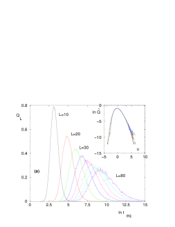
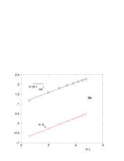
Figure 1: (Color on line) Statistics of the equilibrium time $t_{eq}$ over the disordered samples of sizes $L^{2}$ for the random walk in a two-dimensional self-affine random potential of Hurst exponent $H=0.5$ : (a) Probability distribution $Q_{L}(\Gamma_{eq}=\ln t_{eq})$ for $L=10,20,30,40,50,60,70,80$ (Inset : the corresponding distributions $\tilde{Q}(u)$ of the rescaled variable $u\equiv(\Gamma_{eq}-\overline{\Gamma_{eq}}(L))/\Delta(L)$ are shown in log scale for $L=10,20,30,40$); (b) the log-log plots of the disorder-average $\overline{\Gamma_{eq}}(L)=\overline{\ln t_{eq}}(L)$ and of the width $\Delta(L)$ corresponds to the barrier exponent $\psi=H=0.5$ (Eq. 34)

In this section, we apply the method of the previous section to the continuous-time random walk of a particle in a two-dimensional self-affine quenched random potential of Hurst exponent $H=0.5$. Since we have studied recently in [24] the very same model via some strong disorder renormalization procedure, we refer the reader to [24] and references therein for a detailed presentation of the model and of the numerical method to generate the random potential. Here we simply recall what is necessary for the present approach.

We consider finite two-dimensional lattices of sizes $L\times L$. The continuous-time random walk in the random potential $U(\vec{r})$ is defined by the master equation

$$\frac{dP_{t}\left({\vec{r}}\right)}{dt}=\sum_{\vec{r}\ ^{\prime}}P_{t}\left({\vec{r}}\ ^{\prime}\right)W\left({\vec{r}}\ ^{\prime}\to{\vec{r}}\right)-P_{t}\left({\vec{r}}\right)W_{out}\left({\vec{r}}\right)$$ (31)

where the transition rates are given by the Metropolis choice at temperature $T$ (the numerical data presented below correspond to $T=1$)

$$W\left(\vec{r}\to\vec{r}\ ^{\prime}\right)=\delta_{<\vec{r},\vec{r}\ ^{\prime}>}\ {\rm min}\left(1,e^{-(U(\vec{r}\ ^{\prime})-U(\vec{r}))/T}\right)$$ (32)

where the factor $\delta_{<\vec{r},\vec{r}\ ^{\prime}>}$ means that the two positions are neighbors on the two-dimensional lattice. The random potential $U(\vec{r})$ is self-affine with Hurst exponent $H=0.5$

$$\overline{\left[U(\vec{r})-U(\vec{r}\ ^{\prime})\right]^{2}}\mathop{\simeq}_{|\vec{r}-\vec{r}\ ^{\prime}|\to\infty}|\vec{r}-\vec{r}\ ^{\prime}|^{2H}$$ (33)

On Fig. 1 (a), we show the corresponding probability distribution $Q_{L}(\Gamma_{eq})$ for various sizes $10\leq L\leq 80$ with a statistics of $36.10^{5}\geq n_{s}(L)\geq 4.10^{4}$ disordered samples.

As shown by the log-log plots of Fig. 1 (b), we find that the disorder-averaged value ${\overline{\Gamma}_{eq}(L)}$ and the width $\Delta(L)$ of the distribution $Q_{L}(\Gamma_{eq})$ of the equilibrium barrier of Eq. 30 involve the barrier exponent $\psi$

$$\overline{\Gamma_{eq}}(L) \mathop{\propto}_{L\to\infty}L^{\psi}$$

$$\Delta(L) \mathop{\propto}_{L\to\infty}L^{\psi}$$ (34)

of value

$$\psi=H=0.5$$ (35)

These results are in agreement with scaling arguments on barriers [37, 28] and with the strong disorder renormalization approach of [24].

IV Dynamics of the Sherrington-Kirkpatrick spin-glass model

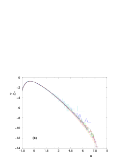
Figure 2: (Color on line) Statistics of the equilibrium time $t_{eq}$ over the disordered samples for the Sherrington-Kirkpatrick spin-glass model of $N$ spins ($2^{N}$ configurations) : (a) the log-log plot of the disorder-average $\overline{\Gamma_{eq}}(L)$ as a function of $N$ for $6\leq N\leq 20$ corresponds to the barrier exponent $\psi=1/3$ (Eq. 41) (b) The rescaled probability distribution ${\tilde{Q}}(u)$ of Eq. 44, shown here for $8\leq N\leq 16$, in log scale to see the tail of Eq. 45 : the tail exponent is of order $\eta\simeq 1.36$.

As an example of application to a many-body disordered system, we consider in this section the of the Sherrington-Kirkpatrick spin-glass model where a configuration ${\cal C}=\{S_{i}\}$ of $N$ spins $S_{i}=\pm 1$ has for energy [38]

$$U=-\sum_{1\leq i<j\leq N}J_{ij}S_{i}S_{j}$$ (36)

where the couplings are random quenched variables of zero mean $\overline{J}=0$ and of variance $\overline{J^{2}}=1/(N-1)$. The Metropolis dynamics corresponds to the master equation of Eq. 3 in configuration space with the transition rates

$$W\left({\cal C}\to{\cal C}^{\prime}\right)=\delta_{<{\cal C},{\cal C}\ ^{\prime}>}\ {\rm min}\left(1,e^{-(U({\cal C}\ ^{\prime})-U({\cal C}))/T}\right)$$ (37)

where the factor $\delta_{<{\cal C},{\cal C}\ ^{\prime}>}$ means that the two configurations are related by a single spin flip. The data presented below correspond to the temperature $T=0.5=T_{c}/2$.

In the conjugate gradient described in section II.5, one can start from a random trial vector to begin the iterative method that will converge to the first excited eigenvector. However, in the case of spin models where $U$ is unchanged if one flips all the spins $S_{i}\to-S_{i}$, one knows that the largest relaxation time will correspond to a global flip of all the spins. In terms of the quantum Hamiltonian associated to the dynamics discussed in section II, this means that the ground state $\psi_{0}$ of Eq. 25 is symmetric under a global flip of all the spins, whereas the first excited state $\psi_{1}$ is anti-symmetric under a global flip of all the spins. As a consequence, we have taken as initial trial eigenvector for the conjugate gradient method the vector $|v>$ defined as follows : denoting ${\cal C}_{pref}=\{S_{i}^{pref}\}$ and ${\widehat{\cal C}}_{pref}=\{-S_{i}^{pref}\}$ the two opposite configurations where the ground state $\psi_{0}$ of Eq. 25 is maximal, one introduces the overlap between an arbitrary configuration ${\cal C}$ and ${\cal C}_{pref}$

$$Q({\cal C},{\cal C}_{pref})=\sum_{i=1}^{N}S_{i}S_{i}^{pref}$$ (38)

and the vector

$$v({\cal C})={\rm sgn}\left(Q({\cal C},{\cal C}_{pref})\right)\psi_{0}({\cal C})$$ (39)

This vector is anti-symmetric under a global flip of all the spins and thus orthogonal to the ground state $\psi_{0}$. Moreover, it has already a small Rayleigh quotient (Eq. 29) because within each valley where the sign of the overlap is fixed, it coincides up to a global sign with the ground state $\psi_{0}$ of zero energy. So the non-zero value of the Rayleigh quotient of Eq. 29 only comes from configurations of nearly zero overlap $Q$. As a consequence it is a good starting point for the conjugate gradient method to converge rapidly towards the true first excited state $\psi_{1}$.

We have studied systems of $6\leq N\leq 20$ spins (the space of configurations is of size $2^{N}$), with a statistics of $10^{7}\geq n_{s}(N)\geq 1150$ of independent disordered samples to compute the probability distribution $Q_{N}(\Gamma_{eq})$ of the largest barrier defined as

$$\Gamma_{eq}\equiv\ln t_{eq}$$ (40)

As shown on Fig. 2(a), we find that the disorder averaged equilibrium barrier scales as

$$\overline{\Gamma_{eq}(N)}\equiv\overline{\ln t_{eq}(N)}\mathop{\propto}_{N\to\infty}N^{\psi}\ \ {\rm with}\ \ \psi\simeq 0.33$$ (41)

This result is in agreement with theoretical predictions [39, 40] and with most previous numerical measures [41, 42, 43, 44, 45]. It is also interesting to consider the sample-to-sample fluctuation exponent $\psi_{width}$ that governs the width of the probability distribution of the barrier

$$\Delta(N)\equiv\left(\overline{\Gamma_{eq}^{2}}(N)-(\overline{\Gamma_{eq}}(N))^{2}\right)^{1/2}\mathop{\propto}_{N\to\infty}N^{\psi_{width}}$$ (42)

Although the disorder-average value has been much studied numerically [41, 42, 43, 44, 45], the only measure of $\psi_{width}$ we are aware of, is given by Bittner and Janke [45]

$$\psi_{width}\simeq 0.25$$ (43)

With our numerical data limited to small sizes $6\leq N\leq 20$, we see already the expected behavior of the disorder-average of Eq. 41 as shown on Fig. 2 (a), but we are unfortunately not able to measure the exponent $\psi_{width}$ of Eq. 42 from the variance.

However, as shown on Fig. 2(b), the probability distribution $Q_{N}(\Gamma_{eq})$ convergences rapidly towards a fixed rescaled distribution ${\tilde{Q}}$

$$Q_{N}(\Gamma_{eq})\sim\frac{1}{\Delta(N)}{\tilde{Q}}\left(u\equiv\frac{\Gamma_{eq}-\overline{\Gamma_{eq}}(N)}{\Delta(N)}\right)$$ (44)

We find that the rescaled distribution ${\tilde{Q}}(u)$ presents at large argument the exponential decay

$$\ln{\tilde{Q}}(u)\mathop{\propto}_{u\to+\infty}-u^{\eta}$$ (45)

with a tail exponent of order

$$\eta\simeq 1.36$$ (46)

(on Fig. 2(b), a straight line would correspond to $\eta=1$. Here we see a clear curvature indicating $\eta>1$. The value of Eq. 46 has been estimated via a three-parameters fit $\ln{\tilde{Q}}(u)\simeq a-bu^{\eta}$ for the data in the range $u\geq 1$). We are not aware of any theoretical prediction or any previous numerical measure of this tail exponent $\eta$ to compare with. However, it should have an interpretation in terms of rare events. If the tail is due to rare samples that occur with some exponentially small probability of order $e^{-(cst)N^{\alpha}}$, but which present an anomalously large barrier of order $N^{\beta}$, the consistency equation for the powers of $N$ in the exponentials read, using Eqs 44 and 45

$$\left(\beta-\psi_{width}\right)\eta=\alpha$$ (47)

We may now consider the contribution of various types of rare events :

(i) the anomalously ferromagnetic samples correspond to $\alpha=2$ ( with probability of order $e^{-(cst)N^{2}}$, the $N^{2}$ random variables ${\tilde{J}}_{ij}$ will be all positive) and to $\beta=3/2$ (instead of being finite, the local field $h_{i}=\sum_{j}J_{ij}S_{j}$ on spin $S_{i}$ will be of order $N^{1/2}$). If $\psi_{width}=1/3$, the corresponding tail exponent is $\eta=\frac{12}{7}=1.714$ which we have measured elsewhere [46] for the case of the ferromagnetic Sherrington-Kirkpatrick model. Since here we measure a significantly different value, we believe that the rare events dominating the tail for the spin-glass Sherrington-Kirkpatrick model are not these ferromagnetic rare samples.

(ii) in a typical sample, the distribution $P(h)$ of the local field extends down to $h=0$, with the linear behavior $p(h)\propto h$ as $h\to 0$) [47, 48, 49]. However, with an exponentially small probability of order $e^{-(cst)N}$, the $N$ local fields of the sample will remain finite, i.e. bigger than some finite threshold $h_{i}\geq K$, and the corresponding barrier will be anomalously large and of order $N$. These rare samples, that have an ’anormalously strong spin-glass order’, in the sense that all local fields remain finite, thus correspond to the values $\alpha=1=\beta$ in Eq. 47. For instance, if $\psi_{width}=1/3$, the corresponding tail exponent reads $\eta=\frac{3}{2}$, whereas if $\psi_{width}=1/4$, the corresponding tail exponent reads $\eta=\frac{4}{3}$. Our measure of Eq. 46 corresponds to

$$\psi_{width}=1-\frac{1}{\eta}\simeq 0.26$$ (48)

A tentative conclusion would thus be the following : at the small sizes that we can study, we cannot measure the width exponent $\psi_{width}$ from the variance, but we can measure the tail exponent $\eta$ that contains the information on $\psi_{width}$ if one can properly identify the rare events that dominate the tail. In the spin-glass phase considered here, we believe that the rare events dominating the tail are the rare samples described in (ii) that have an ’anormalously strong spin-glass order’, in the sense that all local fields remain finite, so that our measure of the tail exponent of Eq. 46 would point towards the value of Eq. 48 for the width exponent, which is actually very close to the value of Eq. 43 measured by Bittner and Janke [45] from the variance for large sizes $N$. These two indications suggest that $\psi_{width}$ could actually be strictly smaller than the exponent $\psi=1/3$ governing the disorder-average value (Eq. 41). To the best of our knowledge, this question has never been raised for the barrier statistics, but it has been much discussed for the statistics of the ground state energy in the SK model (see [50, 51, 52, 53, 54] and references therein), where the sample-to-sample exponent $\theta_{width}$ of the ground state energy (or the finite temperature free energy) is claimed to be either $\theta_{width}=1/4$ or $\theta_{width}=1/6$, but is considered, in any case, to be smaller than the exponent $\theta_{av}=1/3$ that governs the correction to extensivity of the disorder average. A natural question is also whether the values $\psi=1/3$ and $\psi_{width}\simeq 1/4$ found in the statistics of the dynamical barrier are related to the exponents $\theta_{av}=1/3$ and $\theta_{width}$ that appear in the statistics of the ground state energy.

V Conclusion

In this paper, we have proposed to use the mapping between any master equation satisfying detailed balance and a Schrödinger equation in configuration space to compute the largest relaxation time $t_{eq}$ of the dynamics via lowest non-vanishing eigenvalue $E_{1}=1/t_{eq}$ of the corresponding quantum Hamiltonian $H$ (the lowest eigenvalue being $E_{0}=0$). This method allows to study the largest relaxation time $t_{eq}$ without simulating the dynamics by any eigenvalue method able to compute the first excited energy $E_{1}$. In the present paper, we have used the ’conjugate gradient’ method (which is a simple iterative algorithm related to the Lanczos method) to study the statistics of the equilibrium time in two disordered systems :

(i) for the random walk in a two-dimensional self-affine potential of Hurst exponent $H$

(ii) for the dynamics of the Sherrington-Kirkpatrick spin-glass model of $N$ spins.

The size of vectors used in the ’conjugate gradient’ method is the size ${\cal N}_{C}$ of the configuration space for the dynamics: for instance it is ${\cal N}_{C}=L^{2}$ for the case (i) of a single particle on the two-dimensional square $L\times L$ and it is ${\cal N}_{C}=2^{N}$ for (ii) containing $N$ classical spins. We have shown here that the conjugate gradient method was sufficient to measure the barrier exponents for these two models, but it is clear that it will not be sufficient for spin models in dimension $d=2$ or $d=3$ where the size of the configuration space grows as $2^{L^{d}}$, and that it should be replaced by a quantum Monte-Carlo method to evaluate $E_{1}$. For instance for the dynamics of the pure two dimensional Ising model at criticality studied in [32], the conjugate-gradient method used for squares $L^{2}$ of sizes $L\leq 5$ has been replaced for bigger sizes $5\leq L\leq 15$ by a quantum Monte-Carlo method appropriate to compute excited states [55]. We thus hope that the same strategy will be useful in the future to compute the equilibrium time of disordered spin models in dimension $d=2$.

References

- [1] J.P. Bouchaud, cond-mat/9910387, published in ’Soft and Fragile Matter: Nonequilibrium Dynamics, Metastability and Flow’, M. E. Cates and M. R. Evans, Eds., IOP Publishing (Bristol and Philadelphia) 2000, pp 285-304
- [2] L. Berthier, V. Viasnoff, O. White, V. Orlyanchik, F. Krzakala in ”Slow relaxations and nonequilibrium dynamics in condensed matter”; Eds: J.-L. Barrat, J. Dalibard, M. Feigelman, J. Kurchan (Springer, Berlin, 2003).
- [3] A.J. Bray and M. A. Moore, in Heidelberg colloquium on glassy dynamics, J.L. van Hemmen and I. Morgenstern, Eds (Springer Verlag, Heidelberg, 1986).
- [4] D.S. Fisher and D.A. Huse, Phys. Rev. B38, 386 (1988); D.S. Fisher and D.A. Huse, Phys. Rev B38, 373 (1988).
- [5] D.S. Fisher and D.A. Huse, Phys. Rev. B43, 10728 (1991).
- [6] D. A. Huse and C. L. Henley, Phys. Rev. Lett. 54, 2708 (1985).
- [7] S. Puri, D. Chowdhury and N. Parekh, J. Phys. A 24, L1087 (1991).
- [8] A.J. Bray and K. Humayun, J. Phys. A 24, L1185 (1991).
- [9] D. A. Huse, Phys. Rev. B 43, 8673 (1991).
- [10] L. Berthier and J.P. Bouchaud, Phys. Rev. B 66, 054404 (2002); L. Berthier and A.P. Young, J. Phys. Condens. Matt. 16, S729 (2004).
- [11] R. Paul, S. Puri and H. Rieger, Eur. Phys. Lett. 68, 881 (2004); R. Paul, S. Puri and H. Rieger, Phys. Rev. E 71, 061109 (2005); H. Rieger, G. Schehr, R. Paul, Prog. Theor. Phys. Suppl. 157, 111 (2005).
- [12] M. Henkel and M. Pleimling, Phys. Rev. B78, 224419 (2008).
- [13] J. Kisker, L. Santen, M. Schreckenberg and H. Rieger, Phys. Rev. B 53, 6418 (1996).
- [14] H. G. Katzgraber and I.A. Campbell, Phys. Rev. B 72, 014462 (2005).
- [15] H. Yoshino, J.Phys. A 29, 1421 (1996) ; A. Barrat, Phys. Rev. E 55, 5651 (1997) S. M. Bhattacharjee, and A. Baumgärtner, J. Chem. Phys. 107, 7571 (1997) ; H. Yoshino, Phys. Rev. Lett. 81, 1493 (1998).
- [16] A. Kolton, A. Rosso and T. Giamarchi, Phys. Rev. Lett. 95, 180604 (2005).
- [17] J. L. Iguain, S. Bustingorry, A. B. Kolton, and L. F. Cugliandolo, Phys. Rev. B 80, 094201 (2009).
- [18] J. D. Noh and H. Park, Phys. Rev. E 80, 040102(R) (2009).
- [19] A. Sicilia, J. J. Arenzon, A. J. Bray, L. F. Cugliandolo, EPL 82, 10001 (2008).
- [20] A.B. Bortz, M.H. Kalos and J.L. Lebowitz, J. Comp. Phys. 17 (1975) 10 ; D.T. Gillespie, J. Phys. Chem. 81, 2340 (1977).
- [21] W. Krauth and O. Pluchery, J. Phys. A 27 (1994) L715; W. Krauth, ” Introduction to Monte Carlo Algorithms” in ’Advances in Computer Simulation’ J. Kertesz and I. Kondor, eds, Lecture Notes in Physics (Springer Verlag, 1998); W. Krauth, ” Statistical mechanics : algorithms and computations”, Oxford University Press (2006).
- [22] C. Chanal and W. Krauth, Phys. Rev. Lett. 100, 060601 (2008); C. Chanal and W. Krauth, arxiv:0910.1530.
- [23] C. Monthus and T. Garel, J. Phys. A: Math. Theor. 41 (2008) 255002; C. Monthus and T. Garel, J. Stat. Mech. (2008) P07002 ; C. Monthus and T. Garel, J. Phys. A: Math. Theor. 41 (2008) 375005.
- [24] C. Monthus and T. Garel, arxiv:0910.0111.
- [25] C. W. Gardiner, “ Handbook of Stochastic Methods: for Physics, Chemistry and the Natural Sciences” (Springer Series in Synergetics), Berlin (1985).
- [26] N.G. Van Kampen, “Stochastic processes in physics and chemistry”, Elsevier Amsterdam (1992).
- [27] H. Risken, “The Fokker-Planck equation : methods of solutions and applications”, Springer Verlag Berlin (1989).
- [28] J.P. Bouchaud and A. Georges, Phys. Rep. 195, 127 (1990).
- [29] L. Laloux and P. Le Doussal, Phys. Rev. E. 57 6296 (1998).
- [30] C. Monthus and P. Le Doussal, Phys. Rev. E 65 (2002) 66129.
- [31] C. Texier and C. Hagendorf, Europhys. Lett. 86 (2009) 37011.
- [32] M.P. Nightingale and H.W.J. Blöte, Phys. Rev. Lett. 76, 4548 (1996); M.P. Nightingale and H.W.J. Blöte, Phys. Rev. Lett. 80, 1007 (1998); M.P. Nightingale and H.W.J. Blöte, Phys. Rev. B 62, 1089 (2000).
- [33] J. R. Shewchuk, “ An Introduction to the Conjugate Gradient Method Without the Agonizing Pain” (1994), http://www.cs.cmu.edu/ quake-papers/painless-conjugate-gradient.pdf
- [34] G.H. Golub and C.F. Van Loan, “Matrix computations” John Hopkins University Press, Baltimore (1996).
- [35] W.W. Bradbury and R. Fletcher, Numerische Mathematik 9, 259 (1966).
- [36] M.P. Nightingale, V.S. Viswanath and G. Müller, Phys. Rev. B 48, 7696 (1993).
- [37] E. Marinari, G. Parisi, D. Ruelle and P. Windey, Phys. Rev. Lett. 50, 1223 (1983).
- [38] D. Sherrington and S. Kirkpatrick, Phys. Rev. Lett. 35, 1792 (1975).
- [39] G.J. Rodgers and M.A. Moore, J. Phys. A Math. Gen. 22, 1085 (1989).
- [40] H. Kinzelbach and H. Horner, Z. Phys. B 84, 95 (1991).
- [41] N.D. Mackenzie and A.P. Young, Phys. Rev. Lett. 49, 301 (1982) and J. Phys. C 16, 5321 (1983).
- [42] D. Vertechi and M.A. Virasoro, J. Phys. France 50, 2325 (1989).
- [43] S.G.W. Colborne, J. Phys. A Math Gen 23, 4013 (1990).
- [44] A. Billoire and E. Marinari, J. Phys. A Math. Gen. 34, L727 (2001).
- [45] E. Bittner and W. Janke, Europhys. Lett. 74, 195 (2006).
- [46] C. Monthus and T. Garel, arxiv: 0911.5649.
- [47] P.W. Anderson in ”Ill condensed matter”, Les Houches Lectures (1978), Eds R. Balian et al., Elsevier North Holland.
- [48] R.G. Palmer and C.M. Pond, J. Phys. F : Metal Phys. F 9 , 1451 (1979)
- [49] S. Boettcher, H.G. Katzgraber and D. Sherrington, J. Phys. A Math. Theor. 41, 324007 (2008) and references therein.
- [50] M. Palassini, cond-mat/0307713; M. Palassini, J. Stat. Mech. P10005 (2008).
- [51] J.P. Bouchaud, F. Krzakala and O.C. Martin, Phys. Rev. B 68, 224404 (2003).
- [52] T. Aspelmeier, A. Billoire, E. Marinari and M.A. Moore, J. Phys. A Math. Theor. 41 , 324008 (2008).
- [53] T. Aspelmeier, Phys. Rev. Lett. 100, 117205 (2008); J. Stat. Mech. (2008) P04018; J. Phys. A: Math. Theor. 41 (2008) 205005.
- [54] S. Boettcher, arxiv:0906.1292.
- [55] D.M. Ceperley and B. Bernu, J. Chem. Phys. 89, 6316 (1988).