Constraints on Dark Energy and Modified Gravity models by the Cosmological Redshift Drift test

Abstract

We study cosmological constraints on the various accelerating models of the universe using the time evolution of the cosmological redshift of distant sources. The important characteristic of this test is that it directly probes the expansion history of the universe. In this work we analyze the various models of the universe which can explain the late time acceleration, within the framework of General Theory of Relativity (GR) (XCDM, scalar field potentials) and beyond GR ($f(R)$ gravity model).

1 Introduction

The recent accelerated expansion of the universe is one of the most important discovery in the cosmology. Whether this observed acceleration is due to some new hypothetical energy component with large negative pressure (dark energy) within the framework of General Theory of Relativity, or due to modification in the GR at the cosmological distances (modified gravity), is not known. Therefore many models have been proposed in literature to understand the origin and nature of this present acceleration [1].

Basically the cosmic acceleration affects the expansion history of the universe. Therefore to understand the true nature of this driving force, mapping of the cosmic expansion of the universe is very crucial [2]. Hence, we require various observational probes in different redshift ranges to understand the expansion history of the universe. The observational tools for probing the cosmic acceleration broadly fall into two categories: Geometrical and Dynamical probes. A Geometrical probe deals with large scale distances and volume which include luminosity distance measurements of SNe Ia, angular diameter distance from first CMB acoustic peak, Baryon Acoustic Oscillations (BAO) etc.. A Dynamical probe investigates the growth of matter density perturbations that give rise to the large scale structure such as galaxies, clusters of galaxies etc. in the universe.

Using supernovae as standard candles is a popular method of constraining the properties of dark energy. Though this method is very simple and useful in constraining the various dark energy models, at present the luminosity distance measurements suffers from many systematical uncertainties like extinction by dust, gravitational lensing etc. [3]. On the other hand, measuring the expansion history from growth of matter perturbations also has its limitations. It requires prior information of exact value of matter density, initial conditions, cosmological model etc. [2, 4]. So the question arises, “Is there any probe which is simple, depends on fewer priors and assumptions?” The possible probe is “Cosmological Redshift Drift” (CRD) test which maps the expansion history of the universe directly.

The CRD test is based on very simple and straightforward physics. However, observationally it is a very challenging task and requires technological breakthroughs [5]. The most remarkable feature of this probe is that it measures the dynamics of the universe directly - the Hubble expansion factor. This property makes it very special and unique. Further, it assumes that the universe is homogeneous and isotropic at the cosmological scales [for more details see ref. [6]]. The time drift of the cosmological redshift probes the universe in the redshift $2<z<5$, whereas the other cosmological tests based on SNe Ia, BAO, weak lensing, number counts of clusters etc. have not penetrated beyond $z=2$. The other advantage of this tool is that it has controlled systematical uncertainties and evolutionary effects of the sources.

The aim of this letter is to employ CRD test to constrain various accelerating models both within the framework of GR and beyond GR. We have used simulated data points for redshift drift experiment generated by Monte Carlo simulations with the assumption of standard cosmological model ($\Lambda$ CDM) as reference [6, 13]. We put constraints on the Quintessence models (based on scalar field potentials) like PNGB, inverse power law and exponential potentials. The dark energy parametrization which has a variable equation of state is also investigated. We also put a bound on the $f(R)$ gravity models i.e., Starobinsky model using the Cosmological Redshift Drift test.

The letter is organized as follows. In Section 2 we review the theoretical basis of Cosmological Redshift Drift test. We also present here methodology and data used for this work. Various models which can explain late time accelerated expansion of the universe are described in Section 3. Last section contains a summary and discussion of results.

2 Cosmological Redshift Drift Test

2.1 Theory

A test which can trace the dynamical expansion history of the universe was proposed by Sandage  [7]. The expansion of the universe is expressed in terms of a scale factor, $a(t)$. Therefore, the time evolution of the scale factor, or change in redshift, ${\dot{z}}$, directly measures the expansion rate of the universe. The redshift, $z$, of an object as determined today will be different from its measured value after a time interval of several years. Sandage also stressed on the fact that the redshift drift signal, ${\dot{z}}$, is very small. The significance of this tool has been discussed by several authors  [8]. Loeb was the first to suggest the possibility of measuring the redshift drift by observing Ly$\alpha$ absorption lines in the spectra of quasars (QSOs) [9]. This reinforced the importance of this probe.

The observed redshift of a distant source is given by

$$z(t_{0})\,=\,\frac{a(t_{0})}{a(t_{s})}-1$$ (1)

where $t_{s}$ is the time at which the source emitted the radiation and $t_{0}$ is the time at which the observation is made. In writing the above expression, we ignore any peculiar motion of the object. The redshift of the source after the time interval of $\Delta t_{0}$ becomes

$$z(t_{0}+\Delta t_{0})=\frac{a(t_{0}+\Delta t_{0})}{a(t_{s}+\Delta t_{s})}-1$$ (2)

where $\Delta t_{s}$ is the emission time interval for the source. In the first order approximation we can write

$$\frac{\Delta z}{\Delta t_{0}}\,\approx\,\frac{({\dot{a}(t_{0})}-\dot{a}(t_{s}))}{a(t_{s})}$$ (3)

or

$$\dot{z}=H_{0}\left[1+z-\frac{H(z)}{H_{0}}\right]$$ (4)

The above equation is also known as McVittie equation [10]. This clearly shows that ${\dot{z}}$ traces $H(z)$, which is the Hubble factor at redshift $z$. As stated earlier ${\dot{z}}$ measures the rate of expansion of the universe: ${\dot{z}}>0$ and $<0$ indicates the accelerated and decelerated expansion of the universe, respectively. For a coasting universe ${\dot{z}}=0$. The redshift variation is related to the apparent velocity shift of the source:

$$\Delta{\mathrm{v}}=c\frac{\Delta z}{(1+z)}.$$ (5)

Thus we can write

$${\dot{\mathrm{v}}}=\frac{cH_{0}}{(1+z)}\left[1+z-\frac{H(z)}{H_{0}}\right]$$ (6)

where ${\dot{\mathrm{v}}}=\Delta{\mathrm{v}}/\Delta t_{0}$ and $H_{0}=100\,h\,\,km/s/Mpc$. In a standard cosmological model ($\Lambda$CDM), with a time interval of $\Delta t_{0}=10$ yr, the change in redshift is $\Delta z\approx 10^{-9}$, for a source at redshift $z=4$. The corresponding shift in the velocity is of the order of $\Delta{\mathrm{v}}\approx 6$ cm/s. To measure this weak signal, Loeb pointed out that observation of the Ly$\alpha$ forest in the QSO spectrum for a decade might allow the detection of signal of such a tiny magnitude.

2.2 Data

In the near future, a new generation Extremely Large Telescope (ELT, 25 - 42 m diameter) equipped with a high resolution, extremely stable and ultra high precision spectrograph (CODEX) should be able to measure such a small cosmic signal. The CODEX (COsmic Dynamics EXperiment) operates in the spectral range of 400-680 nm with resolving power R = 150000. Several groups have performed Monte Carlo (MC) simulations of quasars absorption spectra [11, 12] and obtained the $\dot{z}$ measurements. In this work we have used three sets of data (8 points) for redshift drift experiments generated by MC simulations [6, 13].

These three datasets are generated by three different approaches [6]. The data set with error bars are generated by assuming the total duration of 20 years for observations and standard input cosmological model with $H_{0}\,=\,70$  km/s/Mpc, $\Omega_{m}=0.3$ and $\Omega_{\Lambda}=0.7$. In every approach it is assumed that normalized observational set-up parameter, $O$, equal to 2. This parameter controls the telescope size, efficiency and integration time. In the first approach, the data points are selected by smallest value of $\sigma_{\mathrm{v}}$. In this approach set of 20 QSOs are distributed in the four equally sized redshift bin. The second set of data points are generated by selecting the targets by larger value of $|{\dot{\mathrm{v}}}|/\sigma_{{\dot{\mathrm{v}}}}$. In this case, $N_{QSOs}=10$ are distributed in two redshift bins. Finally the last two data points are generated by increasing the sensitivity of data towards $\Omega_{\Lambda}$.

In principle, redshift experiment involve the measurement of velocity shift between pair of spectra of same object separated by large time interval of many years. As mentioned earlier, There are many candidates available for this measurement but the most promising one is the absorption features of the Ly$\alpha$ forest in the high redshift QSOs. The main reason is that the peculiar motion associated with intervening gas is negligible as compare to cosmic signal and numerous lines are present in the single spectrum. Using MC simulations, the desired statistical error on velocity shift can be written as

$$\sigma_{\mathrm{v}}\,=\,1.35\left(\frac{S/N}{2370}\right)^{-1}\,\left(\frac{N_{QSOs}}{30}\right)^{-1/2}\,\left(\frac{1+z_{QSOs}}{5}\right)^{-a}\,cm/s$$

with $a=1.7$ for $z\leq 4$ and $a=0.9$ for $z>4$, where $S/N$ is the signal-to-noise ratio is of the order of 13500 per 0.0125 ${{A}^{\circ}}$ pixel, $N_{QSOs}$ is the total number of quasar spectra observed and $z_{QSOs}$ is their redshift. QSOs are the brightest sources which exist even at the redshift close to 6 and since we are observing it from ground, the existence of atmosphere put the lower limit of redshift $z\gtrsim 2$. Using full MC simulation to achieve a radial velocity accuracy of 3 cm/s, can be obtained with 3200 hours of observation with 42 m ELT. For more details see Ref. [6].

2.3 Method

We perform the $\chi^{2}$ analysis to find the best fit values of the cosmological parameters and to find the bounds on them,

$$\chi^{2}(p)=\sum_{k=1}^{8}\frac{({\dot{\mathrm{v}}_{th}}(z_{k},h,p)-{\dot{\mathrm{v}}}_{MC}(z_{k}))^{2}}{{\sigma_{k}(z_{k})}^{2}}$$ (7)

where $p$ are the model parameters. Here $\dot{\mathrm{v}}_{th}$ and ${\dot{\mathrm{v}}}_{MC}$ are the expected and the simulated values of the velocity drift respectively. The error bars on the velocity drift are denoted by $\sigma_{k}$. To draw the likelihood contours at 1, 2 and 3$\sigma$, $\Delta{\chi}^{2}={\chi}^{2}-{\chi}^{2}_{min}=$ 2.30, 6.17, 11.8 respectively in two-dimensional parametric space.

3 Models

In this work, we investigate various models of the universe which can explain late time acceleration both within the framework of GR (Einstein gravity) and beyond GR (modified gravity).

3.1 Models Based on Einstein Gravity

3.1.1 XCDM Model

One of the widely studied model of dark energy is XCDM parametrization. In this model the dark energy is characterized by an equation of state $w_{x}=p/{\rho}$, where $p$ and $\rho$ are pressure and energy density respectively. Further, the equation of state does not evolve with time. For acceleration in this model $w_{x}<-1/3$. The Friedmann equation in this model is:

$${\left[\frac{H(z)}{H_{0}}\right]^{2}}\,=\,\Omega_{m}\,(1+z)^{3}\,+\,\Omega_{x}(1+z)^{3(1+w_{x})}$$ (8)

Here we assume the universe is flat i.e., $\Omega_{m}+\Omega_{x}=1$. $\Omega_{m}$ and $\Omega_{x}$ are the fractional matter and dark energy densities at the present epoch respectively.

3.1.2 Scalar Field Cosmological Models

In order to get Hubble parameter, $H(z)$, in the scalar field cosmology, we have to solve the following equations of motion. The Einstein field equations can be expressed as:

$${\dot{H}}=-\frac{3}{2}\,H^{2}-2\pi G\,{{\dot{\phi}}}^{2}\,+\,4\pi G\,V(\phi)$$ (9)

Here dots are derivative w.r.t. time. The scalar field equation of motion is

$$\ddot{\phi}\,=\,-3H\,{{\dot{\phi}}}\,-\,{V^{\prime}{(\phi)}}$$ (10)

where prime stands for a derivative w.r.t. the scalar field $\phi$, and the Hubble parameter is

$$H^{2}\,=\,\frac{8\pi\,G}{3}\left[\rho_{m}\,+\,\frac{{\dot{\phi}}^{2}}{2}\,+\,V(\phi)\right].$$ (11)

Here $\rho_{m}$ is energy density of matter and $m_{pl}=G^{-1/2}$ is the Planck mass. The equation of state $\omega$ is defined as

$$\omega=\frac{{\dot{\phi}}^{2}-2V(\phi)}{{\dot{\phi}}^{2}+2V(\phi)}.$$ (12)

We analyse three scalar field potential models.

• Inverse power law potential: In this model the scalar field potential is of the form:

  $$V(\phi)\,=\,\frac{k}{{32\pi\,G^{2}}}\,\left(\frac{1}{{\sqrt{16\pi\,G}}\,\phi}\right)^{\gamma}$$ (13)

  where both $k$ and $\gamma$ are positive and dimensionless constants. $G$ is the gravitational constant [14]. This potential shows the tracking behaviour in which scalar field start from wide range of initial set of conditions and in the late time it approaches the cosmological constant. The Friedmann equation in terms of dimensionless parameters becomes [for details see ref. [15]]

  $$Y^{2}=\left(\frac{H}{H_{0}}\right)^{2}=\frac{X^{2}}{12}\,+\,\frac{{k\,m_{pl}^{2}}}{{12\,H_{0}^{2}}}\,\,Z^{-\gamma}\,+\,\Omega_{m}$$ (14)

  where ${k}m_{pl}^{2}/{H_{0}^{2}}=36{K}/h^{2}$, with $K>0$. The dimensionless variables are defined as:

  $$X=\frac{4\sqrt{\pi}}{H_{0}m_{pl}}{\dot{\phi}},\,Y=\frac{H}{H_{0}},\,Z=\frac{4{\sqrt{\pi}}\phi}{m_{pl}}\quad.$$

  With these definitions we can write the equations of motion in the following first order form

  $$\frac{dX}{dz} = \frac{1}{(1+z)}\left[3X-\frac{\gamma km_{pl}^{2}}{2H_{0}^{2}}\frac{Z^{-(\gamma+1)}}{Y}\right]$$

  $$\frac{dY}{dz} = \frac{1}{(1+z)}\left[\frac{3}{2}Y+\frac{1}{8}\frac{X^{2}}{Y}-\frac{km_{pl}^{2}}{8H_{0}^{2}}\frac{Z^{-\gamma}}{Y}\right]$$ (15)

  $$\frac{dZ}{dz} = -\frac{1}{(1+z)}\left[\frac{X}{Y}\right]$$

  We solve the above system for parameter values $k=K\times 10^{-120},\quad H_{0}=1.67\times 10^{-33}h\,eV,\quad m_{pl}=1.2\times 10^{28}eV$, and $h=0.7$. For these values for given set of parameters we choose initial values (redshift , $z\sim 3000$) $Z_{i}=2.1,X_{i}=10^{-9}$. Now for different values of the parameter $K$, we generate initial data sets by choosing $Y_{i}$ in such a way that $Y=1$ at $z=0$.

  The variation of velocity drift w.r.t. source redshift is shown in Fig. 1.

  

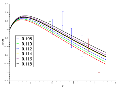
  Figure 1: Velocity drift (cm/sec/yr) versus redshift for inverse power law potential with different values of $K$ ($\gamma$ is fixed at 0.001). The bold black curve correspond to the $\Lambda CDM$ model.

• Exponential potential: This potential has the following form

  $$V(\phi)\,=\,V_{0}\,exp(-\phi/f)$$ (16)

  where $V_{0}$ and $f$ are positive constants [15, 16]. The exponential potential has the capability of producing scaling solutions which further scales the background energy density. But it require fine tuning of parameters to produce the late time acceleration. The corresponding Hubble parameter in this model is

  $$Y^{2}=\frac{X^{2}}{{6\beta}}+\frac{8\pi}{3}e^{-Z}+\Omega_{m}$$ (17)

  where $\beta=m_{pl}^{2}/(8\pi f^{2})$. The dimensionless variables are defined as:

  $$X=\frac{1}{{H_{0}f}}{\dot{\phi}},\;Y=\frac{H}{H_{0}},\;Z=\frac{\phi}{f}-\ln\left[\frac{V_{0}}{{m_{pl}^{2}H_{0}^{2}}}\right].$$

  Field equations can now be written as

  $$\frac{dX}{dz} = \frac{1}{(1+z)}\left[3X-8\pi\beta\frac{e^{-Z}}{Y}\right]$$

  $$\frac{dY}{dz} = \frac{1}{(1+z)}\left[\frac{3}{2}Y+\frac{1}{4\beta}\frac{X^{2}}{Y}-4\pi\frac{e^{-Z}}{Y}\right]$$ (18)

  $$\frac{dZ}{dz} = -\frac{1}{(1+z)}\left[\frac{X}{Y}\right]$$

  We solve the above system for parameter values $H_{0}=1.67\times 10^{-33}h$ $eV$, $m_{pl}=1.2\times 10^{28}eV$ and $h=0.7$. For these values for given set of parameters we choose initial values (redshift , $z\sim 3000$) $Z_{i}=1.5,X_{i}=10^{-9}$. Now for different values of the parameter $\beta$, we generate initial data sets by choosing $Y_{i}$ in such a way that $Y=1$ at $z=0$.

  The variation of the velocity drift for exponential potential model are shown in Fig. 2. It is clear from the figure that after certain value of $\beta$, the universe remains in the decelerated phase.

  

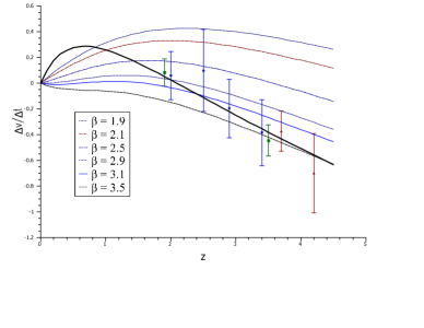
  Figure 2: Variation of velocity drift (cm/sec/yr) with redshift $z$ for $V=V_{0}exp(-\phi/f)$ . The bold black curve correspond to the $\Lambda CDM$ model.

• PNGB Model: In this (Pseudo-Nambu-Goldstone Bosons) model the scalar field potential has the following functional form

  $$V(\phi)\,=\,M^{4}\,\left(1+\,cos({\phi/f})\right)$$ (19)

  where $M$ and $f$ are positive constants [15, 17, 19]. The main motivation to study this potential is because of its special properties which not only explain late time acceleration but its ability to offer solution to the cosmic coincidence problem. The Hubble parameter for PNGB model in the term of dimensionless parameters is

  $$Y^{2}\,=\,\frac{4\pi}{3}\alpha^{2}\,X^{2}\,+\,1+\cos(Z)+\Omega_{m}$$ (20)

  where

  $$X=\frac{\dot{\phi}}{H_{0}f},\;Y=\frac{H}{H_{0}},\;Z=\frac{\phi}{f}$$ (21)

  and $\alpha=f/m_{pl}$. The full dynamical system in terms of variables $X,Y$ and $Z$ can be written analogues to earlier two cases as

  $$\frac{dX}{dz} = \frac{1}{(1+z)}\left[3X-\frac{m^{4}}{\alpha^{2}}\left(\frac{\sin Z}{Y}\right)\right]$$

  $$\frac{dY}{dz} = \frac{1}{(1+z)}\left[\frac{3}{2}Y+{2\pi\alpha^{2}}\frac{X^{2}}{Y}-{4\pi m^{4}}\left(\frac{1+\cos Z}{Y}\right)\right]$$

  $$\frac{dZ}{dz} = -\frac{1}{(1+z)}\left[\frac{X}{Y}\right].$$ (22)

  where $m^{4}=M^{4}/(m_{pl}H_{0})^{2}$. We choose initial values (redshift , $z\sim 3000$) $Z_{i}=1.5,X_{i}=10^{-9}$. Now for different values of the parameter $\alpha$, we generate initial data sets by choosing $Y_{i}$ in such a way that $Y=1$ at $z=0$.

  The variation of the velocity drift for PNGB model are shown in Fig. 3. It is clear from the figure that after a certain critical value of $\alpha$, universe always remain in the deceleration mode when the light is traveling toward us. For smaller values of $\alpha$, it shows the universe has undergone the decelerating phase twice.

  

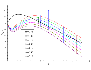
  Figure 3: Variation of velocity drift (cm/sec/yr) with redshift $z$ for $V=M^{4}(1+\cos(\phi/f))$ for $M=0.004{\sqrt{h}}\,eV$. The black curve correspond to the $\Lambda CDM$ model.

3.2 Modified Gravity Model

An important class of models which has attracted considerable attention in past few years is the one that modifies Einstein-Hilbert action by replacing Ricci tensor by an arbitrary function of curvature

$$S=\int\left(\frac{f(R)}{16\pi G}+{\cal L}_{m}\right)\sqrt{-g}\,d^{4}x.$$ (23)

In this letter we study the $f(R)$ theory model given recently by Starobinsky, Hu and Sawicki [20, 21] (see also, [22])

$$f(R)\,=\,R\,+\,\lambda R_{0}\left[\left(1\,+\,\frac{R^{2}}{R_{0}^{2}}\right)^{-n}\,\,-\,1\right]$$ (24)

where $\lambda$, $n$ and $R_{0}$ are positive parameters. For necessary steps leading to calculation of Hubble parameter see Dev et al. [23]. These models can evade local gravity constraints and have the capability being distinguished from the cosmological constant.

The Fig. 4 displays the variation of velocity drift for $f(R)$ model. There is very small difference between the variation of $H(z)$ with z for n =1 and n = 2 at the redshift $z\leq 1.8$ [23]. Hence for redshift $z\geq 1.8$, the variation of velocity drift becomes independent of the value of $n$.

Figure 4: Variation of velocity drift (cm/sec/yr) with redshift $z$ for $f(R)$ gravity model.

4 Results and Discussions

Till now, large number of theoretical models have been proposed to explain the observed accelerated expansion of the universe. In order to get insight of the mechanism behind this acceleration, we require complimentary observational tools. The observational tests either belong to distance based methods such as SNe Ia luminosity distances, angular size of compact radio sources, BAO, CMBR, gravitational lensing etc. or time based methods like Absolute age method, Lookback time method and Differential age method. Every observational tests requires some priors, assumptions and is subjected to systematic errors.

There is a need to develop tools which are simple and have a controlled systematics. The cosmological redshift drift (CRD) method is a test in this direction. Corasaniti et al. were the first to analyse dark energy models like $\Lambda$CDM, Chaplygin gas and dark energy- dark matter interaction model using the CRD test [24]. They conclude that the CRD test puts stringent constraints on non-standard dark energy models. Later on, Balbi and Quercellini also investigated various standard and non-standard dark energy models [25]. They found the worst bound for the Cardassian model. Further Zhang et al. also studied Holographic dark energy model with CRD test [26] and obtain a very tight bound on the $\Omega_{m}$. The above stated work used the data generated by MC simulations, given by Pasquini et al. (2006) [12].

Uzan, Bernardeau and Mellier discuss the possibility in which the large scale structure may effect the measurements of time drift of the cosmological redshift [27]. Since the CRD test is based on the assumption that the universe is homogeneous and isotropic, therefore this test has been used to check the homogeneity of the universe [28]. Quartin and Amendola propose that CRD test can be used to distinguish between Void models and conventional dark energy scenarios [29]. Recently one possible source of noise in the CRD test has been studied by Killedar and Lewis which deal with the transverse motion of the Ly$\alpha$ absorbers [30].

Recently Liske et al. (2008) studied in detail the impact of next generation ELT on observing the very small redshift drift signal [6]. Using the extensive MC simulations, three sets of data points are generated with different strategies which include the measurement of the precise value of velocity shift. In our work, We used the recent data generated by Liske at al.(2008) to constrain the late time acceleration models of the universe. We study the models which belong to both the Einstein gravity scenario ($\Lambda$CDM, XCDM, scalar field potentials) and the modified gravity ($f(R)$).

Results are summarized as follows:

1. In $\Lambda$CDM model $(w_{x}=-1)$, the $\chi^{2}$ minimum lies at $\Omega_{m0}=0.3$. Considering $h$ to be a nuisance parameter, we marginalize over $h$ to obtain the probability distribution function defined as:

   $$L(p)\,=\,\int{e^{-\chi^{2}(h,p)/2}P(h)dh}$$

   Here P(h) is the prior probability function for $h$ which is assumed to be Gaussian. We find that the best fit value of model parameter is independent of the choice of prior.

2. We performed the $\chi^{2}$ statistics on flat XCDM dark energy model as shown in Fig. 5. The best fit values lies at $\Omega_{m}=0.3$ and $w_{x}=-1$. At $1\sigma$-level the constraints are,

   $$\Omega_{m}\,=\,0.30^{+0.03}_{-0.04}\hskip 56.9055pt\omega_{x}\leq-0.62$$

   Here again we marginalize over $h$ to obtain the best fit value of model parameters $(\Omega_{m},w_{x})$. The best fit values are independent of the choice of prior. The redshift drift test give very tight constraint on the $\Omega_{m}$ and weak bound on the equation of state, $\omega_{x}$. This is expected since the amplitude and slope of the cosmic velocity shift w.r.t the redshift is very sensitive to the $\Omega_{m}$ and shows weak dependence on the equation of state. The other important feature of this analysis is that it is complementary to other probes such as CMB, BAO and weak lensing.

   

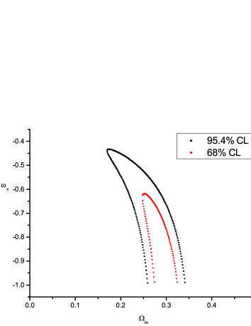
   Figure 5: Flat dark energy model with constant $\omega_{x}$: Contours in $\Omega_{m}$ and $\omega_{x}$ plane for CRD test. The best fit value lies at $\Omega_{m}=0.3$ and $\omega_{x}=-1$. The inner and outer curves are at $1\sigma$ and $2\sigma$ respectively.

3. We analyze the $f(R)$ gravity model proposed by Starobinsky with the CRD test. The variation of velocity drift for different values of $n$ with redshift $z$ is shown in Fig. 4. The expansion history of this model match exactly with the $\Lambda$CDM model for $n=2$ and $\lambda=2$. In this model the Hubble parameter, $H(z)$, becomes independent of the parameter $n$ after the redshift $z=1.8$ and expansion history traces exactly the $\Lambda$CDM model behavior at high redshift [31, 23]. Since the simulated data points have $z\geq 1.9$, the $\chi^{2}$ for this model will be the same as for the $\Lambda$CDM model. Here $\Lambda$CDM model means standard cosmological model with $\omega_{x}=-1$, $\Omega_{m0}=0.3$ and $\Omega_{\Lambda 0}=0.7$ . The effective equation of state for this model appproaches $\omega=-1$ at the present epoch [see Fig.8 of the ref.[23]]. In order to constrain this model better we need redshift drift data in the redshift range $z\leq 1.9$ .

4. In Fig. 6, we plot the variation of $\chi^{2}$ with the parameter $\beta$ for the exponential potential. The best fit value of $\beta=m_{pl}^{2}/(8\pi f^{2})=3.2$ corresponds to $\Omega_{m0}=0.26$. The $\chi^{2}$ per degree of freedom is 0.67. At $3\sigma$ limit, the allowed range of $\beta=3.2^{-0.45}_{+0.55}$ gives $\Omega_{m}=0.26^{-0.05}_{+0.06}$. Although the model predicts the observed value of $\Omega_{m}$ but still this model is not fully in concordance with the observations; as the allowed range of $\beta$ at $3\sigma$ level shows that the universe mostly remains in a decelerating phase (see Fig. 2).

   

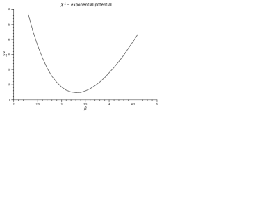
   Figure 6: Variation of $\chi^{2}$ with $\beta$

5. In the inverse power law potential model, for $\gamma\rightarrow 0$, the energy-momentum tensor approaches towards cosmological constant. The best fit values for this model are $\gamma=0.025$ and $K=0.118$. In Fig. 7 the contour is plotted in $\gamma-K$ plane. We would like to note here that computational efforts to generate the data points in the neighborhood of $\gamma=0$ increases. The important feature of this contour is that it is complementary to the contour obtain by using the Dark Energy Task Force (DETF) simulated data sets for future experiments. This includes SNe Ia, BAO, weak Lensing and CMB (PLANCK) observations [32].

   In the Fig. 8 variation of instantaneous equation of state is plotted w.r.t. redshift for the best fit values of the model parameters. There is almost no variation in the equation of state with redshift. It always stay close to $\omega=-1$ for the redshift range studied here.

   

   Figure 7: Contour in $\gamma-K$ plane for inverse power law potential. The inner and the outer contours are drawn at the 1$\sigma$ and 2$\sigma$ level respectively.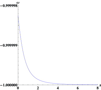

   

   Figure 8: Variation of $\omega$ w.r.t. redshift for inverse power law potential.

6. For the PNGB model, the contour is plotted in $\alpha-m$ plane as shown in the Fig. 9. The $\chi^{2}$ minimum lies at $\alpha=0.21$ for $m=0.56$. At 2$\sigma$ level, $\alpha>0.15$ is allowed. This result is completely in concordance with the other cosmological observations (eg. SNe Ia, lensing, cluster observations) [15, 17, 18]. Again this contour is complementary to the contour obtain by using Markov Chain Monte Carlo analysis (MCMC) to generate the future data set. This includes future SNe Ia, BAO, weak Lensing and cosmic microwave background observations [33].

   In the Fig. 10 instantaneous equation of state is plotted for the best fit values. In contrast to power law potential, the PNGB show large variation in equation of state for the redshift $z<2$.

   

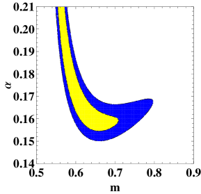
   Figure 9: Contour in $\alpha-m$ plane for PNGB potential. The inner and the outer contours are drawn at the 1$\sigma$ and 2$\sigma$ level respectively.

   

   Figure 10: Variation of $\omega$ w.r.t. redshift for for PNGB potential.

   It is clear that CRD test is a very simple, straightforward and powerful tool which probes the expansion history of the universe directly. In future the precision data especially in redshift range of $z<2$ shall add to the predictive power of CRD test.

References

- [1] T. Padmanabhan, Phys. Rept., 380 (2003) 235; E. J. Copeland, M. Sami & S. Tsujikawa, Int. J. Mod. Phys., D15 (2006) 1753; V. Sahni, A. Starobinsky, Int. J. Mod. Phys., D15 (2006) 2105; J. S. Alcaniz, Braz. J. Phys, 36 (2006) 1109; J. A. Frieman, M. Turner & D. Huterer, Ann. Rev. Astron. Astrophys., 46 (2008) 385; R. R. Caldwell & M. Kamionkowski, [arXiv:0903.0866]; J. P. Uzan, [arXiv:0908.2243]
- [2] E. V. Linder, Rep. Prog. Phys., 71 (2008) 056901.
- [3] J. Nordin, A. Goobar & J. Jonsson, JCAP 0802 (2008) 008.
- [4] D. Huterer & M. S. Turner, Phys. Rev. D., 64 (2001) 123527 ; E. V. Linder, Phys. Rev. D., 72 (2005) 043529; E. V. Linder & R. N. Cahn, Astropart. Phys., 28 (2007) 481.
- [5] V. D’Odorico, et al., [arXiv:0708.1258].
- [6] J. Liske et al., Mon. Not. Roy. Astr. Soc., 386 (2008) 1192.
- [7] A. Sandage, Astrophys. J., 136 (1962) 319.
- [8] G. C. McVittie, Astrophys. J., 136 (1962) 334; S. Weinberg, Gravitation and Cosmology, (New York: Wiley, 1972); R. Rudiger, Astrophys. J., 240 (1980) 384; K. Lake, Astrophys. J., 247 (1981) 17; R. Rudiger, Astrophys. J., 260 (1982) 33; E. V. Linder, First Principles of Cosmology, 1997 (London: Addison - Wesley); K. Lake, Phys. Rev. D., 76 (2007) 063508.
- [9] A. Loeb, Astrophys. J., 499 (1998) L111.
- [10] G. C. McVittie , Astrophys. J., 136 (1962) 334.
- [11] L. Pasquini et al., IAU symposium, ed. P. Whitelock , M. Dennefeld & B. Leibundgut, 232 (2006) 193.
- [12] L. Pasquini et al., The Messenger, 122 (2005) 10.
- [13] J. Liske et al., The Messenger, 133 (2008) 10; J. Liske, et al., [arXiv:0802.1926]; S. Cristiani, [arXiv: 0712.4152]
- [14] P. J. E. Peebles & B. Ratra, Astrophys. J., 325 (1998) L17; B. Ratra, & P. J. E. Peebles, Phys. Rev. D., 37 (1998) 3406.
- [15] J. A. Frieman & I. Waga, Phys. Rev. D., 57 (1998) 4642.
- [16] V. Sahni, H. Feldman & A. Stebbins, Astrophys. J., 385 (1992) 1; C. Wetterich, Astron. Astrphys., 301 (1995) 321; E. J. Copeland, A. R. Liddle & D. Wands, Phys. Rev. D., 57 (1998) 4686; P. G. Ferreira & M. Joyce, Phys. Rev. D., 58 (1998) 023503.
- [17] S. C. Cindy Ng & D. L. Wiltshire , Phys. Rev. D., 64 (2001) 123519.
- [18] I. Waga & J. A. Frieman, Phys. Rev. D., 62 (2000) 043521.
- [19] J. A. Frieman et al., Phys. Rev. Lett., 75 (1995) 2077.
- [20] A. A. Starobinsky, JETP Lett., 86 (2007) 157.
- [21] W. Hu & I. Sawicki , Phys. Rev. D., 76 (2007) 064004.
- [22] A. V. Frolov, Phys. Rev. Lett., 101 (2008) 061103.
- [23] A. Dev, D. Jain, S. Jhingan, S. Nojiri, M. Sami & I. Thongkool, Phys. Rev. D., 78 (2008) 083515.
- [24] P. S. Corasaniti, D. Huterer & A. Melchiorri, Phys. Rev. D., 75 (2007) 062001.
- [25] A. Balbi & C. Quercellini, Mon. Not. Roy. Astr. Soc., 382 (2007) 1623.
- [26] H. Zhang et al., Phys. Rev. D., 76 (2007) 123508.
- [27] J. P. Uzan, F. Bernardeau & Y. Mellier, Phys. Rev. D., 77 (2008) 021301.
- [28] J. P. Uzan, C. Clarkson & G. F. R. Ellis , Phys. Rev. Lett., 100 (2008) 191303; D. L. Wiltshire, Phys. Rev. D., 80 (2009) 123512.
- [29] M. Quartin & L. Amendola, [arXiv:0909.4954].
- [30] M. Killedar & G. F. Lewis , [arxiv:0910.4580].
- [31] S. Nojiri & S. D. Odintsov, Phys. Rev. D., 74 (2006) 086005; S. Nojiri & S. D. Odintsov, Phys. Letts. B, 657 (2007) 238.
- [32] M. Yashar et al.,Phys. Rev. D., 79 (2009) 103004.
- [33] A. Abrahamse et al.,Phys. Rev. D., 77 (2008) 103503.