Superconductivity in the doped bilayer Hubbard model.

Abstract

We study by the Gutzwiller approximation the melting of the valence bond crystal phase of a bilayer Hubbard model at sufficiently large inter-layer hopping. We find that a superconducting domain, with order parameter $d_{z^{2}-r^{2}}$, $z$ being the inter-layer direction and $r$ the intra-layer one, is stabilized variationally close to the half-filled non-magnetic Mott insulator. Superconductivity exists at half-filling just at the border of the Mott transition and extends away from half-filling into a whole region till a critical doping, beyond which it gives way to a normal metal phase. This result suggests that superconductivity should be unavoidably met by liquefying a valence bond crystal, at least when each layer is an infinite coordination lattice and the Gutzwiller approximation becomes exact. Remarkably, this same behavior is well established in the other extreme of two-leg Hubbard ladders, showing it might be of quite general validity.

I Introduction

Since its original formulation in the early 60th’s, the Gutzwiller variational approach Gutzwiller (1963, 1964, 1965) has proved to be one of the simplest yet effective tools to deal with correlated electron systems.

The basic idea of the method is to modify variationally the weights of local electronic configurations with respect to an uncorrelated wavefunction $|\Psi_{0}\rangle$, for which Wick’s theorem holds, according to the local interaction terms. This is accomplished by means of the variational wavefunction:

$$|\Psi_{G}\rangle=\mathcal{P}|\Psi_{0}\rangle=\prod_{\mathbf{R}}\,\mathcal{P}_{\mathbf{R}}\,|\Psi_{0}\rangle,$$ (1)

where $\mathcal{P}_{\mathbf{R}}$ is an operator acting on the local Hilbert space of the unit cell $\mathbf{R}$. Both the uncorrelated wavefunction $|\Psi_{0}\rangle$ and the operators $\mathcal{P}_{\mathbf{R}}$ must be determined variationally by minimizing the average energy. In general the average energy can be calculated only numerically Sorella (2005) but in the limit of infinite coordination lattices, where a lot of simplifications intervene Müller-Hartmann (1989) that allow for an explicit analytical expression Metzner and Vollhardt (1987, 1988); Bünemann et al. (1998). This is rigorously valid only in infinite coordination lattices, nevertheless it is commonly used also in finite coordination ones, what is refereed to as the Gutzwiller approximation because in a single band model it happens to coincide with the approximation introduced by Gutzwiller himself Gutzwiller (1965).

In spite of its simplicity, many important concepts in strongly correlated electron systems have originated from Gutzwiller variational calculations or, which is equivalent Kotliar and Ruckenstein (1986); Bunemann and Gebhard (2007), from slave-boson mean-field theory Kotliar and Ruckenstein (1986); Lechermann et al. (2007). We just mention the famous Brinkmann-Rice scenario Brinkman and Rice (1970) of the Mott transition. Therefore, even though more rigorous approaches have been developed meanwhile, like DMFT Georges et al. (1996) or LDA+U Anisimov et al. (1997), there has been a continuous effort towards improving the original Gutzwiller wavefunction in finite dimensions Capello et al. (2005), and extending the Gutzwiller approximation to account for the exchange interaction in multi-orbital models Bünemann et al. (1998, 2005); Attaccalite and Fabrizio (2003); Fabrizio (2007), for the electron-phonon coupling Barone et al. (2007), for interfaces effects Borghi et al. (2009), and also for more ab-initio ingredients Deng et al. (2009). A reason for this perseverance is that the Gutzwiller wavefunction and approximation are so simple and flexible to be adapted to many different situations and provide without big numerical efforts reasonable results.

In its simplest formulation, Eq. (1), the form of intersite correlations within the Gutzwiller wavefunction are controlled solely by the uncorrelated wavefunction $|\Psi_{0}\rangle$. This aspect should not be problematic if the main interest is in the gross features near a Mott transition or when a Hartree-Fock Slater determinant gives already a reasonable description of the actual ground state, which can only be improved by applying the operator $\mathcal{P}$. However, there are interesting cases where new types of correlations may arise near a Mott transition that are not explicitly present in the Hamiltonian. A known example are the $d$-wave superconducting fluctuations that are believed to emerge in the single band Hubbard model on a square lattice close to the half-filled antiferromagnetic Mott insulator Bickers et al. (1989), and which are often invoked to explain high T_c superconductivity. A simple way to justify the emergence of superconducting fluctuations is to take the large $U$ limit of the Hubbard model, which is known to correspond in the low energy sector to the $t$-$J$ model. Here, the antiferromagnetic exchange $J$ provides an explicit attraction in the inter-site singlet channel. This reflects the tendency of neighboring sites to form spin singlets, which turns into a true antiferromagnetic long-range order at half-filling but may mediate superconductivity upon doping. Indeed, the Gutzwiller approximation and equivalently the slave-boson mean-field theory applied to the $t$-$J$ model do stabilize a $d$-wave superconducting phase away from half-filling Kotliar and Liu (1988), a result supported by direct numerical optimizations of $|\Psi_{G}\rangle$, with $\mathcal{P}_{\mathbf{R}}$ projecting out doubly occupied sites and $|\Psi_{0}\rangle$ a $d$-wave BCS-like wavefunction Gros (1988); Paramekanti et al. (2004); Sorella et al. (2002); Anderson et al. (2004). However, the simplest Gutzwiller approximation in the pure Hubbard model away from half-filling does not stabilize any superconducting phase, just because the on-site repulsion $U$ does not couple directly to the $d$-wave superconducting parameter. A way to improve the wavefunction allowing for inter-site spin-singlet correlations could be using an enlarged non-primitive unit cell, with $\mathcal{P}_{\mathbf{R}}$ in (1) acting on a cluster of sites. With this choice the wavefunction $|\Psi_{G}\rangle$ breaks explicitly lattice translational symmetry, so that one should properly modify the variational scheme not to get spurious results, just like any other cluster technique Lichtenstein and Katsnelson (2000); Potthoff et al. (2003); Senechal et al. (2000); Kotliar et al. (2001); Maier et al. (2005); Dahnken et al. (2004).

Alternatively, one might consider different models that are manageable with the simple wavefunction (1) and which are expected to have a physical behavior similar to the one looked for in the Hubbard model on a square lattice. One case by now well known is that of two coupled Hubbard or $t$-$J$ chains. At half-filling, both models are non-magnetic Mott insulators Strong and Millis (1994); Shelton et al. (1996); Balents and Fisher (1996). The insulating phase is a kind of short-range resonating valence bond (RVB) spin-liquid Sierra et al. (1998), i.e. a spin-gaped state without any symmetry breaking. Actually this state is adiabatically connected to the trivial insulator for very large inter-chain coupling, which is a collection of inter-chain dimers, what can be denoted as a valence bond (VB) crystal. Away from half-filling, dominant superconducting fluctuations arise Fabrizio (1993); Balents and Fisher (1996); Schulz (1999), with a two-chain analog of a two-dimensional $d$-wave symmetry. The emergence of strong superconducting fluctuations appears here as the natural fate of doping the half-filled VB Mott insulator Sierra et al. (1998), realizing in one-dimension the RVB superconductivity scenario proposed by Anderson Anderson (1987) in the early days after the discovery of high T_c superconductivity. An immediate question that arises is whether the above one-dimensional behavior survives in higher-dimensions, namely how robust is the two-chain RVB scenario upon increasing dimensionality. This is actually the content of the present work.

As a matter of fact, this question has been already addressed several times in connection with high T_c superconductors, specifically analyzing a bilayer Hubbard model by various techniques, including quantum Monte Carlo Sandvik and Scalapino (1994); Scalettar et al. (1994); dos Santos (1995); Wang et al. (2006); Bouadim et al. (2008) (QMC) and DMFT Fuhrmann et al. (2006); Kancharla and Okamoto (2007). In section II we shall discuss more in detail these early works while introducing the model. More recently, the same problem has been studied at half-filling by an improved Gutzwiller approximation Fabrizio (2007), which we present in section III together with a further improvement that we use here to extend that analysis away from half-filling. The results are presented in section IV, while section V is devoted to concluding remarks.

II The model

Throughout this work we shall be interested in a bilayer Hubbard model described by the following Hamiltonian

$$\mathcal{H} = -\sum_{\mathbf{R}\mathbf{R^{\prime}}}\,\sum_{i=1}^{2}\,\sum_{\sigma}\,t_{\mathbf{R}\mathbf{R^{\prime}}}\,c^{\dagger}_{\mathbf{R},i\sigma}c^{\phantom{\dagger}}_{\mathbf{R^{\prime}},i\sigma}+H.c.$$ (2)

$$+\frac{U}{2}\sum_{\mathbf{R}}\,\sum_{i=1}^{2}\,(n_{\mathbf{R},i}-1)^{2}$$

$$-t_{\perp}\,\sum_{\mathbf{R}}\,\sum_{\sigma}\,\left(c^{\dagger}_{\mathbf{R},1\sigma}c^{\phantom{\dagger}}_{\mathbf{R},2\sigma}+H.c.\right)$$

$$= \sum_{\mathbf{k}\sigma}\,\sum_{i=1}^{2}\,\epsilon(\mathbf{k})\,c^{\dagger}_{\mathbf{k},i\sigma}c^{\phantom{\dagger}}_{\mathbf{k},i\sigma}$$

$$+\frac{U}{2}\sum_{\mathbf{R}}\,\sum_{i=1}^{2}\,(n_{\mathbf{R},i}-1)^{2}$$

$$-t_{\perp}\,\sum_{\mathbf{k}\sigma}\,\left(c^{\dagger}_{\mathbf{k},1\sigma}c^{\phantom{\dagger}}_{\mathbf{k},2\sigma}+H.c.\right)$$

$$\equiv\mathcal{H}_{hop}+\mathcal{H}_{U}+\mathcal{H}_{\perp},$$

where $t_{\perp}>0$, $c^{\dagger}_{\mathbf{R},i\sigma}$ and $c^{\phantom{\dagger}}_{\mathbf{R},i\sigma}$ create and annihilate, respectively, an electron at site $\mathbf{R}$ in plane $i=1,2$ with spin $\sigma$, $n_{\mathbf{R},i}=\sum_{\sigma}\,c^{\dagger}_{\mathbf{R},i\sigma}c^{\phantom{\dagger}}_{\mathbf{R},i\sigma}$ is the local occupation on layer $i$, and $U$ is the Hubbard repulsion on each lattice site. In order to study the doped system it is more convenient to work in the grand-canonical ensemble adding a chemical potential term $-\mu\sum_{\mathbf{R},i}n_{\mathbf{R},i}$ to the model Hamiltonian (2). The particle number is then controlled by tuning $\mu$. In Eq. (2) $c^{\dagger}_{\mathbf{k},i\sigma}$ creates an electron in layer $i$ and spin $\sigma$ with momentum $\mathbf{k}$, and $\epsilon(\mathbf{k})\in[-D,D]$ is the intra-layer dispersion in momentum space, where $D$ is half the bandwidth that will be our unit of energy. The non-interacting part of the Hamiltonian is better rewritten introducing the bonding ($e$) and antibonding ($o$) combinations

$$c^{\dagger}_{\mathbf{k},e\sigma} = \frac{\displaystyle 1}{\displaystyle\sqrt{2}}\left(c^{\dagger}_{\mathbf{k},1\sigma}+c^{\dagger}_{\mathbf{k},2\sigma}\right),$$

$$c^{\dagger}_{\mathbf{k},o\sigma} = \frac{\displaystyle 1}{\displaystyle\sqrt{2}}\left(c^{\dagger}_{\mathbf{k},1\sigma}-c^{\dagger}_{\mathbf{k},2\sigma}\right),$$

through which

$$\mathcal{H}_{hop}+\mathcal{H}_{\perp}=\sum_{\mathbf{k}\sigma}\,\sum_{a=e,o}\,\epsilon_{a}(\mathbf{k})\,c^{\dagger}_{\mathbf{k},a\sigma}c^{\phantom{\dagger}}_{\mathbf{k},a\sigma},$$ (3)

where $\epsilon_{e}(\mathbf{k})=\epsilon(\mathbf{k})-t_{\perp}\in\left[-D-t_{\perp},D-t_{\perp}\right]$ and $\epsilon_{o}(\mathbf{k})=\epsilon(\mathbf{k})+t_{\perp}\in\left[-D+t_{\perp},D+t_{\perp}\right]$ are, respectively, the bonding and antibonding band dispersions.

If $U=0$ and the density is one electron per site, half-filling, the model describes a metal until the two bands overlap, i.e. $t_{\perp}\leq D$, and a band insulator otherwise.

For $U\gg D+t_{\perp}$, the model becomes equivalent to two Heisenberg planes coupled to each other by an inter-plane antiferromagnetic exchange $J_{\perp}=4t_{\perp}^{2}/U$. If each plane is a square lattice with only nearest neighbor hopping $t$, hence $D=4t$, each Heisenberg model is characterized by a nearest neighbor antiferromagnetic exchange $J=4t^{2}/U$. This model has been studied in detail by quantum Monte Carlo Sandvik and Scalapino (1994); Wang et al. (2006) and it is known to have a quantum critical point that separates a a Neèl antiferromagnet, for $J_{\perp}\leq 2.5520\,J$, from a gaped spin-liquid phase, for larger $J_{\perp}$. The latter can be interpreted as a kind of VB crystal, each bond being an inter-layer singlet, adiabatically connected to the band insulator at $U=0$. In terms of the hopping parameters of the original Hubbard bilayer, the critical point should correspond to $(t_{\perp}/t)_{c}=\sqrt{2.5220}\simeq 1.5881$. This value is in good agreement with direct QMC simulations of the Hubbard bilayer Scalettar et al. (1994); Bouadim et al. (2008), which find $(t_{\perp}/t)_{c}\simeq 1.5$ to 2. According to these results, when $1.6\leq(t_{\perp}/t)\leq 4$ one could start at $U=0$ with a metallic phase, and, upon increasing $U$, find a direct transition into the VB Mott insulator. However, the story must become more complicated if the $U=0$ Fermi surface at half-filling has nesting at the edge of the Brillouin zone, as it happens for a square lattice with only nearest neighbor hopping. In this case, the $U=0$ and $t_{\perp}<4t=D$ metal has a Stoner instability towards Neèl antiferromagnetism for arbitrary small $U$, so that it is a priori not obvious that one could find any direct metal to VB Mott insulator transition. In reality, both cluster DMFT Kancharla and Okamoto (2007) and QMC simulations find evidence that such a transition does exist. Nevertheless, one may always bypass this problem assuming that the intra-layer hopping is such as not to lead to any nesting, the latter being more an accident than the rule in realistic systems. In this case, which we will implicitly assume hereafter, it is safe to believe that a direct transition at half-filling from a metal to a VB Mott insulator does exist.

Within this scenario, the melting of the VB crystal into a metallic phase can therefore occur either by doping away from half-filling but also upon decreasing $U$ below the Mott transition, still keeping half-filled density. In the latter case, a recent study Fabrizio (2007) has shown that, within the Gutzwiller approximation, the VB crystal first turns into a superconducting phase that eventually gives way to a normal metal upon further decreasing $U$. This finding supports the RVB superconductivity scenario Anderson (1987) and shows that the one-dimensional behavior persists in higher dimensions. It also agrees with the indication of an enhanced pairing susceptibility obtained in earlier studies by QMC Bulut et al. (1992); dos Santos (1995). However the lowest temperatures attainable so far by QMC are still above the eventual superconducting critical temperature, so that the existence of a true superconducting phase at half-filling is numerically still an open issue. DMFT calculations, that could in principle be carried out at zero temperature, was performed Fuhrmann et al. (2006); Kancharla and Okamoto (2007) but did not search explicitly for any superconducting phase.

Away from half-filling, QMC indications of enhanced pairing fluctuations are more convincing dos Santos (1995); Bouadim et al. (2008), although the existence of a superconducting phase at low temperature is still uncertain dos Santos (1995). This makes it worth addressing this issue by the Gutzwiller approximation, which is not as rigorous as QMC but at least can provide results at zero temperature.

III The method

In order to study the bilayer Hubbard model (2) away from half-filling we adopt the Gutzwiller approximation scheme developed in Refs. Fabrizio, 2007 to deal with the same model at half-filling. The variational wavefunction that we use has the form as in Eq. (1) where

• $\mathcal{P}_{\mathbf{R}}$ acts on the full Hilbert space that includes site $\mathbf{R}$ in layer 1 and site $\mathbf{R}$ in layer 2;

• $|\Psi_{0}\rangle$ is allowed to be a BCS-wavefunction with singlet order parameter in the channel $c^{\dagger}_{\mathbf{R},1\uparrow}c^{\dagger}_{\mathbf{R},2\downarrow}+c^{\dagger}_{\mathbf{R},2\uparrow}c^{\dagger}_{\mathbf{R},1\downarrow}$.

The most general expression for $\mathcal{P}_{\mathbf{R}}$ is:

$$\mathcal{P}_{\mathbf{R}}=\sum_{\Gamma_{1},\Gamma_{2}}\,\lambda(\mathbf{R})_{\Gamma_{1}\Gamma_{2}}\,|\Gamma_{1},\mathbf{R}\rangle\langle\Gamma_{2},\mathbf{R}|,$$ (4)

where each state $|\Gamma_{i},\mathbf{R}\rangle$ denotes a local two-site electronic configuration, and the matrix $\lambda(\mathbf{R})$ has to be variationally determined. Average values of operators on the wavefunction (1) can be analytically computed in infinite-coordination lattices provided the following constraints are satisfied by $\mathcal{P}_{\mathbf{R}}$ Bünemann et al. (1998); Attaccalite and Fabrizio (2003); Fabrizio (2007):

$$\langle\Psi_{0}|\,\mathcal{P}^{\dagger}_{\mathbf{R}}\,\mathcal{P}^{\phantom{\dagger}}_{\mathbf{R}}\,|\Psi_{0}\rangle = 1,$$ (5)

$$\langle\Psi_{0}|\,\mathcal{P}^{\dagger}_{\mathbf{R}}\,\mathcal{P}^{\phantom{\dagger}}_{\mathbf{R}}\,\mathcal{C}_{\mathbf{R}}\,|\Psi_{0}\rangle = \langle\Psi_{0}|\,\mathcal{C}_{\mathbf{R}}\,|\Psi_{0}\rangle,$$ (6)

where $\mathcal{C}_{\mathbf{R}}$ is the local single-particle density-matrix operator with elements $c^{\dagger}_{\mathbf{R},\alpha}c^{\phantom{\dagger}}_{\mathbf{R},\beta}$ and $c^{\dagger}_{\mathbf{R},\alpha}c^{\dagger}_{\mathbf{R},\beta}$, $\alpha$ and $\beta$ labeling single-particle states (both layer and spin indices) and $c^{\dagger}_{\mathbf{R},\alpha}$($c^{\phantom{\dagger}}_{\mathbf{R},\alpha}$) creating(annihilating) an electron in state $\alpha$ at site $\mathbf{R}$. Expectation values of local operators are then computed straightforwardly Fabrizio (2007) as $\langle\,\mathcal{P}^{\dagger}\mathcal{O}_{\mathbf{R}}\mathcal{P}\,\rangle_{0}=\langle\,\mathcal{P}^{\dagger}_{\mathbf{R}}\mathcal{O}_{\mathbf{R}}\mathcal{P}_{\mathbf{R}}\,\rangle_{0}$ (hereafter $\langle\,...\,\rangle_{0}$ denotes averages on the uncorrelated wavefunction $|\Psi_{0}\rangle$, which can be easily computed by means of Wick’s theorem). When calculating the average of the inter-site density matrix, one finds that the physical single-fermion operator acting on $|\Psi_{G}\rangle$ is effectively replaced by a renormalized one acting on $|\Psi_{0}\rangle$ according to:

$$c^{\dagger}_{\mathbf{R},\alpha}\rightarrow\sum_{\beta}R(\mathbf{R})_{\alpha\beta}\,c^{\dagger}_{\mathbf{R},\beta}+\sum_{\beta}Q(\mathbf{R})_{\alpha\beta}\,c^{\phantom{\dagger}}_{\mathbf{R},\beta},$$ (7)

where the renormalization matrices $R$ and $Q$ are determined by inverting the following set of equationsFabrizio (2007):

$$\langle\,\mathcal{P}^{\dagger}_{\mathbf{R}}c^{\dagger}_{\mathbf{R},\alpha}\mathcal{P}_{\mathbf{R}}c^{\phantom{\dagger}}_{\mathbf{R},\beta}\,\rangle_{0}=\sum_{\gamma}\,R(\mathbf{R})_{\alpha\gamma}\,\langle\,c^{\dagger}_{\mathbf{R},\gamma}c^{\phantom{\dagger}}_{\mathbf{R},\beta}\,\rangle_{0}$$

$$~{}~{}~{}~{}~{}~{}~{}~{}~{}+\sum_{\gamma}\,Q(\mathbf{R})_{\alpha\gamma}\,\langle\,c^{\phantom{\dagger}}_{\mathbf{R},\gamma}c^{\phantom{\dagger}}_{\mathbf{R},\beta}\,\rangle_{0},$$ (8)

$$\langle\,\mathcal{P}^{\dagger}_{\mathbf{R}}c^{\dagger}_{\mathbf{R},\alpha}\mathcal{P}_{\mathbf{R}}c^{\dagger}_{\mathbf{R},\beta}\,\rangle_{0}=\sum_{\gamma}\,R(\mathbf{R})_{\alpha\gamma}\,\langle\,c^{\dagger}_{\mathbf{R},\gamma}c^{\dagger}_{\mathbf{R},\beta}\,\rangle_{0}$$

$$~{}~{}~{}~{}~{}~{}~{}~{}~{}+\sum_{\gamma}\,Q(\mathbf{R})_{\alpha\gamma}\,\langle\,c^{\phantom{\dagger}}_{\mathbf{R},\gamma}c^{\dagger}_{\mathbf{R},\beta}\,\rangle_{0}.$$ (9)

In Ref. Fabrizio, 2007, a different notation was used for the matrices $R$ and $Q$, namely $R=\sqrt{Z}$ and $Q=\sqrt{\Delta}$. In order not to generate any confusion with the definition of a square root of a matrix, and also for keeping more explicit the connection with slave-boson mean field theory Lechermann et al. (2007), we have preferred here to use $R$ and $Q$. Despite the considerable simplification introduced by the infinite-coordination limit, the variational problem remains still a difficult task to deal with because of the large size of the local Hilbert space, which contains 16 states so that $\lambda$ spans in principle $16\times 16$ matrices.

A further simplification can be achieved with a proper choice of the basis set spanning the local Hilbert space. This can be done, for instance, by using from the beginning the natural basis, i.e., the single-particle basis which diagonalizes the variational density matrix $\langle\,\mathcal{C}_{\mathbf{R}}\,\rangle_{0}$Fabrizio (2007). An alternative and more efficient approach consistsLanatà et al. (2008) in defining the local operator $\mathcal{P}_{\mathbf{R}}$ in a mixed-basis representation, namely expressing $|\Gamma_{1},\mathbf{R}\rangle=|\Gamma,\mathbf{R}\rangle$ in Eq. (4) in the original basis defined by the model Hamiltonian and assuming that $\langle\Gamma_{2},\mathbf{R}|=\langle\{\bar{n}_{\alpha}\},\mathbf{R}|$ are Fock states in the natural basis, identified by the occupation numbers $\bar{n}_{\alpha}=0,1$. With this choice, one can use as variational parameters just the eigenvalues of the density matrix, because the unitary transformation that relates the natural-basis operators $d^{\phantom{\dagger}}_{\mathbf{R},\alpha}$ to the original ones $c^{\phantom{\dagger}}_{\mathbf{R},\alpha}$ needs not to be known explicitly. This simplifies considerably all calculations. In the mixed original-natural basis representation one introduces a new matrix

$$\phi(\mathbf{R})=\lambda(\mathbf{R})\,\sqrt{P^{0}(\mathbf{R})},$$ (10)

where $\lambda(\mathbf{R})$ is the variational matrix in the mixed-basis representation and $P^{0}(\mathbf{R})$ is the uncorrelated occupation-probability matrix, with elements

$$P^{0}_{\{\bar{n}_{\alpha}\},\{\bar{m}_{\alpha}\}}(\mathbf{R})\equiv \langle\,|\{\bar{m}_{\alpha}\},\mathbf{R}\rangle\langle\{\bar{n}_{\alpha}\},\mathbf{R}|\,\rangle_{0}$$

$$=\delta_{\{\bar{n}_{\alpha}\}\{\bar{m}_{\alpha}\}}\,P^{0}_{\{\bar{n}_{\alpha}\}}(\mathbf{R}),$$

being

$$P^{0}(\mathbf{R})_{\{\bar{n}_{\alpha}\}}=\prod_{\alpha}\,\left(n^{0}(\mathbf{R})_{\alpha}\right)^{\bar{n}_{\alpha}}\,\left(1-n^{0}(\mathbf{R})_{\alpha}\right)^{1-\bar{n}_{\alpha}},$$ (11)

and $n^{0}(\mathbf{R})_{\alpha}$ the eigenvalues of the density matrix (to be variationally determined). In terms of $\phi$, the constraints to be imposed on the Gutzwiller wavefunction can be recast asLanatà et al. (2008):

$$\mathrm{Tr}\left(\phi^{\dagger}\phi\right) = 1,$$ (12)

$$\mathrm{Tr}\left(\phi^{\dagger}\phi\,d^{\dagger}_{\alpha}d^{\phantom{\dagger}}_{\beta}\right) = \delta_{\alpha,\beta}\,n^{0}_{\alpha},$$ (13)

$$\mathrm{Tr}\left(\phi^{\dagger}\phi\,d^{\dagger}_{\alpha}d^{\dagger}_{\beta}\right) = 0,$$ (14)

where, to simplify notations, we dropped the site-label $\mathbf{R}$, and we also introduced matrix representations of the fermionic single-particle operators. The average of local operators and the renormalization factors acquire very simple expressions:

$$\langle\,\mathcal{P}^{\dagger}\mathcal{O}\mathcal{P}\,\rangle_{0} = \mathrm{Tr}\,\bigg{(}\phi^{\dagger}\mathcal{O}\phi\bigg{)},$$ (15)

$$R_{\alpha\beta} = \frac{1}{\sqrt{n^{0}_{\beta}(1-n^{0}_{\beta})}}\;\mathrm{Tr}\,\bigg{(}\phi^{\dagger}\,c^{\dagger}_{\alpha}\,\phi\,d^{\phantom{\dagger}}_{\beta}\bigg{)},$$ (16)

$$Q_{\alpha\beta} = \frac{1}{\sqrt{n^{0}_{\beta}(1-n^{0}_{\beta})}}\;\mathrm{Tr}\,\bigg{(}\phi^{\dagger}\,c^{\dagger}_{\alpha}\,\phi\,d^{\dagger}_{\beta}\bigg{)}.$$ (17)

Through Eqs. (16) and (17) single-particle fermionic operators are automatically mapped into renormalized operators in the natural basis, and Eq. (7) is replaced by:

$$c^{\dagger}_{\alpha}\rightarrow\sum_{\beta}R_{\alpha\beta}\,d^{\dagger}_{\beta}+\sum_{\beta}Q_{\alpha\beta}\,d^{\phantom{\dagger}}_{\beta}.$$ (18)

Note the presence of the latter term in the rhs of Eq. (18), which makes it possible that a creation operator in the original representation turns into an annihilation operator in the natural one. Its existence is a direct consequence of allowing $|\Psi_{0}\rangle$ to span also BCS-like wavefunctions and/or $\mathcal{P}_{\mathbf{R}}$ to couple states with different particle numbers. Should $|\Psi_{0}\rangle$ describe a normal metal and $\mathcal{P}_{\mathbf{R}}$ be diagonal in the particle number, $Q_{\alpha\beta}$ would be strictly zero, as was the case in Ref. Lanatà et al., 2008. Therefore Eqs. (16), (17) and (18) extend Eqs. (A10) and (A18) of Ref. Lanatà et al., 2008 to the more general case in which superconductivity is allowed.

Practically, it is convenient Lanatà et al. (2008) to generate variational matrices $\phi$ that directly satisfy Eqs. (12)-(14) hence univocally determine the parameters $n^{0}_{\alpha}$, and only after impose, by proper Lagrange multipliers, that the uncorrelated $|\Psi_{0}\rangle$ has an average local density matrix with eigenvalues $n^{0}_{\alpha}$. We end mentioning that the elements $\phi_{\Gamma,\{\bar{n}\}}=\lambda_{\Gamma\{\bar{n}\}}\,\sqrt{P^{0}_{\{\bar{n}\}}}$ of the matrix (10) correspond to the slave-boson saddle-point values within the mean-field scheme recently introduced by Lechermann and coworkers Lechermann et al. (2007).

It may happen that, in spite of all the above simplifications, the variational space thus generated is still unnecessarily large. For instance, if one looks for a variational wavefunction that preserves particle number, all the elements of $\lambda$ connecting subspaces of the local Hilbert space with different particle numbers should be identically zero. Therefore it would be desirable to specialize the general procedure sketched above in such a way that symmetries can be built in the variational wavefunction from the onset. In general, given a symmetry group $G_{0}$ that one would like to enforce, we must require, in addition to (5) and (6), that

$$[\mathcal{P}_{\mathbf{R}},G_{0}]=0,$$ (19)

However, in the mixed representation there may be some symmetry operations that can not be defined without an explicit knowledge of the natural basis in terms of the original one, which would make the whole method much less efficient. If one decides not to implement these symmetries, but only those, symmetry group $G\subset G_{0}$, that commute with the most general unitary transformation $U$ connecting original and natural basis, i.e.

$$\left[U,G\right]=0,$$

compatibly with the variational ansatz, the above described variational method can be still used with the following modification.

Let us assume this case and define a unitary operator $V$ that transforms the Fock states in the original basis into states that decompose the local Hilbert space in irreducible representations of the group $G$. We define $\bar{G}$ the representation of $G$ in such a basis. Because of our choice of the subgroup $G$, $V$ does right the same job even in the natural basis, although this is unknown. Since the trace is invariant under unitary transformations, all formulas from (12) to (17) remain the same even if the variational matrix $\phi$ and the matrix representation of the single fermion operators are defined in the states of the irreducible representation, both in the original and natural basis, with the additional symmetry constraint

$$\left[\phi,\bar{G}\right]=0,$$ (20)

which follows from (19). We note that the matrix representation of a single-fermion operator in these states is readily obtained once $V$ is known, and is trivially the same for both original and natural operators. Therefore it is sufficient to create and store it at the beginning of any calculation.

As an example, which is directly pertinent to this work, let us consider $G$ the group of spin $SU(2)$ transformations. In this case an irreducible representation is readily obtained and consists of states with fixed total spin $S$ and its $z$-projection $S_{z}$, of the general form $|\Gamma,S,S_{z}\rangle$, where $\Gamma$ serves as an additional label to distinguish between different states with same $S$ and $S_{z}$ in the original representation. The operator $V$ is thus the unitary transformation that connects Fock states in the original basis, $|\{n_{\alpha}\}\rangle$ to the states $|\Gamma,S,S_{z}\rangle$,

$$V\,:\;|\{n_{\alpha}\}\rangle\rightarrow|\Gamma,S,S_{z}\rangle.$$

We use the same $V$ to generate from the Fock states in the natural basis, which we remind is and remains unknown, the states $|\bar{\Gamma},S,S_{z}\rangle$. It follows that, in order to preserve full spin $SU(2)$ symmetry,

$$\phi_{\Gamma,S,S_{z};\bar{\Gamma},\bar{S},\bar{S}_{z}}=\delta_{S\bar{S}}\;\delta_{S_{z}\bar{S}_{z}}\;\phi_{\Gamma,S;\bar{\Gamma},S},$$ (21)

is a block matrix.

IV Results

Let us turn now to study the bilayer Hubbard model (2) away from half-filling. As mentioned, the filling is controlled by a chemical potential term $-\mu\sum_{\mathbf{R}\,i}n_{\mathbf{R},i}$ that we add to the Hamiltonian (2). We search for a variational solution that allows for singlet superconductivity and doesn’t break spin-$SU(2)$ symmetry. In this case, the unitary transformation that would connect original to natural bases, would leave spin $SU(2)$ generators invariant, so that the method described in the previous section is applicable.

We already said that the Gutzwiller operator $\mathcal{P}_{\mathbf{R}}$ in (4) acts on the whole local Hilbert space of two sites, $\mathbf{R}$ in layer 1 and $\mathbf{R}$ in layer 2. The variational energy to be minimized is then the sum of two terms. One is the contribution of the local, same $\mathbf{R}$ but both layers, terms, which, according to the results of the previous section, reads:

$$E_{loc}=\mathrm{Tr}\,\left[\phi^{\dagger}\,\left(\mathcal{H}_{U}+\mathcal{H}_{\perp}-\mu\sum_{\mathbf{R}i}n_{\mathbf{R},i}\right)\,\phi\right],$$ (22)

where all operators are meant to be matrices in the local representation invariant under $SU(2)$ symmetry. The other contribution to the total energy is the intra-layer hopping $E_{hop}$. This can be shown to coincide with the ground-state energy of a variational single-particle HamiltonianFabrizio (2007):

$$\mathcal{H}_{hop}^{*}=\sum_{\mathbf{k}}\psi^{\dagger}_{\mathbf{k}}\,\hat{T}_{\mathbf{k}}\,\psi_{\mathbf{k}},$$ (23)

where $\psi^{\dagger}_{\mathbf{k}}=(d^{\dagger}_{\mathbf{k},1\uparrow},d^{\dagger}_{\mathbf{k},2\uparrow},d^{\phantom{\dagger}}_{-\mathbf{k},1\downarrow},d^{\phantom{\dagger}}_{-\mathbf{k},2\downarrow})$ is the Nambu spinor in momentum space and $\hat{T}_{\mathbf{k}}$ a $4\times 4$ matrix in the natural basis that depends explicitly on momentum and on some Lagrange multipliers. These are included to enforces that the average of the single particle density matrix on the ground state – to be identified with $|\Psi_{0}\rangle$ in (1) – is diagonal with matrix elements satisfying

$$\langle\Psi_{0}|d^{\dagger}_{\mathbf{R}i\sigma}d^{\phantom{\dagger}}_{\mathbf{R}i\sigma}|\Psi_{0}\rangle=\mathrm{Tr}\left(\phi^{\dagger}\phi\,d^{\dagger}_{i\sigma}d^{\phantom{\dagger}}_{i\sigma}\right)\equiv n^{0}_{i}.$$

The matrix $\hat{T}_{\mathbf{k}}$ has the general expression:

$$\hat{T}_{\mathbf{k}}=\left(\begin{array}[]{cc}\epsilon(\mathbf{k})\hat{Z}+\hat{\eta}&\epsilon(\mathbf{k})\hat{\Delta}+\hat{\delta}\\ \epsilon(\mathbf{k})\hat{\Delta}^{\dagger}+\hat{\delta}^{\dagger}&-\epsilon(\mathbf{k})\hat{Z}^{t}-\hat{\eta}^{t}\\ \end{array}\right),$$ (24)

where the $2\times 2$ matrices $\hat{\eta}$ and $\hat{\delta}$ are the aforementioned Lagrange multipliers, while $\hat{Z}$ and $\hat{\Delta}$ have elements (labelled by $j,l=1,2$, the layer indices)

$$\hat{Z}_{j,l} = \sum_{i=1}^{2}\,\left(R^{\phantom{\dagger}}_{i,j}\,R^{*}_{i,l}-Q^{\phantom{\dagger}}_{i,l}\,Q^{*}_{i,j}\right),$$ (25)

$$\hat{\Delta}_{j,l} = \sum_{i=1}^{2}\,\left(R^{\phantom{\dagger}}_{i,j}\,Q^{*}_{i,l}+R^{\phantom{\dagger}}_{i,l}\,Q^{*}_{i,j}\right).$$ (26)

We solved numerically the variational problem assuming for simplicity a flat density of states with half-bandwidth $D$ (we do not expect the results to change qualitatively by adopting a more realistic density of states). In order to compare with the half-filling results reported in Ref. Fabrizio, 2007, we fixed the value of the intra-dimer hopping $t_{\perp}/D=0.5$ and solved the variational problem for different values of $U/D$ and $\mu/D$. Note that this value in the case of a square lattice with nearest neighbor hopping $t$ corresponds to $t_{\perp}=2t$, above the critical value for the stability at large $U$ of the VB Mott insulator Wang et al. (2006).

At half-filling, $\mu/D=0$ and we recover all results of Ref. Fabrizio, 2007. Specifically, we find a first order metal to VB insulator transition. In the metallic phase just before the transition, singlet superconductivity emerges. In Fig. 1 we show as function of $U/D$ the behavior of the inter-layer, $\Delta_{\perp}$ and intra-layer, $\Delta_{||}$, superconducting order parameters, defined as

$$\Delta_{\perp} = \langle\Psi_{G}|\,c^{\dagger}_{\mathbf{R},1\uparrow}c^{\dagger}_{\mathbf{R},2\downarrow}+c^{\dagger}_{\mathbf{R},2\uparrow}c^{\dagger}_{\mathbf{R},1\downarrow}\,|\Psi_{G}\rangle,$$ (27)

$$\Delta_{||} = \langle\Psi_{G}|\,c^{\dagger}_{\mathbf{R},i\uparrow}c^{\dagger}_{\mathbf{R^{\prime}},i\downarrow}+c^{\dagger}_{\mathbf{R^{\prime}},i\uparrow}c^{\dagger}_{\mathbf{R},i\downarrow}\,|\Psi_{G}\rangle,$$ (28)

where $\mathbf{R}$ and $\mathbf{R^{\prime}}$ are nearest neighbor sites on layer $i=1,2$. We find that, near the first order transition that we think identifies the actual Mott transition, both order parameters are finite and have opposite sign, the so-called $d_{z^{2}-r^{2}}$ symmetry known to be dominant in the two-chain model Sierra et al. (1998), and which QMC simulations Bulut et al. (1992); dos Santos (1995) indicate as the leading pairing instability. The variational energy that we obtain appears to be slightly lower than that found in Ref. Fabrizio, 2007, as one could have expected due to the larger number of variational parameters. Nonetheless, the critical $U_{c}$ at the Mott transition is only slightly reduced to $U_{c}/D\simeq 2.02$ for $t_{\perp}/D=0.5$. We note that the phase at $U>U_{c}$, that we believe is Mott insulating, still shows a finite superconducting order parameter that dies out upon increasing $U$. As discussed in Fabrizio, 2007, we think this might be a spurious result of our variational approach that lacks intersite charge correlations crucial in stabilizing a genuine Mott insulating phase Capello et al. (2005).

Figure 1: (Color online) Inter-plane (blue circles) and, with reversed sign, intra-plane (red triangles) superconducting order parameters at half-filling as function of $U/D$. The vertical line indicates the first order transition that we think identifies the on-set of Mott insulating behavior. Inset shows the variational energy in units of $D$

We study finite hole doping by varying $\mu/D<0$ at different values of $U/D$. Before discussing the variational results, we briefly sketch the behavior of the doped non-interacting system, $U/D=0$. The inter-layer coupling gives rise to bonding and antibonding bands, see Eq. (3). With the chosen value of $t_{\perp}=0.5D$, these bands overlap at half-filling and the system displays a metallic behavior. When the chemical potential is lowered, holes are injected into the system inducing a depletion of both bands until, at a given value of the chemical potential, the upper (antibonding) band empties. For the chosen $t_{\perp}$ and for a flat density of states the complete depletion of the antibonding band happens at $\mu=0.5D$, corresponding to quarter filling $n=1$. As a consequence, both the intra-layer ($E_{hop}$) and inter-layer ($E_{\perp}$) hopping contributions display a discontinuity in their first derivatives at quarter filling, signaling that the antibonding band is no longer contributing. The total energy however remains smooth for any value of $\mu$ (or equivalently $n$), as it should. When $U/D\not=0$, the behavior that we find depends crucially if $U$ is smaller or greater than $U_{c}$, namely if the half-filled state is a metal or an insulator.

Figure 2: (Color online) Average density $n$ summed over both layer as a function of the chemical potential $\mu<0$ for selected values of interaction $U/D$.

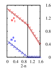
Figure 3: (Color online) Left panel: The different contributions to the variational energy as a function of doping for $U/D=1$ and per lattice site $\mathbf{R}$, i.e. summed over both layer. As a reference, the behavior of non-interacting inter- and intra-layer hopping contributions is plotted (dotted lines). In the inset the total energy $E_{var}(n)=E_{var}+\mu n$ is shown: despite the cusp observed in the hopping contributions, the evolution of $E_{var}(n)$ is smooth. Right panel: Occupation of the variational lower and upper bands as function of $n$. Dotted lines represent average occupation of even and odd orbitals.

IV.1 Doping the metal at $U<U_{c}$

As long as $U<U_{c}$, any change of $\mu$ induces a continuous change in the total particle number; a finite compressibility signal of a metallic behavior, as shown in Fig. 2. Alike the uncorrelated case, a cusp appears in the evolution of $n$ at quarter-filling, that we explain seemingly as the depletion of the antibonding band. Indeed, when $U<U_{c}$, the metallic solution evolves just like the non-interacting case. The main effect of interaction is to slightly reduce inter- and intra-layer hopping contributions with respect to their uncorrelated counterparts, as shown in Fig. 3 where we plot the different contributions $E_{hop}$, $E_{\perp}$ and $E_{U}$ to the variational energy. The intra-layer hopping contribution $E_{hop}$ diminishes in absolute value with increasing doping because of the depletion of the bands, as it occurs in the non-interacting system; at quarter-filling it displays a cusp and correspondingly the inter-layer hopping $E_{\perp}$ starts to rapidly decrease, the effects of $U$ being more and more negligible as the low-density regime is approached. In the right panel of Fig. 3 we show the occupancies $n^{0}_{l}$ and $n^{0}_{u}$ of the variational lower and upper bands, respectively, which are obtained by diagonalizing the associated variational Hamiltonian, Eq. (23), and actually coincide with the eigenvalues of the single-particle density matrix. As in the uncorrelated system, the occupancy of the upper band vanishes at quarter filling. We stress the fact that in the present approach these states are variationally determined and may not correspond to the even and odd combinations of the original operators. However, as long as $U<U_{c}$, we find that the average values of bonding and antibonding band occupancies, $n_{e}$ and $n_{o}$, almost coincide with, respectively, $n^{0}_{l}$ and $n^{0}_{u}$.

Concerning superconductivity, we find that the inter-layer order parameter, Eq. (27), is extremely small, practically zero within our numerical precision, see Fig. 4. The intra-layer order parameter strictly follows the inter-layer one, hence is also zero.

IV.2 Doping the VB Mott insulator at $U>U_{c}$

When $U>U_{c}$, i.e. when the half-filled system is insulating, the particle number remains stuck to its half-filled value $n=2$ until $|\mu|\leq|\mu^{*}|\approx(U-U_{c})/2$. This simply follows from the existence of the Mott gap at half-filling. Upon doping, i.e. when $|\mu|>|\mu^{*}|$, a metallic behavior is clearly found. However, within our numerical precision we can not establish whether the evolution from the insulator to the metal occurs smoothly (yet with a diverging compressibility) or through a weak first-order transition. Till the largest value of $U$ we considered, we could not find any appreciable discontinuity in the evolution of $n$ at large doping, unlike for $U<U_{c}$ where a cusp is observed at quarter filling. In addition, contrary to the case $U<U_{c}$, here we find a clear superconducting signal between half and quarter filling, see e.g. the behavior of $\Delta_{\perp}$, Eq. 27, shown in Fig. 4. We note that $\Delta_{\perp}$ has a non-monotonous behavior, first increases quite rapidly with $U$ and for larger values decreases. Like at half-filling, a finite $\Delta_{\perp}$ produces through Eq. (18) also a finite intra-layer $\Delta_{||}$, Eq. 28, not shown here, which happens to have opposite sign.

Let us now consider in detail the energetic balance for $U>U_{c}$ and its differences with respect to $U<U_{c}$. At very large $U$ (not shown), as holes are injected into the system, both intra- and inter-layer hopping contributions first increase in absolute value, then saturate around approximatively quarter-filling, and eventually decrease as the low-density regime is attained, as expected when approaching the bottom of the variational bands. In other words, the behavior at large $U$ between half- and quarter-filling is quite different from the non-interacting case, while becomes quite similar below. This points to a very different influence of a strong interaction close to half-filling and far away from it and, indirectly, emphasizes the role of the superconductivity that we find for $2>n>1$. For $U\gtrsim U_{c}$, i.e. closer to the half-filled metal-insulator transition, the picture is slightly different, as shown in Fig. 5 for $U/D=3$. To begin with, at small dopings the system gains in intra-layer hopping energy while the inter-layer one seems to be slightly reduced. Remarkably, even if the total energy is, within our numerical accuracy, a smooth function of $n$, both hopping contributions display a discontinuity at $\mu/D\simeq 1.28$, which corresponds to a local density of $n\approx 1.27$. Here the occupation of the upper variational band goes to zero (cfr. right panel of Fig. 5), even though nothing similar occurs in the occupation of the physical antibonding band. At this filling fraction, the inter-layer hopping energy gain has an upward jump, contrary to the intra-layer one, even though further doping leads to a reduction of both. A drop in the amplitude of the superconducting order parameter $\Delta_{\perp}$ is also found at this point. Further doping diminishes $\Delta_{\perp}$, which vanishes approximatively at quarter filling. A similar feature is observed in another quantity. Indeed, just like $n^{0}_{l}$ and $n^{0}_{u}$ may not correspond to the occupation of the bonding and antibonding bands, $n^{0}=n^{0}_{l}+n^{0}_{u}$, which is the average density of the BCS-like variational wavefunction, may differ from the physical one. In the inset of Fig. 4 we show their difference for $U/D=3$. We observe that they actually deviate when superconductivity is found and their difference jumps down abruptly for $n<1.27$.

Figure 4: (Color online) Superconducting inter-layer order parameter $\Delta_{\perp}$ for different $U/D$s. In the inset we plot the difference between the local densities of the BCS variational wavefunction $|\Psi_{0}\rangle$ and of the actual one $|\Psi_{G}\rangle$, at $U/D=3$.

Figure 5: (Color online) Left panel: Contributions to the variational energy as function of doping for $U/D=3$. In the inset the total energy $E_{var}(n)=E_{var}+\mu n$ is shown: despite the discontinuities observed in the hopping contributions, the evolution of $E(n)$ is, to our numerical accuracy, smooth. Right panel: Occupancies of lower, $n^{0}_{l}$ and upper, $n^{0}_{u}$, variational bands as function of $n$. Dotted lines represent average occupation of even, $n_{e}$, and odd, $n_{o}$, orbitals. Note that the insulating phase at half-filling is identified by the lower band fully occupied and the upper one empty. The latter empties again for doping $2-n>0.73$.

V Conclusions

In this work we have studied by means of an extension of the Gutzwiller approximation the effect of doping a bilayer Hubbard model. We have considered a value of the inter-layer hopping $t_{\perp}$ such that, at half-filling, the model should undergo a direct transition at $U=U_{c}$ from a metal to a non-magnetic Mott insulator, a valence bond crystal consisting of inter-layer dimers. This choice offers the opportunity to study how a valence bond crystal liquefies either by reducing the Coulomb repulsion keeping the density fixed at one electron per site, or by adding mobile holes. The melting upon decreasing $U$ was already shown Fabrizio (2007) to lead to a superconducting phase intruding between the valence bond insulator at large $U>U_{c}$ and the normal metal at weak $U\ll U_{c}$. Here we show that superconductivity arises also upon melting the valence bond crystal by doping. In other words, the superconducting dome that exists at half-filling close to $U_{c}$ extends into a whole region at finite doping. The maximum superconducting signal is found at 20% doping, and beyond that it smoothly diminishes, disappearing roughly at quarter filling within our choice of parameters. These results are appealing as they show that the well established behavior of a two-leg Hubbard ladder Fabrizio (2007); Balents and Fisher (1996); Schulz (1999); Sierra et al. (1998) seems to survive in higher dimensions, actually in the infinite-dimension limit where our Gutzwiller approximation becomes exact. It is obvious that, in spite of all improvements of the Gutzwiller variational approach, to which we contribute a bit with this work, this method remains variational hence not exact. Therefore it is still under question if superconductivity indeed arises by metallizing the valence bond Mott insulating phase of a Hubbard bilayer, which we believe is an important issue of broader interest than the simple bilayer model we have investigated Capone et al. (2004). There are actually quantum Monte Carlo simulations Scalettar et al. (1994); Bulut et al. (1992); dos Santos (1995); Bouadim et al. (2008) that partially support our results as they show a pronounced enhancement of superconducting fluctuations close to the half-filled Mott insulator. However a true superconducting phase is still unaccessible to the lowest temperatures that can be reached by quantum Monte Carlo. On the other hand, dynamical mean field calculations, that can access zero temperature phases, did not so far looked for superconductivity Fuhrmann et al. (2006); Kancharla and Okamoto (2007). Therefore we think it would be worth pursuing further this issue.

References

- Gutzwiller (1963) M. C. Gutzwiller, Phys. Rev. Lett. 10, 159 (1963).
- Gutzwiller (1964) M. C. Gutzwiller, Phys. Rev. 134, A923 (1964).
- Gutzwiller (1965) M. C. Gutzwiller, Phys. Rev. 137, A1726 (1965).
- Sorella (2005) S. Sorella, Phys. Rev. B 71, 241103 (2005).
- Müller-Hartmann (1989) E. Müller-Hartmann, Z. Phys. B: Condens. Matter 76, 211 (1989).
- Metzner and Vollhardt (1987) W. Metzner and D. Vollhardt, Phys. Rev. Lett. 59, 121 (1987).
- Metzner and Vollhardt (1988) W. Metzner and D. Vollhardt, Phys. Rev. B 37, 7382 (1988).
- Bünemann et al. (1998) J. Bünemann, W. Weber, and F. Gebhard, Phys. Rev. B 57, 6896 (1998).
- Kotliar and Ruckenstein (1986) G. Kotliar and A. E. Ruckenstein, Phys. Rev. Lett. 57, 1362 (1986).
- Bunemann and Gebhard (2007) J. Bunemann and F. Gebhard, Phys. Rev.B 76, 193104 (2007).
- Lechermann et al. (2007) F. Lechermann, A. Georges, G. Kotliar, and O. Parcollet, Phys. Rev. B 76, 155102 (2007).
- Brinkman and Rice (1970) W. F. Brinkman and T. M. Rice, Phys. Rev. B 2, 4302 (1970).
- Georges et al. (1996) A. Georges, G. Kotliar, W. Krauth, and M. J. Rozenberg, Rev. Mod. Phys. 68, 13 (1996).
- Anisimov et al. (1997) V. I. Anisimov, F. Aryasetiawan, and A. Lichtenstein, J. Phys.: Condens. Matter 9, 767 (1997).
- Capello et al. (2005) M. Capello, F. Becca, M. Fabrizio, S. Sorella, and E. Tosatti, Phys. Rev. Lett. 94, 026406 (2005).
- Bünemann et al. (2005) J. Bünemann, F. Gebhard, T. Ohm, S. Weiser, and W. Weber, in Frontiers in Magnetic Materials, edited by A. Narlikar (Springer, Berlin, 2005), pp. 117–151.
- Attaccalite and Fabrizio (2003) C. Attaccalite and M. Fabrizio, Phys. Rev. B 68, 155117 (2003).
- Fabrizio (2007) M. Fabrizio, Phys. Rev. B 76, 165110 (2007).
- Barone et al. (2007) P. Barone, R. Raimondi, M. Capone, C. Castellani, and M. Fabrizio, Europhys. Lett. 79, 47003 (2007).
- Borghi et al. (2009) G. Borghi, M. Fabrizio, and E. Tosatti, Phys. Rev. Lett. 102, 066806 (2009).
- Deng et al. (2009) X. Deng, L. Wang, X. Dai, and Z. Fang, Phys. Rev. B 79, 075114 (2009).
- Bickers et al. (1989) N. E. Bickers, D. J. Scalapino, and S. R. White, Phys. Rev. Lett. 62, 961 (1989).
- Kotliar and Liu (1988) G. Kotliar and J. Liu, Phys. Rev. B 38, 5142 (1988).
- Gros (1988) C. Gros, Phys. Rev. B 38, 931 (1988).
- Paramekanti et al. (2004) A. Paramekanti, M. Randeria, and N. Trivedi, Phys. Rev. B 70, 054504 (2004).
- Sorella et al. (2002) S. Sorella, G. B. Martins, F. Becca, C. Gazza, L. Capriotti, A. Parola, and E. Dagotto, Phys. Rev. Lett. 88, 117002 (2002).
- Anderson et al. (2004) P. W. Anderson, P. A. Lee, M. Randeria, T. M. Rice, N. Trivedi, and F. C. Zhang, J. Phys.: Condens. Matter 16, R755 (2004).
- Lichtenstein and Katsnelson (2000) A. I. Lichtenstein and M. I. Katsnelson, Phys. Rev. B 62, R9283 (2000).
- Potthoff et al. (2003) M. Potthoff, M. Aichhorn, and C. Dahnken, Phys. Rev. Lett. 91, 206402 (2003).
- Senechal et al. (2000) D. Senechal, D. Perez, and M. Pioro-Ladriere, Phys. Rev. Lett. 84, 522 (2000).
- Kotliar et al. (2001) G. Kotliar, S. Y. Savrasov, G. Pálsson, and G. Biroli, Phys. Rev. Lett. 87, 186401 (2001).
- Maier et al. (2005) T. Maier, M. Jarrell, T. Pruschke, and M. H. Hettler, Rev. Mod. Phys. 77, 1027 (2005).
- Dahnken et al. (2004) C. Dahnken, M. Aichhorn, W. Hanke, E. Arrigoni, and M. Potthoff, Phys. Rev. B 70, 245110 (2004).
- Strong and Millis (1994) S. P. Strong and A. J. Millis, Phys. Rev. B 50, 9911 (1994).
- Shelton et al. (1996) D. G. Shelton, A. A. Nersesyan, and A. M. Tsvelik, Phys. Rev. B 53, 8521 (1996).
- Balents and Fisher (1996) L. Balents and M. P. A. Fisher, Phys. Rev. B 53, 12133 (1996).
- Sierra et al. (1998) G. Sierra, M. A. Martín-Delgado, J. Dukelsky, S. R. White, and D. J. Scalapino, Phys. Rev. B 57, 11666 (1998).
- Fabrizio (1993) M. Fabrizio, Phys. Rev. B 48, 15838 (1993).
- Schulz (1999) H. J. Schulz, Phys. Rev. B 59, R2471 (1999).
- Anderson (1987) P. W. Anderson, Science 235, 1196 (1987).
- Sandvik and Scalapino (1994) A. W. Sandvik and D. J. Scalapino, Phys. Rev. Lett. 72, 2777 (1994).
- Scalettar et al. (1994) R. T. Scalettar, J. W. Cannon, D. J. Scalapino, and R. L. Sugar, Phys. Rev. B 50, 13419 (1994).
- dos Santos (1995) R. R. dos Santos, Phys. Rev. B 51, 15540 (1995).
- Wang et al. (2006) L. Wang, K. S. D. Beach, and A. W. Sandvik, Phys. Rev. B 73, 014431 (2006).
- Bouadim et al. (2008) K. Bouadim, G. G. Batrouni, F. Hébert, and R. T. Scalettar, Phys. Rev. B 77, 144527 (2008).
- Fuhrmann et al. (2006) A. Fuhrmann, D. Heilmann, and H. Monien, Phys. Rev. B 73, 245118 (2006).
- Kancharla and Okamoto (2007) S. S. Kancharla and S. Okamoto, Phys. Rev. B 75, 193103 (2007).
- Bulut et al. (1992) N. Bulut, D. J. Scalapino, and R. T. Scalettar, Phys. Rev. B 45, 5577 (1992).
- Lanatà et al. (2008) N. Lanatà, P. Barone, and M. Fabrizio, Phys. Rev. B 78, 155127 (2008).
- Capone et al. (2004) M. Capone, M. Fabrizio, C. Castellani, and E. Tosatti, Phys. Rev. Lett. 93, 047001 (2004).