Spectroscopy of drums and quantum billiards: perturbative and non-perturbative results

Abstract

We develop powerful numerical and analytical techniques for the solution of the Helmholtz equation on general domains. We prove two theorems: the first theorem provides an exact formula for the ground state of an arbirtrary membrane, while the second theorem generalizes this result to any excited state of the membrane. We also develop a systematic perturbative scheme which can be used to study the small deformations of a membrane of circular or square shapes. We discuss several applications, obtaining numerical and analytical results.

I Introduction

The calculation of the frequencies of a drum of arbitrary shape is a problem of formidable difficulty. In fact, the exact solutions to the Helmholtz equation are known only in special cases, namely for the equilateral triangle, for rectangles and for circles and ellipses, where they are expressed in terms of trigonometric, Bessel and Mathieu functions. For general shapes, including those obtained performing small perturbations of the domains just mentioned, exact results are not available. In these cases one is forced to use approximate methods, which can be either analytical or numerical.

The same problem holds for a quantum billiard, which is defined as a region of space where a point particle (for example an electron) is moving freely, not being allowed to escape. This is the quantum analog of a classical billiard where a particle only interacts when colliding elastically with the walls of the billiard, changing its trajectory. The Schrödinger equation in this case reduces to the Helmholtz equation used to describe the drum.

The study of quantum billiards requires the calculation of a large number of energy levels, which are needed to extract the statistical distribution of the the level spacing $s_{n}=E_{n+1}-E_{n}$. On theoretical grounds it is expected to obtain different statistical distributions if the corresponding classical billiard is either integrable or chaotic.

Given the interest in calculating both the low and high parts of the spectrum, different approaches have been developed over the years to obtain approximate solutions to the general problem. We may divide them into two categories: numerical and analytical methods. It is outside of the scope of this paper to give a full account of all different approaches which have been used before for this problem; we rather prefer to mention a selected number of works which we find representative and which can the source for additional reading. The reader interested in finding more details and references may find useful to check the bibliography of the papers that we mention; in particular, a very useful source of information on this problem is the beautiful paper by Kuttler and Sigillito  Kuttler84 , which contains $142$ references and which reports both numerical and analytical results.

Among the numerical methods used to solve the Helmholtz equation we mention:

• the method of particular solutions (also known as Point Matching Method) of Fox, Henrici and Moler  Fox67 (a recent improvement of this method is discussed in ref. Betcke05 );

• the method of fundamental solutions of Bogomolny  Bogomolny85 ;

• domain decomposition method of ref. Descloux83 (a recent application to isospectral drum is contained in Driscoll97 );

• the conformal mapping method (CMM) of Robnik Robnik84 ;

• the plane wave decomposition method (PWDM) of Heller  Heller91 ;

• boundary integral methods (BIM) (see for example  Kostin97 ; Heller04 );

• the method of Vergini and Saraceno  Vergini95 ;

• the expansion method of Kaufman, Kostin and Schulten Kaufman99 ;

• finite element methods (FEM), see for example DeMenezes07 ; Son09 or the multigrid method of Heuveline Heuveline03 ;

• collocation methods (in particular ref. Boyd00 contains a useful introduction to pseudospectral methods): as a special case in this category we mention the conformal collocation method Amore08 ; Amore09 , which will be used in this paper;

• the radial rescaling method of Lijnen08

We now come to the analytical approaches to the solution of the Helmholtz equation, which are essentially based on perturbation theory. It appears in this case that the attempts to perform systematic and precise calculations for the spectrum of arbitrary membranes are fewer and not as successfull as for the numerical methods. In particular Ref. Feshbach53 describes a boundary shape perturbation method, which is expressed in terms of the Green’s function. Ref. Walecka80 describes the arbitrary perturbation of a circular domain which preserves the internal area of a membrane. This first order calculation is originally due to Rayleigh Rayleigh45 . Other perturbative approaches have been introduced in Parker98 ; Read96 ; Bera08 ; Chakraborty09 ; Mendezb05a . Still based on perturbation theory is the $\lambda$-expansion used by Molinari in Molinari97 to deal with regular polygonal membranes. None of the methods mentioned above has been applied to a systematic calculation of the spectrum, but rather of few selected levels. As a matter of fact, we are not aware of calculations in the literature for the whole spectrum of a drum, even slightly perturbed with respect to a solvable problem. In a different context, the study of chaos in atomic nuclei, perturbation theory has also been used to study the statistical fluctuations of ground-state and binding energies Molinari04 .

Interestingly, it seems that the analytical methods have received considerably less attention than the numerical methods. The development of a systematic approach to perturbation theory for membranes (quantum billiards) of arbitrary shape is thus one the goals of the present paper.

The paper is organized as follows: in section II we describe two numerical approaches to the solution of the Helmholz equation on arbitrary domains which are based on the use of conformal mapping (these are a new version of the CMM of ref. Robnik84 and the CCM of ref. Amore08 ); in section III we develop two different analytical approaches to the solution of the problem: in the first approach, which is nonperturbative, we prove two theorems which provide, general expressions for the energies of the ground state or of an arbitrarily excited state; in the second approach, which is perturbative, we obtain a systematic expansion for the energies of an arbitrary membrane. In section IV we apply the methods of sections II and III to several non trivial examples, which are helpful to illustrate the power of the techniques developed in this paper. Finally in section V we draw our conclusions.

All the numerical calculations have been carried out using Mathematica 7 Wolfram .

II Numerical methods

In this section we describe two different numerical methods: in the first part we introduce and modify the conformal mapping method (CMM), which was originally developed by Robnik Robnik84 ; in the second part we discuss the conformal collocation method (CCM), which has been developed by the author in a recent paper Amore08 .

II.1 Conformal mapping method

We briefly describe the conformal mapping method of Ref. Robnik84 . The same notation of that paper is used here. $\mathcal{D}$ is the domain of the billiard whose boundary is given by an analytic curve in the $(u,v)$ plane. The quantum states of a particle confined in $\mathcal{D}$ are described by the hamiltonian

$$\hat{H}=-\frac{\hbar^{2}}{2m}\left[\frac{\partial^{2}}{\partial u^{2}}+\frac{\partial^{2}}{\partial v^{2}}\right]$$ (1)

with Dirichlet boundary conditions on $\mathcal{D}$. In the following we will use $\hbar^{2}/2m=1$.

As explained in ref. Robnik84 a conformal tranformation can be used to map the original region $\mathcal{D}$ onto the unit disk:

$$w=f(z)$$ (2)

where $w=u+iv$ and $z=x+iy$. Actually, using Riemann mapping theorem, one may choose the mapping function $f(z)$ so that $\mathcal{D}$ is mapped to an arbitrary simply connected region of the plane, which we call $\Omega$. Here we choose $\Omega$ to be a square of side $2$. Upon performing the conformal mapping the operator in eq. (1) transforms as

$$\hat{H}\rightarrow-\Sigma^{-1}\ \left[\frac{\partial^{2}}{\partial x^{2}}+\frac{\partial^{2}}{\partial y^{2}}\right]\ ,$$ (3)

where we have defined

$$\Sigma\equiv\left|\frac{df}{dz}\right|^{2}\ .$$ (4)

We therefore obtain the eigenvalue equation

$$\Delta\psi(x,y)+E\Sigma(x,y)\psi(x,y)=0\ .$$ (5)

If we assume Dirichlet boundary conditions the eigenfunctions $\psi(x,y)$ may be conveniently expressed in the orthonormal basis of the eigenfunctions of the laplacian on the square $\Omega$ as:

$$\Phi_{n_{x},n_{y}}(x,y)=\sin\left(\frac{n_{x}\pi}{2}(x+1)\right)\ \sin\left(\frac{n_{y}\pi}{2}(y+1)\right)\ ,$$ (6)

with $n_{x},n_{y}=1,2,\dots,\infty$. Von Neumann boundary conditions could be also studied by using the appropriate basis. We do not consider this case here.

The eigenvalues corresponding to the wavefunctions of eq. (6) are

$$\varepsilon_{n_{x},n_{y}}=\frac{\pi^{2}}{4}\left(n_{x}^{2}+n_{y}^{2}\right)\$$ (7)

and we may write

$$\psi(x,y)=\sum_{n_{x}=1}^{\infty}\sum_{n_{y}=1}^{\infty}c_{n_{x},n_{y}}\Phi_{n_{x},n_{y}}(x,y)\ .$$ (8)

By using the orthogonality of the $\Phi$ we obtain the equations

$$c_{n^{\prime}_{x},n^{\prime}_{y}}\varepsilon_{n^{\prime}_{x},n^{\prime}_{y}}+E\sum_{n_{x},n_{y}}c_{n_{x},n_{y}}\Sigma_{n_{x},n_{y};n^{\prime}_{x},n^{\prime}_{y}}=0$$ (9)

where

$$\Sigma_{n_{x},n_{y};n^{\prime}_{x},n^{\prime}_{y}}\equiv\int_{\Omega}dxdy\ \Phi^{*}_{n^{\prime}_{x},n^{\prime}_{y}}(x,y)\Sigma(x,y)\Phi_{n_{x},n_{y}}(x,y)\ .$$ (10)

In order to convert eq. (9) into a matrix equation we may identify a state in the box using a single integer index

$$k=n_{y}+Nn_{y}\ ,$$ (11)

where $1\leq k\leq N^{2}$ and $N^{2}$ is the number of states to which we have limited the sums in eq. (9) . We may also invert this relation to obtain

$$n_{x}=1+\left[\frac{k}{N+\eta}\right]\ \ ,\ \ n_{y}=k-N\left[\frac{k}{N+\eta}\right]\ ,$$ (12)

where $\left[a\right]$ is the integer part of a real number $a$ and $\eta\rightarrow 0^{+}$.

Using these conventions eq. (9) may now be cast in the form

$$\left[\frac{1}{E}\ \delta_{kk^{\prime}}+\frac{1}{\varepsilon_{k^{\prime}}}\Sigma_{kk^{\prime}}\right]c_{k}=0\ ,$$ (13)

with $1\leq k\leq N^{2}$.

The solution of this equation requires the calculation of a large number of integrals $\Sigma_{kk^{\prime}}$, which is the most time consuming part of the method, as explained in Ref. Robnik84 . Moreover, for large values of the indices in eq. (10) the integrands are rapidly oscillating functions, which are more difficult to calculate numerically.

The calculation however may be done quite efficiently if the conformal map $f(z)$ is a polynomial or if it can be approximated with good precision by a polynomial, i.e. by the first few terms of its Taylor series around $z=z_{0}$, with $z_{0}\in\mathcal{D}$. In such a case we may express $\Sigma(x,y)$ as

$$\Sigma(x,y)=\sum_{n=0}^{\infty}\sum_{m=0}^{\infty}\kappa_{nm}x^{n}y^{m}$$ (14)

and thus obtain

$$\Sigma_{n_{x},n_{y};n^{\prime}_{x},n^{\prime}_{y}}=\sum_{n=0}^{\infty}\sum_{m=0}^{\infty}\kappa_{nm}\mathcal{Q}_{n_{x}n^{\prime}_{x}n}\ \mathcal{Q}_{n_{y}n^{\prime}_{y}m}\$$ (15)

where we have defined

$$\mathcal{Q}_{nmk}\equiv\int_{-1}^{+1}dx\ x^{k}\ \sin\left(\frac{n\pi}{2}(x+1)\right)\ \sin\left(\frac{m\pi}{2}(x+1)\right).$$

The analytical calculation of these integrals may be done quite efficiently using the recurrence relations for the $\mathcal{Q}_{nmk}$ given in appendix A. Recurrence relations for the integrals which are relevant for the von Neumann boundary conditions, $\mathcal{R}_{nmk}$, are also obtained.

II.2 Conformal collocation method

An alternative strategy for the solution of the Helmholtz equation is to use a collocation approach, as explained in Ref. Amore08 . We briefly review this approach.

As we have seen in the previous section the homogeneous Helmholtz equation on a domain $\mathcal{D}$ may be mapped to an inhogeneous Helmholtz equation on a ”simpler” domain $\Omega$ (which in this paper we assume to be a square of side $2$). The resulting equation, eq. (5), may then be written in the equivalent form

$$-\frac{1}{\Sigma(x,y)}\Delta\psi(x,y)=E\psi(x,y)\ .$$ (16)

The discretization of this equation proceeds as follows (more detail can be found in Ref. Amore08 ): first, we introduce a set of functions, the little sinc functions (LSF) of ref. Amore07 , $s_{k}(h,N,x)$, which are defined on $x\in(-1,1)$ and obey Dirichlet bc at the borders (LSF corresponding to more general boundary conditions are obtained in ref. Amore09c ) :

$$s_{k}(h,N,x) \equiv \frac{1}{2N}\left\{\frac{\sin\left(\left(1+\frac{1}{2N}\right)\ \frac{\pi}{h}(x-kh)\right)}{\sin\left(\frac{\pi}{2Nh}(x-kh)\right)}\right.$$ (17)

$$- \left.\frac{\cos\left(\left(1+\frac{1}{2N}\right)\ \frac{\pi}{h}(x+kh)\right)}{\cos\left(\frac{\pi}{2Nh}(x+kh)\right)}\right\}\ .$$

For a given $N$ (integer) there are $N-1$ of these functions, each peaked (with value 1) at a point $x_{k}=kh$ ($h=2/N$ is the spacing of the uniform grid which these functions introduce) and vanishing at the remaining grid points $x_{j}=jh$, $j\neq k$. A function $f(x)$ obeying Dirichlet bc may be interpolated using the $s_{k}(h,N,x)$ as

$$f(x)\approx\sum_{k=-N/2+1}^{N/2-1}f(x_{k})s_{k}(h,N,x)\ .$$ (18)

In a similar way we may derive twice this expression to obtain

$$\frac{d^{2}f(x)}{dx^{2}} \approx \sum_{k=-N/2+1}^{N/2-1}f(x_{k})\ \frac{d^{2}s_{k}(x)}{dx^{2}}$$ (19)

$$\approx \sum_{k=-N/2+1}^{N/2-1}\sum_{j=-N/2+1}^{N/2-1}f(x_{k})\ \left.\frac{d^{2}s_{k}(x)}{dx^{2}}\right|_{x_{j}}s_{j}(h,N,x)$$

$$\equiv \sum_{k=-N/2+1}^{N/2-1}\sum_{j=-N/2+1}^{N/2-1}f(x_{k})\ c_{kj}^{(2)}\ s_{j}(h,N,x),$$

where in the last line we have introduced the matrix $c_{kj}^{(2)}\equiv\left.\frac{d^{2}s_{k}(x)}{dx^{2}}\right|_{x_{j}}$, which provides a representation for the second derivative operator on the grid. Notice that these matrix elements are known analytically. The discretization of eq. (16) is now straightforward: for simplicity we consider the one-dimensional version of this equation and we write

$$-\frac{1}{\Sigma(x)}\frac{d^{2}}{dx^{2}}s_{k}(h,N,x)\approx-\sum_{j}\frac{1}{\Sigma(x_{j})}\ c_{kj}^{(2)}\ s_{j}(h,N,x)$$ (20)

which provides an explicit representation of the operator $\hat{O}\equiv-\frac{1}{\Sigma(x)}\frac{d^{2}}{dx^{2}}$ on the uniform grid.

If we want to generalize these results to two dimensions, we may consider the set of functions which are obtained from the direct product of the set of functions in the $x$ and $y$ directions, i.e. $s_{k}(h,N,x)s_{k^{\prime}}(h,N,x)$. Notice that we are assuming that the number of elements in the two directions is the same although different values could be considered if needed. Clearly the representation of an operator on the grid in terms of these functions will depend on four indices (the two integer indices corresponding to the initial point on the grid and the two integers indices corresponding to the final point on the grid). However we may identify a specific point on the grid with a single integer

$$K=k^{\prime}+\frac{N}{2}+(N-1)\left(k+\frac{N}{2}-1\right)\ .$$ (21)

where $1\leq K\leq(N-1)^{2}$. This relation is easily inverted to give:

$$k = 1-\frac{N}{2}+\left[\frac{K}{N-1+\eta}\right]$$ (22)

$$k^{\prime} = K-\frac{N}{2}-(N-1)\left[\frac{K}{N-1+\eta}\right]\ ,$$ (23)

where $\left[a\right]$ is the integer part of $a$ and $\eta\rightarrow 0^{+}$.

Using these results one may easily generalize eqn. (20) to two dimensions as

$$- \frac{1}{\Sigma(x,y)}\Delta s_{k}(h,N,x)s_{k^{\prime}}(h,N,y)=-\sum_{jj^{\prime}}\frac{1}{\Sigma(x_{j},y_{j^{\prime}})}$$ (24)

$$\times \left[c_{kj}^{(2)}\delta_{k^{\prime}j^{\prime}}+\delta_{kj}c_{k^{\prime}j^{\prime}}^{(2)}\right]s_{j}(h,N,x)s_{j^{\prime}}(h,N,y)$$

from which we easily obtain the representation of $\hat{O}\equiv-\frac{1}{\Sigma(x,y)}\Delta$ on the grid :

$$O_{KK^{\prime}}=-\frac{1}{\Sigma(x_{j},y_{j^{\prime}})}\left[c_{kj}^{(2)}\delta_{k^{\prime}j^{\prime}}+\delta_{kj}c_{k^{\prime}j^{\prime}}^{(2)}\right]\ .$$ (25)

We underline some useful features of this expression:

• the matrix corresponding to $\left[c_{kj}^{(2)}\delta_{k^{\prime}j^{\prime}}+\delta_{kj}c_{k^{\prime}j^{\prime}}^{(2)}\right]$ is the representation of the 2D laplacian operator on the uniform grid in a square of side $L=2$; this matrix is ”universal”, i.e. not specific to the particular problem one is solving, and sparse.

• the matrix corresponding to $\frac{1}{\Sigma(x_{j},y_{j^{\prime}})}$ is specific to the domain $\mathcal{D}$ since $\Sigma$ is related to the conformal map; however this matrix is diagonal and therefore only $N-1$ elements need to be calculated;

• the matrix $O$ is a nonsymmetrical real square matrix whose eigenvalues are real.

• no integrals need to be calculated, since $\Sigma$ is simply evaluated on the grid points. In this case one does not need to approximate the map with a polynomial in $z$.

Because of the features above, the optimal computational strategy consists of calculating the matrices for the discretized laplacian on $\Omega$ for grids of different sizes. Typically, this is the most time consuming task but it only needs to be done once, since these matrices are common to all problems and therefore they can be stored and used when needed without having to recalculate them. When a particular conformal map is chosen, one only needs to calculate the $N-1$ diagonal elements of $\Sigma$, which has a much more limited computational cost. The matrix representation for $\hat{O}$ is thus obtained quite effectively and selected eigenvalues (eigenvectors) may be calculated rapidly. We will discuss some applications of this approach in Section IV.

III Analytical methods

In this section we derive useful analytical approximations for the energies of a particle confined in a two dimensional region. In the first part we obtain a systematic approximation to the ground state energy and wave function (or more in general to the lowest state in each symmetry class of the problem): this expansion is really non-perturbative and it is proved to converge to the exact values; in the second part we obtain the analytical expression for the spectrum of an arbitrary two dimensional region, worked out in perturbation theory up to third order.

III.1 Nonperturbative formulas

We will now derive a general formula for the ground state of a drum obeying Helmholtz equation (5) or the equivalent equation (16).

As noticed before the conformal map has allowed to convert the original homogeneous Helmholtz equation, defined on a domain $\mathcal{D}$, into an inhomogenous Helmholtz equation, defined on a ”simpler” domain $\Omega$, which in the present case we will assume to be a square of side $2$.

We make few observations regarding the composite operator $\hat{O}=-\frac{1}{\Sigma(x,y)}\Delta$, which will help us to devise a suitable approach to finding approximations to the states of eq.(16):

• the operator $\hat{O}$ is non-hermitian, $\hat{O}^{\dagger}\neq\hat{O}$. This confirms the observation made in the previous section that the matrix representing the operator on the uniform grid is real and non-symmetrical.

• the operator $\hat{O}$ may be cast in a manifestly hermitian form by considering its symmetrized form

  $$\hat{O}^{(sym)}=\frac{1}{\sqrt{\Sigma}}(-\Delta)\frac{1}{\sqrt{\Sigma}}\ .$$ (26)

  In the framework of the Conformal Collocation Method (CCM) of the previous section, the matrix representing this operator on a uniform grid is symmetrical and hermitian. Moreover its eigenvalues coincide with those of the unsymmetrized matrix. From now on we will always work with $\hat{O}^{(sym)}$ and therefore we will omit the superscript. It is interesting to notice that the form that we have found for $\hat{O}^{(sym)}$ has been proposed by Zhu and Kroemer in Zhu83 , discussing the problem of the connection rules for effective mass wave functions across abrupt heterojunctions. A discussion of kinetic operators containing more general position dependent effective mass terms is discussed in vonRoos83 .

• $\Omega$ is a two-dimensional domain on which the spectrum (energies and wave functions) of the negative laplacian operator is known exactly, i.e. a square (rectangle) or a circle.

• the eigenvalues of $\hat{O}$ are definite positive if we assume Dirichlet boundary conditions: the inverse operator $\hat{O}$ exists. For von Neumann boundary conditions a state with zero energy is present and one needs to define the invertible operator

  $$\hat{O}_{\eta}=\frac{1}{\sqrt{\Sigma}}(-\Delta+\eta)\frac{1}{\sqrt{\Sigma}}\ .$$ (27)

  where $\eta\rightarrow 0^{+}$ is a positive infinitesimal parameter.

• the spectrum of $\hat{O}$ is not bounded from above, i.e. there is an infinite number of states, of arbitrarily high energy;

• the spectrum of the inverse operator $\hat{O}^{-1}$ is bounded from above, the largest eigenvalue being the reciprocal of the lowest eigenvalue of $\hat{O}$ (of course there is still an infinite number of states which become denser and denser as the eigenvalues approach zero). The spectrum of $\hat{O}_{\eta}^{-1}$ corresponding to von Neumann boundary conditions is also bounded from above, although its largest eigenvalue tends to infinity as $\eta$ tends to zero.

To simplify the notation in the following we will write $\hat{O}_{\eta}$ as simply $\hat{O}$, implicitly assuming that an infinitesimal positive shift $\eta$ is used if von Neumann bc are used.

We are now in position of stating the following Theorem:

Theorem 1

Let $|\Psi_{0}\rangle$ be the exact ground state of the operator $\hat{O}$ and $|\Psi\rangle$ be an arbitrary state with nonzero overlap with $|\Psi_{0}\rangle$. Then the lowest mode of the Helmholtz equation (16) is given by

$$|\Psi_{0}\rangle=\lim_{n\rightarrow\infty}\left[\hat{O}^{-1}\right]^{n}|\Psi\rangle\ .$$ (28)

where $\hat{O}^{-1}=\sqrt{\Sigma}(-\Delta+\eta)^{-1}\sqrt{\Sigma}$ and $\Sigma\equiv\left|\frac{df}{dz}\right|^{2}$ ($f(z)$ is the conformal map which maps $\mathcal{D}$ into $\Omega$). More in general, if $|\Psi\rangle$ is orthogonal to the first $n$ states of eq.(16) then the resulting state converges to the $n+1$ excited state.

The proof of this theorem is easy: for simplicity we limit to Dirichlet bc and therefore set $\eta=0$ (the case of von Neumann bc is obtained straightforwardly, working with a nonzero $\eta$).

Given an arbitrary state $|\Psi\rangle$, we may decompose it in terms of the eigenstates of $\hat{O}$, $|\Psi_{n}\rangle$, and write $|\Psi\rangle=\sum_{n=0}^{\infty}a_{n}|\Psi_{n}\rangle$.

By applying the inverse operator to this state we obtain

$$\hat{O}^{-1}|\Psi\rangle=\sum_{n=0}^{\infty}\frac{a_{n}}{E_{n}}|\Psi_{n}\rangle$$ (29)

where $E_{n}$ are the eigenvalues of $\hat{O}$. These eigenvalues are positive definite, $E_{n}>0$, for all values of $n$. For this reason the component of $|\Psi_{0}\rangle$ in this new state has been amplified with respect to all the other components $|\Psi_{n\geq 1}\rangle$. Therefore repeated applications of the inverse operator will further suppress these components and the resulting state will converge to the true ground state of $\hat{O}$. This concludes our demonstration.

What we have described so far is actually an implementation of the well known Power Method OLeary79 for an infinite dimensional matrix, with positive definite eigenvalues which are bounded from above.

There are several aspects which make the present implementation of the Power Method particularly appealing:

• the convergence rate of the algorithm depends on the ratio of $E_{1}/E_{0}$, becoming slower when $E_{0}$ and $E_{1}$ are not well separated. An upper bound to this ratio is provided by the Payne-Polya-Weinberger conjecture PPW1 ; PPW2

  $$\frac{E_{1}}{E_{0}}\leq\left.\frac{E_{1}}{E_{0}}\right|_{disk}=\left(\frac{j_{1,1}}{j_{0,1}}\right)^{2}\approx 2.539$$ (30)

  where $j_{0,1}$ and $j_{1,1}$ are the first positive zeroes of the Bessel functions $J_{0}(x)$ and $J_{1}(x)$. This conjecture has been proved in ref. Benguria91 . On the other hand, it is easy to convince oneself that the ratio will get close to $1$ for elongated domains $\mathcal{D}$, where the longitudinal dimension is much larger then the transverse one. In these cases one may combine the method with a suitable dilatation in order to improve the convergence.

• the ground state of the negative laplacian on $\Omega$ provides an initial guess of good quality (the typical implementation of the Power Method uses a random initial guess);

• in the case of von Neumann bc the initial guess should be chosen orthogonal to the zero energy state, which is trivial.

• we may reasonably expect that the lowest modes of the negative laplacian on $\Omega$, which we call $|n\rangle$, dominate in $|\Psi_{0}\rangle$; therefore we may leave the coefficients of the expansion of the initial guess in terms of the $|n\rangle$ unspecified and use the variational principle to obtain them. In other words we may look for the coefficients which minimize the expectation value of $\hat{O}$ in the state generated with the Power Method.

We now explore explicitly the application of the variational principle to first order. For simplicity we assume $\Omega$ to be a square. Let us choose an arbitrary state $|\chi\rangle$ which can be decomposed in terms of the eigenstates of the Laplacian on a box as

$$|\chi\rangle=\sum_{k}c_{k}^{(0)}|k\rangle.$$ (31)

Notice that the state $|k\rangle=|k_{x},k_{y}\rangle$ is the direct product of the states corresponding to each direction. Similarly we call $\epsilon_{k}$ the eigenvalue of the negative Laplacian on $\Omega$ for this state, $\epsilon_{k}\equiv\frac{\pi^{2}}{4}\left(k_{x}^{2}+k_{y}^{2}\right)$.

Working to first order we obtain an explicit approximate expression for the ground state

$$|\Psi_{0}^{(1)}\rangle = \left[\hat{O}^{-1}\right]|\chi\rangle=\left[\Sigma^{1/2}\left(-\Delta\right)^{-1}\Sigma^{1/2}\right]|\chi\rangle$$ (32)

$$= \sum_{k,l,m=0}^{\infty}\frac{c_{m}^{(0)}}{\epsilon_{l}}|k\rangle\langle k|\Sigma^{1/2}|l\rangle\langle l|\Sigma^{1/2}|m\rangle\ .$$

We may cast this result in the form

$$|\Psi_{0}^{(1)}\rangle = \sum_{k}c_{k}^{(1)}|k\rangle$$ (33)

where

$$c_{k}^{(1)} \equiv \sum_{l,m=0}^{\infty}\frac{c_{m}^{(0)}}{\epsilon_{l}}\langle k|\Sigma^{1/2}|l\rangle\langle l|\Sigma^{1/2}|m\rangle\ .$$ (34)

Using this result we may obtain the first order approximation to the ground state energy :

$$E_{0}^{(1)} = \frac{\langle\Psi_{0}^{(1)}|\hat{O}|\Psi_{0}^{(1)}\rangle}{\langle\Psi_{0}^{(1)}|\Psi_{0}^{(1)}\rangle}\ ,$$ (35)

where

$$\langle\Psi_{0}^{(1)}|\hat{O}|\Psi_{0}^{(1)}\rangle = \sum_{k,l,m=0}^{\infty}\frac{c_{k}^{(0)}c_{m}^{(0)}}{\epsilon_{l}}\langle m|\Sigma^{1/2}|l\rangle\langle l|\Sigma^{1/2}|k\rangle$$ (36)

$$\langle\Psi_{0}^{(1)}|\Psi_{0}^{(1)}\rangle = \sum_{l,l^{\prime},m,m^{\prime}=0}^{\infty}\frac{c_{m}^{(0)}c_{m^{\prime}}^{(0)}}{\epsilon_{l}\epsilon_{l^{\prime}}}\langle m^{\prime}|\Sigma^{1/2}|l^{\prime}\rangle\langle l^{\prime}|\Sigma|l\rangle$$ (37)

$$\times \langle l|\Sigma^{1/2}|m\rangle\ .$$

$E_{0}^{(1)}$ given above provides an upper bound to the true energy $E_{0}$:

$$E_{0}^{(1)}\geq E_{0}.$$ (38)

The coefficients $c_{n}^{(0)}$ may therefore be chosen so that the expectation value of $\hat{O}$ is minimized. Therefore using a suitable number of coefficients in principle one may obtain arbitrarily accurate estimates for $E_{0}$.

If we are willing to trade the accuracy for the simplicity, we may set $c_{0}^{(0)}=1$ and $c^{(0)}_{n\geq 1}=0$: in this case we obtain the approximation

$$E_{0}^{(1)} = \frac{\sum_{l=0}^{\infty}\frac{1}{\epsilon_{l}}\langle 0|\Sigma^{1/2}|l\rangle\langle l|\Sigma^{1/2}|0\rangle}{\sum_{l,l^{\prime}=0}^{\infty}\frac{1}{\epsilon_{l}\epsilon_{l^{\prime}}}\langle 0|\Sigma^{1/2}|l^{\prime}\rangle\langle l^{\prime}|\Sigma|l\rangle\langle l|\Sigma^{1/2}|0\rangle}$$ (39)

which reduces to a quite simple formula when the internal sums are limited to the lowest state

$$E_{0}^{(1)}\approx\frac{\epsilon_{0}}{\langle 0|\Sigma|0\rangle}\ .$$ (40)

In Section IV we will consider few applications of the formulas given above.

The generalization of these results to higher orders is trivial after observing that

$$|\Psi_{0}^{(n)}\rangle = \left[\hat{O}^{-1}\right]|\Psi_{0}^{(n-1)}\rangle=\sum_{k}c_{k}^{(n)}|k\rangle$$ (41)

where

$$c_{k}^{(n)} \equiv \sum_{l,m=0}^{\infty}\frac{c_{m}^{(n-1)}}{\epsilon_{l}}\langle k|\Sigma^{1/2}|l\rangle\langle l|\Sigma^{1/2}|m\rangle\ .$$ (42)

This equation provides a useful recurrence relation for the coefficients $c_{k}$.

For example we have

$$c_{k}^{(2)} \equiv \sum_{l,m=0}^{\infty}\frac{c_{m}^{(1)}}{\epsilon_{l}}\langle k|\Sigma^{1/2}|l\rangle\langle l|\Sigma^{1/2}|m\rangle$$ (43)

$$= \sum_{l,m=0}^{\infty}\frac{c_{m}^{(0)}}{\epsilon_{l}\epsilon_{l^{\prime}}}\langle k|\Sigma^{1/2}|l\rangle\langle l|\Sigma|l^{\prime}\rangle\langle l^{\prime}|\Sigma^{1/2}|m\rangle\ ,$$

where the completeness of states $\sum|k\rangle\langle k|=1$ has been used to obtain the final expression.

The results that we have just obtained for the ground state may also be generalized for the excited states. As a matter of fact we may state the following Theorem:

Theorem 2

Let $|\Psi_{n}^{(d)}\rangle$ be an eigenstate of the operator $\hat{O}$ with degeneracy $d$ and with an eigenvalue $E_{n}$. Let $|\Psi\rangle$ be an arbitrary state with nonzero overlap with at least one of the $|\Psi_{n}^{(d)}\rangle$ and let $\Lambda$ be a real parameter for which $|E_{n}-\Lambda|\ll 1$. Then the state

$$|\Phi\rangle=\lim_{n\rightarrow\infty}\left[\left(\hat{O}-\Lambda\right)^{-2}\right]^{n}|\Psi\rangle\ .$$ (44)

is a linear combination only of the $d$ degenerate states $|\Psi_{n}^{(d)}\rangle$.

The proof of this theorem is analogous to the proof that we have given earlier for the ground state. We just need to notice that the eigenvalues of the operator $\left(\hat{O}-\Lambda\right)^{-2}$ are positive definite and bounded from above. Because of the condition $|E_{n}-\Lambda|\ll 1$ the repeated application of this operator to $|\Psi\rangle$ amplifies the components corresponding to the eigenvalue $E_{n}$ since $1/(E_{n}-\Lambda)^{2}$ is the largest eigenvalue of $\left(\hat{O}-\Lambda\right)^{-2}$. When the limit is taken only the components corresponding to this degenerate eigenvalue survive, which proves the theorem. By choosing other $d-1$ linearly indipendents ansatz and repeating the procedure, we obtain $d$ linearly independent combinations of the degenerate states, which we can use to calculate the matrix elements of $\hat{O}$. The diagonalization of this matrix provides the $d$ eigenstates of interest. Notice that this strategy for calculating arbitrary eigenvalues and eigenvectors of large matrices is discussed in refs. Nash79 ; WZ94 ; GMP95 .

III.2 Perturbation theory

While the previous approach based on the power method provides a systematic approximation to the ground state of a drum of arbitrary shape, an alternative approach consists of applying perturbation theory to obtain the corrections to the energies and wave functions.

Once again our starting point is the symmetrized operator

$$\hat{O}=\frac{1}{\sqrt{\Sigma}}(-\Delta)\frac{1}{\sqrt{\Sigma}}\ ,$$ (45)

which reduces to the negative laplacian for $\Sigma=1$, corresponding to a square of side $L=2$. If we consider small deformations of this square and write

$$\Sigma\rightarrow\Sigma_{\eta}=1+\eta\sigma$$ (46)

where $\sigma\equiv\Sigma-1$ and $\eta$ is a power counting parameter (which at the end of the calculation is set to $1$), which is used to keep track of the different orders in powers of $\sigma$.

Our operator may now be expanded in powers of $\eta$ as

$$\hat{O} \approx \hat{O}_{0}+\eta\hat{O}_{1}+\eta^{2}\hat{O}_{2}+\eta^{3}\hat{O}_{3}+\dots\ ,$$ (47)

where the explicit form of the $\hat{O}_{i}$ may be worked out rather easily:

$$\hat{O}_{0} = -\Delta$$ (48)

$$\hat{O}_{1} = -\frac{1}{2}\left[\sigma(-\Delta)+(-\Delta)\sigma\right]$$ (49)

$$\hat{O}_{2} = \frac{1}{8}\left[2\sigma(-\Delta)\sigma+3\sigma^{2}(-\Delta)+3(-\Delta)\sigma^{2}\right]$$ (50)

$$\hat{O}_{3} = -\frac{3}{16}\left[\sigma^{2}(-\Delta)\sigma+\sigma(-\Delta)\sigma^{2}\right]$$ (51)

$$- \frac{5}{16}\left[\sigma^{3}(-\Delta)+(-\Delta)\sigma^{3}\right]$$

Within perturbation theory we may now calculate the corrections to the eigenvalues and eigenfunctions of our operator $\hat{O}$, keeping in mind that it contains arbitrary powers of $\eta$. The standard scheme of Rayleigh-Schrödinger perturbation theory (RSPT) may be easily adapted to this problem and the contributions up to third order read:

$$E_{n}^{(0)} = \epsilon_{n}$$ (52)

$$E_{n}^{(1)} = \langle n|\hat{O}_{1}|n\rangle$$ (53)

$$E_{n}^{(2)} = \langle n|\hat{O}_{2}|n\rangle+\sum_{k\neq n}\frac{|\langle n|\hat{O}_{1}|k\rangle|^{2}}{\epsilon_{n}-\epsilon_{k}}$$ (54)

$$E_{n}^{(3)} = \langle n|\hat{O}_{3}|n\rangle+2\sum_{k\neq n}\frac{\langle n|\hat{O}_{2}|k\rangle\langle k|\hat{O}_{1}|n\rangle}{\epsilon_{n}-\epsilon_{k}}$$ (55)

$$+ \sum_{k\neq n}\sum_{m\neq n}\frac{\langle n|\hat{O}_{1}|m\rangle\langle m|\hat{O}_{1}|k\rangle\langle k|\hat{O}_{1}|n\rangle}{(\epsilon_{n}-\epsilon_{k})(\epsilon_{n}-\epsilon_{m})}$$

$$- \langle n|\hat{O}_{1}|n\rangle\sum_{k\neq n}\frac{\langle n|\hat{O}_{1}|k\rangle^{2}}{(\epsilon_{n}-\epsilon_{k})^{2}}\ .$$

Notice that the expressions corresponding to orders $\eta^{2}$ and $\eta^{3}$ receive contributions from distinct operators $\hat{O}_{i}$.

We have calculated the perturbative corrections to the energy up to third order for the non-degenerate part of the spectrum:

$$E_{n}^{(1)} = -\epsilon_{n}\langle n|\sigma|n\rangle$$ (56)

$$E_{n}^{(2)} = \epsilon_{n}\langle n|\sigma|n\rangle^{2}+\epsilon_{n}^{2}\sum_{k\neq n}\frac{\langle n|\sigma|k\rangle^{2}}{\epsilon_{n}-\epsilon_{k}}$$ (57)

$$E_{n}^{(3)} = -\epsilon_{n}\langle n|\sigma|n\rangle^{3}+\epsilon_{n}^{3}\langle n|\sigma|n\rangle\sum_{k\neq n}\frac{\langle n|\sigma|k\rangle^{2}}{\omega_{nk}^{2}}$$ (58)

$$- 3\epsilon_{n}^{2}\langle n|\sigma|n\rangle\sum_{k\neq n}\frac{\langle n|\sigma|k\rangle^{2}}{\omega_{nk}}$$

$$- \epsilon_{n}^{3}\sum_{k\neq n}\sum_{m\neq n}\frac{\langle n|\sigma|k\rangle\langle k|\sigma|m\rangle\langle m|\sigma|n\rangle}{\omega_{nk}\omega_{nm}}\ .$$

Details of the derivation of these coefficients are given in the Appendix B.

The expressions above seem to suggest the presence of a term $(-1)^{k}\langle n|\sigma|n\rangle^{k}$ in the perturbative coefficient of order $k$: assuming that this is true, one recovers a geometric series which produces a term $\epsilon_{n}/(1+\langle n|\sigma|n\rangle)$, which, for $n=0$, is precisely the term obtained for the ground state energy working to lowest order, eq. (40).

We may now discuss the extension of these results for degenerate states. Suppose that a state is $d$ times degenerate: in this case the perturbative expansion needs then to be carried out using the eigenstates of the $d\times d$ matrix $\overline{\sigma}_{d}$ of elements $\langle n_{i}|\sigma|n_{j}\rangle$, where $|n_{i}\rangle$ ($i=1,\dots,d$) is one of the degenerate states. With this modification the sums over internal states automatically exclude the degenerate states, given that the interaction does not mix them, and the perturbation expansion is well defined. Notice that if the matrix $\overline{\sigma}_{d}$ is diagonal and proportional to the identity matrix, the degeneracy of the levels will not be lifted by perturbation theory. We will discuss some examples of this in the Section IV considering the spectrum of a circular membrane.

To illustrate how this works in practice we may consider the simplest case, in which the states are twice degenerate. Let us call $|n_{1}\rangle$ and $|n_{2}\rangle$ these states and $\epsilon_{1}$ and $\epsilon_{2}$ their corresponding energies. If we work with perturbations of the square, the states of double degeneracy (which are also the most common states) are states with quantum numbers $(n_{x},n_{y})$ and $(n_{y},n_{x})$.

The eigenvalues of the matrix $\overline{\sigma}_{d=2}$ are:

$$\tilde{\varepsilon}_{1,2} = \frac{1}{2}\left[\langle n_{1}|\sigma|n_{1}\rangle+\langle n_{2}|\sigma|n_{2}\rangle\pm\xi_{12}\right]$$ (59)

where

$$\xi_{12}\equiv\sqrt{\left(\langle n_{1}|\sigma|n_{1}\rangle-\langle n_{2}|\sigma|n_{2}\rangle\right)^{2}+4\langle n_{1}|\sigma|n_{2}\rangle^{2}}\ .$$ (60)

We clearly see that if $\langle n_{1}|\sigma|n_{2}\rangle=0$, then the $\tilde{\varepsilon}_{1,2}$ are degenerate (as anticipated). The eigenvectors of $\overline{\sigma}_{d=2}$ are:

Its eigenvectors are:

$$|\tilde{n}_{1,2}\rangle = \beta_{1}^{(1,2)}|n_{1}\rangle+\beta_{2}^{(1,2)}|n_{2}\rangle\ ,$$ (61)

where

$$\beta_{1}^{(1)} = -\frac{1}{\sqrt{2}}\ \sqrt{1-\frac{\langle n_{1}|\sigma|n_{1}\rangle-\langle n_{2}|\sigma|n_{2}\rangle}{\xi_{12}}}$$ (62)

$$\beta_{2}^{(1)} = \frac{1}{\sqrt{2}}\ \sqrt{1+\frac{\langle n_{1}|\sigma|n_{1}\rangle-\langle n_{2}|\sigma|n_{2}\rangle}{\xi_{12}}}$$ (63)

$$\beta_{1}^{(2)} = \frac{1}{\sqrt{2}}\ \sqrt{1+\frac{\langle n_{1}|\sigma|n_{1}\rangle-\langle n_{2}|\sigma|n_{2}\rangle}{\xi_{12}}}$$ (64)

$$\beta_{2}^{(2)} = -\frac{1}{\sqrt{2}}\ \sqrt{1-\frac{\langle n_{1}|\sigma|n_{1}\rangle-\langle n_{2}|\sigma|n_{2}\rangle}{\xi_{12}}}\ .$$ (65)

We may now explicitly write down the different orders in PT. For example to first order we have

$$E_{n}^{(1)} = -\epsilon_{n}\langle\tilde{n}_{1,2}|\sigma|\tilde{n}_{1,2}\rangle$$ (66)

$$= -\frac{\epsilon_{n}}{2}\left[\langle n_{1}|\sigma|n_{1}\rangle+\langle n_{2}|\sigma|n_{2}\rangle\pm\xi_{12}\right]\ .$$

To second order we have:

$$E_{n}^{(2)} = \epsilon_{n}\langle\tilde{n}_{1,2}|\sigma|\tilde{n}_{1,2}\rangle^{2}+\epsilon_{n}^{2}\sum_{k\neq n}\frac{\langle\tilde{n}_{1,2}|\sigma|k\rangle^{2}}{\epsilon_{n}-\epsilon_{k}}$$ (67)

$$= \frac{\epsilon_{n}}{4}\left[\langle n_{1}|\sigma|n_{1}\rangle+\langle n_{2}|\sigma|n_{2}\rangle\pm\xi_{12}\right]^{2}$$

$$+ \epsilon_{n}^{2}\sum_{k\neq n}\frac{\left(\beta_{1}^{(1,2)}\langle n_{1}|\sigma|k\rangle+\beta_{2}^{(1,2)}\langle n_{2}|\sigma|k\rangle\right)^{2}}{\epsilon_{n}-\epsilon_{k}}$$

We do not write explicitly the formula of the third order which is obtained in a similar fashion.

III.3 Perturbation theory again

Let us now try to obtain perturbative expressions for the energies using a different approach, which uses the theorems of eq. (28) and (44). For simplicity we limit our considerations only to the ground state.

Using eq. (28) we write

$$E_{0}=\lim_{n\rightarrow\infty}\frac{\langle\Psi|\left[O^{-1}\right]^{n-1}|\Psi\rangle}{\langle\Psi|\left[O^{-1}\right]^{n}|\Psi\rangle}\ ,$$ (68)

where

$$\hat{O}^{-1}=\sqrt{1+\eta\sigma}\ \left(-\hat{\Delta}^{-1}\right)\ \sqrt{1+\eta\sigma}\ .$$ (69)

and $|\Psi\rangle$ is an arbitrary state with non-zero overlap with the exact ground state.

The perturbative series for $E_{0}$ is of the form

$$E_{0}^{(PT)}=\sum_{k=0}^{\infty}E_{0}^{(k)}\eta^{k}$$ (70)

and therefore

$$E_{0}^{(k)}=\frac{1}{k!}\left.\frac{\partial^{k}E_{0}^{(PT)}}{\partial\eta^{k}}\right|_{\eta=0}\ .$$ (71)

In taking the derivatives of the expression (68) we need to consider that the state $|\Psi\rangle$ is arbitrary and therefore it may be chosen to be independent of $\eta$. A suitable choice is to pick $|\Psi\rangle$ the ground state of the unperturbed hamiltonian, $-\Delta$.

Let us consider, for example, the first order term:

$$E_{0}^{(1)} = \left.\frac{\partial E_{0}^{(PT)}}{\partial\eta}\right|_{\eta=0}=\left.\lim_{n\rightarrow\infty}\left[\frac{\langle\Psi|\frac{\partial}{\partial\eta}\left[O^{-1}\right]^{n-1}|\Psi\rangle}{\langle\Psi|\left[O^{-1}\right]^{n}|\Psi\rangle}-\frac{\langle\Psi|\left[O^{-1}\right]^{n-1}|\Psi\rangle\langle\Psi|\frac{\partial}{\partial\eta}\left[O^{-1}\right]^{n}|\Psi\rangle}{\langle\Psi|\left[O^{-1}\right]^{n}|\Psi\rangle^{2}}\right]\right|_{\eta=0}\ .$$ (72)

In order to evaluate this expression we only need to consider the terms containing the derivatives, since the remaining terms may already be evaluated at $\eta=0$. For instance

$$\left.\langle\Psi|\left[O^{-1}\right]^{n}|\Psi\rangle\right|_{\eta=0}=\left[E_{0}^{(0)}\right]^{-n}\ .$$ (73)

Let us now consider $\hat{O}^{-n}$ us to order $\eta$:

$$\hat{O}^{-n} \approx (-\Delta)^{-n}+\eta\left[\frac{\sigma}{2}(-\Delta)^{-n}+(-\Delta)^{-1}\sigma(-\Delta)^{-n+1}\right.$$

$$+ \left.\dots+(-\Delta)^{-n+1}\sigma(-\Delta)^{-1}+(-\Delta)^{-n}\frac{\sigma}{2}\right]$$

Therefore

$$\left.\langle\Psi|\frac{\partial}{\partial\eta}\left[O^{-1}\right]^{n}|\Psi\rangle\right|_{\eta=0}=(n+1)\langle\Psi|\sigma|\Psi\rangle\left[E_{0}^{(0)}\right]^{-n}\ .$$ (74)

We thus obtain:

$$E_{0}^{(1)} = \lim_{n\rightarrow\infty}\left[nE_{0}\langle\Psi|\sigma|\Psi\rangle-(n+1)E_{0}\langle\Psi|\sigma|\Psi\rangle\right]$$ (75)

$$= -E_{0}\langle\Psi|\sigma|\Psi\rangle\ ,$$

which agrees with the formula obtained earlier.

IV Applications

In this section we consider several applications of the methods described in the previous sections and compare the results obtained with those in the literature.

IV.1 Unit circle

The exact wave functions and energies of a circular billiard are known analytically and are expressed in terms of the Bessel functions and its zeroes. This example therefore provides an ideal test both for our numerical methods and for our analytical approximations (clearly $\Omega$ in this case is a square). Fig. 1 displays the unit circle which is obtained from a square of side $2$ using a conformal map. The internal lines in the circle correspond to the mapping of a uniform grid on the square. Here the map has been approximated with the Taylor expansion to order $z^{37}$. The effect of this approximation is well under control, since the coefficients decay quickly: for instance, the coefficient of $z^{37}$ is $1.6\times 10^{-11}$. We may roughly expect that the smallest errors that we can obtain in our calculation stopping to this order are of this order of magnitude. Notice that using higher orders in the Taylor expansion makes sense only if one can handle the matrices of the size needed to achieve the extra precision made available by the Taylor expansion.

We have applied both methods described in this paper to this problem, working to different orders. The results obtained for the first three levels are reported in Tables 1 (CMM) and 2 (CCM). In the case of CCM $N^{2}$ is the number of elements of the basis of the square which have been used; in the case of the CCM $N^{2}$ is the number of internal grid points used for the discretization. The reader may notice that the results obtained with the CMM for these states are more precise than those of the CCM for the same states: moreover the lowest error reached with the CMM is of the order of $10^{-11}$.

A second feature, which is common to both methods, is that the sequence of values obtained for a given eigenvalue changing $N$ is monotonously decreasing, as one would expect from the variational principle. This implies that the extrapolation of values corresponding to different $N$ may be used to obtain more accurate results. Notice that this is not generally true for finite element methods, which do not describe exactly the border of the membrane.

In Fig. 2 we have plotted the error $\Xi\equiv\frac{E_{n}^{approx}}{E_{n}^{exact}}-1$ for the first $3000$ energy levels of the circle using either the CMM with $N=60$ (thick black line) or the CCM with $N=100$ (thin red line). We need to make two observations at this point: first, that the problem is symmetric with respect to both axes and therefore one could use this property to reduce the dimensions of the matrices to work with (for example, the even-even part of the spectrum may be obtained in the CMM using a $900\times 900$ matrix); second, for a general problem the matrices obtained with the CMM are not sparse, while those obtained with the CCM are sparse. The sparsity of a matrix is a rather valuable property from a computational point of view since it allows to save computer memory. If we look at the two curves in the Figure we may confirm our previous observation that the CMM provides better results for the lowest part of the spectrum: as a matter of fact the error for the ground state obtained with the CCM is of the order of $10^{-7}$. This may be understood remembering that within the collocation method no integrals are calculated, since all expressions are simply evaluated on the grid.

On the other hand the CCM results are obtained with a much larger matrix: for this reason we see that the error grows more gently for the highly excited states compared to the CMM.

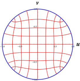
Figure 1: (color online) Unit circle obtained from the conformal map of the square of side $2$.

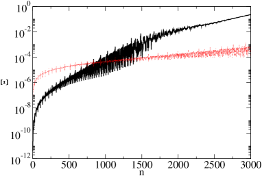
Figure 2: (color online) Error over the first $3000$ energy levels of the circular membrane of radius $r=1$ obtained using CMM with $N=60$ (thick line) and the CCM with $N=100$ (thin line).

We now consider the application of eq. (35): we may pick the coefficients $c_{n}$ minimizing the expectation value in the equation, thus obtaining a precise upper bound to the energy of the ground state. In Fig. 3 we plot the error over the energy of the ground state calculated variationally. A fixed cutoff $N_{int}=36$ has been used for the internal sums; a varying cutoff $N$ is used to limit the number of ”final” states $\psi_{n}(x)$ used in the calculation (remember that the basis in two dimensions is obtained with the direct product of these states and therefore grows as $N^{2}$).

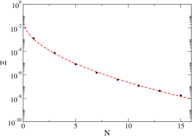
Figure 3: (color online) Error over the energy of the ground state of the circular membrane obtained using eq. (35) and minimizing the coefficients. $N$ is the cutoff in the basis (only the wave functions $\psi_{1}(x)$, $\dots$, $\psi_{N}(x)$ are used). The line is the fit $\Xi_{FIT}=0.058\times 10^{-1.7\sqrt{N}}$.

In Table 3 we display the energies of the twenty lowest levels of the circular membrane obtained using perturbation theory to different orders (up to third order). In the first column we report the quantum numbers corresponding to the states of a square box of side $2$; in the second column we report the degeneracy of the states; in the last column we display the exact results, obtained from the zeroes of the Bessel functions. The formulas obtained in this paper have been applied limiting the internal sum taking $N=20$.

There are several observations that we can make looking at this Table: first, that these results, although perturbative, are rather precise, expecially for the lowest lying states; second, that we are recovering the correct degeneracies observed in the spectrum of the circle: in some cases, such as for the states $(1,2)$ and $(2,1)$ the the interaction term ($\sigma$) is diagonal and therefore the degeneracy is not lifted by perturbation theory; in other cases, such as for the states $(1,3)$ and $(3,1)$ the interaction is not diagonal and therefore perturbation theory splits the levels . However, the lowest of the splitted levels approaches the level corresponding to $(2,2)$, thus approximately reproducing the degeneracy observed in the spectrum of the circle. Finally, for some states we observe level crossing caused by the interaction: this is the case, for example, of the states $(1,5)$ and $(5,1)$, which are splitted by the interaction, yielding a lower state which lyies below the degenerate levels $(3,4)$ and $(4,3)$.

In Fig. 4 we display the energy of the fundamental mode of the unit circle obtained using perturbation theory to order two (triangles) and three (diamonds) as a function of the number of states in the internal sums. The solid line is the exact result, while the dotted line is the result obtained using the simple formula of eq. (40).

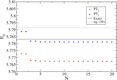
Figure 4: (color online) Energy of the fundamental mode of the unit circle obtained using perturbation theory to order two (triangles) and three (diamonds) as a function of the number of states in the internal sums. The solid line is the exact result. The dotted line is the result of eq. (40).

IV.2 Deformation of the square

We consider the conformal map $f(z)=z+\alpha z^{2}$, for $|\alpha|\ll 1$, which produces a deformation of the square of side $2$. Fig.5 shows the membrane obtained for $\alpha=1/20$.

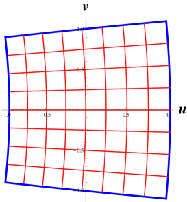
Figure 5: (color online) Deformation of the square of side $2$ produced by the map $f(z)=z+z^{2}/20$.

In this case we have

$$\sigma(x,y) = 4\alpha x+4\alpha^{2}\left(x^{2}+y^{2}\right)\ .$$ (76)

We may easily calculate the matrix elements using the integrals earlier defined:

$$\langle n|\sigma|m\rangle = 4\alpha\mathcal{Q}_{n_{x}m_{x}1}\ \delta_{n_{y}m_{y}}$$ (77)

$$+ 4\alpha^{2}\left(\mathcal{Q}_{n_{x}m_{x}2}\ \delta_{n_{y}m_{y}}+\mathcal{Q}_{n_{y}m_{y}2}\ \delta_{n_{x}m_{x}}\right).$$

In particular:

$$\langle n|\sigma|n\rangle = 4\alpha^{2}\left(\frac{2}{3}-\frac{2}{\pi^{2}n_{x}^{2}}-\frac{2}{\pi^{2}n_{y}^{2}}\right)$$ (78)

for $n=m$ and

$$\langle n|\sigma|m\rangle = \alpha\frac{32m_{x}n_{x}\left((-1)^{m_{x}+n_{x}}-1\right)}{\pi^{2}\left(m_{x}^{2}-n_{x}^{2}\right)^{2}}\ \delta_{n_{y}m_{y}}$$ (79)

$$+ \alpha^{2}\left[\frac{64m_{y}n_{y}\left((-1)^{m_{y}+n_{y}}+1\right)}{\pi^{2}\left(m_{y}^{2}-n_{y}^{2}\right)^{2}}\ \delta_{n_{x}m_{x}}\right.$$

$$+ \left.\frac{64m_{x}n_{x}\left((-1)^{m_{x}+n_{x}}+1\right)}{\pi^{2}\left(m_{x}^{2}-n_{x}^{2}\right)^{2}}\ \delta_{n_{y}m_{y}}\right]$$

for $n\neq m$. Let us discuss explicitly the case of states which are twice degenerate: $|\tilde{n}_{1}\rangle=|n_{x},n_{y}\rangle$ and $|\tilde{n}_{2}\rangle=|n_{y},n_{x}\rangle$ where $n_{x}\neq n_{y}$.

For such states we have that the matrix elements read:

$$\langle\tilde{n}_{1}|\sigma|\tilde{n}_{1}\rangle = \langle\tilde{n}_{2}|\sigma|\tilde{n}_{2}\rangle=\frac{8}{3}\alpha^{2}\left(1-\frac{3}{\pi^{2}n_{x}^{2}}-\frac{3}{\pi^{2}n_{y}^{2}}\right)$$

$$\langle\tilde{n}_{1}|\sigma|\tilde{n}_{2}\rangle = \langle\tilde{n}_{2}|\sigma|\tilde{n}_{1}\rangle=0\ .$$

Since the matrix is diagonal and proportional to the $2\times 2$ identity matrix, the perturbation in this case does not separate the degenerate states and the first order correction in PT is the same as for a the non-degenerate states:

$$E_{n}^{(1)}=-\epsilon_{n}\frac{8}{3}\alpha^{2}\left(1-\frac{3}{\pi^{2}n_{x}^{2}}-\frac{3}{\pi^{2}n_{y}^{2}}\right)\ .$$ (80)

We notice however that $E_{n}^{(1)}$ goes like $\alpha^{2}$, so we need to calculate the $\alpha^{2}$ contribution which comes from the second order correction. As we can see from the matrix elements of $\sigma$ written above, to order $\alpha$ only nondiagonal terms contribute. Therefore, provided that $n_{x}\neq m_{x}$ we have:

$$\langle n|\sigma|m\rangle \approx \alpha\frac{32m_{x}n_{x}\left((-1)^{m_{x}+n_{x}}-1\right)}{\pi^{2}\left(m_{x}^{2}-n_{x}^{2}\right)^{2}}\ \delta_{n_{y}m_{y}}+O\left[\alpha^{2}\right]$$ (81)

We may thus write the contribution to order $\alpha^{2}$ in the second order PT:

$$E_{n}^{(2)} \approx \alpha^{2}\epsilon_{n}^{2}n_{x}^{2}\frac{2^{14}}{\pi^{6}}\ F(n_{x})$$ (82)

where

$$F(n_{x})\equiv\sum_{m_{x}\neq n_{x}}\left[\frac{m_{x}^{2}}{2}\ \frac{\left((-1)^{m_{x}+n_{x}}-1\right)}{\left(n_{x}^{2}-m_{x}^{2}\right)^{5}}\right]\ .$$ (83)

Actually these formulas hold also for states of higher degeneracy, since also in this case the interaction matrix is diagonal and proportional to the identity matrix.

The series appearing in this equation may be calculated analytically (we do not report the expression here because of its length), instead we report the first three values are:

$$F(1) = \frac{\pi^{4}}{3072}-\frac{5\pi^{2}}{1024}\approx-0.0164827$$

$$F(2) = \frac{\pi^{4}}{49152}-\frac{5\pi^{2}}{65536}\approx 0.0012288$$

$$F(3) = \frac{\pi^{4}}{248832}-\frac{5\pi^{2}}{746496}\approx 0.000325359\ .$$

We may also calculate the leading behaviour of $F(n_{x})$ for $n_{x}\rightarrow\infty$. In this case we find:

$$\lim_{n_{x}\rightarrow\infty}F(n_{x})=\frac{\pi^{4}}{3072\ n_{x}^{4}}\approx\frac{0.0317087}{n_{x}^{4}}\ .$$ (84)

Notice that in the limit of highly excited levels, $n_{x}\rightarrow\infty$, we may use the asymptotic behavior of $F(n_{x})$ written above to predict that the energy calculated to order $\alpha^{2}$ behave as

$$E_{n} \approx \epsilon_{n}\left[1+\frac{4}{3}\alpha^{2}\left(\frac{{n_{y}}^{2}+\frac{6}{\pi^{2}}}{{n_{x}}^{2}}+\frac{6}{\pi^{2}{n_{y}}^{2}}-1\right)\right]\ .$$ (85)

Provided that we consider states with $n_{y}\ll n_{x}$ we obtain the following limit

$$E_{n} \approx \epsilon_{n}\left[1-\frac{4}{3}\alpha^{2}\right]$$ (86)

thus being decreased by a constant factor with respect to the energies of the box.

In Table 4 we display the quantity $(E_{n}-E_{n}^{box})/\alpha^{2}$, for different values of $\alpha$ and for the first $50$ states. The energies in the deformed box have been obtained using CCM with $N=60$. In the last column we report the leading perturbative result, corresponding to the analytical formula which has been obtained in this paper. Notice how well the numerical results approach the theoretical one even for moderate values of $\alpha$. Only $15$ of these corrections are positive, the remaining corresponding to a lowering of the frequencies.

Fig. 6 displays the quantity $\Xi\equiv\left|1-\frac{E_{n}^{(CCM)}}{E_{n}^{(PT)}}\right|$ for $\alpha=1/100$ for the first 3000 levels. The numerical CCM results have been obtained with a grid corresponding to $N=100$. The inset plot is the blow-up of the first 200 levels.

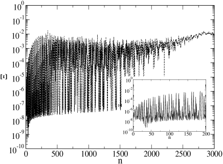
Figure 6: $\Xi\equiv\left|1-\frac{E_{n}^{(CCM)}}{E_{n}^{(PT)}}\right|$ for $\alpha=1/100$ for the first 3000 levels. The numerical CCM results have been obtained with a grid corresponding to $N=100$. The inset plot is the blow-up of the first 200 levels.

In Fig. 7 we display the first $50$ levels of the deformed square as a function of $1/\alpha$. The solid line are the precise numerical results obtained using CCM with $N=60$; the dashed lines are obtained using the analytical formulas that we have obtained.

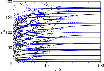
Figure 7: (color online) First 50 levels of the deformed square as a function of $1/\alpha$. The solid lines are the numerical results obtained with CCM with $N=60$; the dashed lines are the analytical perturbative results obtained in this paper.

IV.3 A general formula

Let us therefore consider a general conformal map

$$f(z)=z+\eta\sum_{n=1}^{\infty}\frac{\varrho_{n}}{n}z^{n}\ ,$$ (87)

where $\varrho_{n}$ are real coefficients of similar strength and $\eta$ is a small parameter. Notice that $\varrho_{1}$ is related to a dilatation.

In this case we have

$$\sigma = \eta\sum_{n=2}^{\infty}\varrho_{n}\left((x+iy)^{n-1}+(x-iy)^{n-1}\right)$$

$$+ \eta^{2}\sum_{n,m=2}^{\infty}\varrho_{n}\varrho_{m}(x+iy)^{n-1}(x+iy)^{m-1}$$

$$= \eta\sum_{n=2}^{\infty}\varrho_{n}\sum_{k=0}^{n-1}\ \left(\begin{array}[]{c}n-1\\ k\\ \end{array}\right)\ x^{k}y^{n-1-k}i^{n-1-k}$$

$$\times \left(1+(-1)^{n-1-k}\right)$$

$$+ \eta^{2}\sum_{n,m=2}^{\infty}\varrho_{n}\varrho_{m}(x+iy)^{n-1}(x+iy)^{m-1}\ .$$ (91)

We focus on the term of order $\eta$ and write the corresponding matrix elements

$$\langle n|\sigma|m\rangle \approx \eta\sum_{n=2}^{\infty}\varrho_{n}C_{n;n_{x}m_{x}n_{y}m_{y}}+O\left[\eta^{2}\right]\ ,$$ (92)

where

$$C_{n;n_{x}m_{x}n_{y}m_{y}} \equiv \sum_{k=0}^{n-1}\ \left(\begin{array}[]{c}n-1\\ k\\ \end{array}\right)\ \mathcal{Q}_{n_{x}m_{x}k}\mathcal{Q}_{n_{y}m_{y}n-1-k}$$ (96)

$$i^{n-1-k}\left(1+(-1)^{n-1-k}\right)\ .$$

Notice that an analytical expression for the $C$ is obtained quite easily using the results in the appendix A. In particular the diagonal matrix elements read

$$\langle n|\sigma|n\rangle \approx \eta\left\{\varrho_{3}\ \frac{4\left(\frac{1}{n_{y}^{2}}-\frac{1}{n_{x}^{2}}\right)}{\pi^{2}}+\varrho_{5}\left(\frac{48\left(n_{x}^{4}-n_{x}^{2}n_{y}^{2}+n_{y}^{4}\right)}{\pi^{4}n_{x}^{4}n_{y}^{4}}-\frac{8}{15}\right)\right.$$ (97)

$$- \left.\varrho_{7}\left(\frac{16(n_{x}-n_{y})(n_{x}+n_{y})\left(\pi^{4}n_{x}^{4}n_{y}^{4}-90\left(n_{x}^{4}+n_{y}^{4}\right)\right)}{\pi^{6}n_{x}^{6}n_{y}^{6}}\right)\right.$$

$$+ \left.\varrho_{9}\left(\frac{896\left(90\left(n_{x}^{8}-n_{x}^{6}n_{y}^{2}+n_{x}^{4}n_{y}^{4}-n_{x}^{2}n_{y}^{6}+n_{y}^{8}\right)-\pi^{4}n_{x}^{4}n_{y}^{4}\left(n_{x}^{4}-n_{x}^{2}n_{y}^{2}+n_{y}^{4}\right)\right)}{\pi^{8}n_{x}^{8}n_{y}^{8}}+\frac{32}{45}\right)+\dots\right\}\ .$$

We may now consider the off-diagonal matrix elements between two degenerate states. For the twice degenerate states $|n\rangle=|1,2\rangle$ and $|m\rangle=|2,1\rangle$ we have

$$\langle 12|\sigma|21\rangle = \langle 21|\sigma|12\rangle=0\ .$$ (98)

In this case the degeneration of the levels is not lifted by the perturbation as already discussed earlier. The same occurrs for all the states where $n_{x}$ and $n_{y}$ add to an odd integer.

On the other hand, states where $n_{x}$ and $n_{y}$ add to an even integer do have non vanishing matrix elements. For example, for the states $|n\rangle=|1,3\rangle$ and $|m\rangle=|3,1\rangle$ we have:

$$\langle 13|\sigma|31\rangle = \langle 31|\sigma|13\rangle=-\frac{27\varrho_{5}}{\pi^{4}}+\frac{63\left(8\pi^{4}-765\right)\varrho_{9}}{\pi^{8}}-\frac{297\left(3869775-42840\pi^{4}+32\pi^{8}\right)\varrho_{13}}{2\pi^{12}}$$ (99)

$$+ \frac{135\left(-185977516725+2065943880\pi^{4}-1633632\pi^{8}+256\pi^{12}\right)\varrho_{17}}{\pi^{16}}+\dots$$

For these states the degeneracy is lifted by the perturbation.

In Table 5 we have written the analytical expressions for the first order perturbative corrections (divided by the energy of the square of corresponding quantum numbers and changed of sign) generated by the conformal map written above, for the first $20$ energy levels. The reader may notice that only odd powers in the map contribute to this order. Moreover, the degeneration is lifted only for the states $\left\{|1,3\rangle,|3,1\rangle\right\}$, $\left\{|2,4\rangle,|4,2\rangle\right\}$ and $\left\{|1,5\rangle,|5,1\rangle\right\}$ (for which as mentioned before the sum of the two quantum numbers is even), although the splittings depend only on some of the coefficients ($\varrho_{5}$,$\varrho_{9}$, $\dots$).

IV.4 Robnik’s billiards

Out next application is to Robnik’s billiard, which are obtained using the conformal map of the circle Robnik84

$$f(z) = Az+Bz^{2}\ ,$$ (100)

where $A=\cos p$ and $B=\frac{1}{\sqrt{2}}\sin p$. The parametrization of $A$ and $B$ in terms of $p$ describes a family of billiards of constant area $A=\pi$. We write the map as

$$f(z) = \cos p\ \left[z+\lambda z^{2}\right]\equiv\cos p\ \bar{f}(z)\ .$$ (101)

where we have defined $\lambda\equiv\frac{\tan p}{\sqrt{2}}$ as in Ref. Robnik84 . Since the maps $f(z)$ and $\bar{f}(z)$ are related by a dilatation, one can calculate the eigenvalues corresponding to the second map and easily obtain the eigenvalues corresponding to the first map as:

$$E_{n}=\frac{\bar{E}_{n}}{\cos^{2}p}\ .$$ (102)

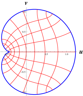
Figure 8: (color online) Robnik’s billiard for $\lambda=1/2$.

We will therefore use the second map and then use the relation above to obtain the eigenvalues corresponding to the first map. We thus have:

$$\Sigma=1+4\lambda r\cos\theta+4\lambda^{2}r^{2}\ ,$$ (103)

and

$$\sigma=4\lambda r\cos\theta+4\lambda^{2}r^{2}\ .$$ (104)

Notice that having chosen to work with the second map rather than with the first one, eliminates a constant term $\sigma$ and therefore simplifies the calculation.

In this case we are working with the orthonormal basis of the circle:

$$\phi_{kns}(r,\theta)\equiv R_{kn}J_{k}(\gamma_{kn}r)\times\left\{\begin{array}[]{cc}\cos k\theta&,\ s=1\\ \sin k\theta&,\ s=2\\ \end{array}\right.$$ (107)

The normalization constants are:

$$R_{0n} = \frac{1}{\sqrt{\pi}\ J_{0}^{\prime}(\gamma_{0n})}\ \ ,\ k=0$$ (108)

$$R_{kn} = \frac{\sqrt{2}}{\sqrt{\pi}\ J_{k}^{\prime}(\gamma_{kn})}\ \ ,\ k>0,$$ (109)

where $J_{k}$ is the Bessel function of order $k$ and $\gamma_{kn}$ its zeroes. We have followed almost entirely the notation of Ref. Robnik84 , apart of introducing an index $s$ for the degeneracy: all states with $k>0$ are twice degenerate, states with $k=0$ are simple.

The application of our perturbative formula requires the calculation of the matrix elements of $\sigma$. Thus we need to calculate:

$$\langle kns|r^{2}|k^{\prime}n^{\prime}s^{\prime}\rangle = \int_{0}^{1}dr\int_{0}^{2\pi}d\phi\ r^{3}\phi_{kns}(r,\theta)\phi_{k^{\prime}n^{\prime}s^{\prime}}(r,\theta)$$ (110)

$$= \pi\left[\delta_{k,k^{\prime}}+(-1)^{s+1}\delta_{k,-k^{\prime}}\right]\delta_{ss^{\prime}}R_{kns}R_{kn^{\prime}s}\int_{0}^{1}drr^{3}J_{k}(\gamma_{kn}r)J_{k}(\gamma_{kn^{\prime}}r)$$

$$\langle kns|r\cos\theta|k^{\prime}n^{\prime}s^{\prime}\rangle = \int_{0}^{1}dr\int_{0}^{2\pi}d\phi\ r^{2}\cos\theta\phi_{kns}(r,\theta)\phi_{k^{\prime}n^{\prime}s^{\prime}}(r,\theta)$$ (111)

$$= g_{kk^{\prime}s}\delta_{ss^{\prime}}R_{kns}R_{k^{\prime}n^{\prime}s}\int_{0}^{1}drr^{2}J_{k}(\gamma_{kn}r)J_{k}(\gamma_{kn^{\prime}}r)$$

where

$$g_{kk^{\prime}s} = \frac{\pi}{2}\ \left[\left(\delta_{k-k^{\prime},1}+\delta_{k-k^{\prime},-1}\right)\right.$$ (112)

$$+ \left.(-1)^{s+1}\left(\delta_{k+k^{\prime},1}+\delta_{k+k^{\prime},-1}\right)\right]\ .$$

Using the integrals above we may obtain the matrix elements of $\sigma$:

$$\langle kns|\sigma|k^{\prime}n^{\prime}s\rangle \equiv \lambda\langle kns|\sigma^{(1)}|k^{\prime}n^{\prime}s\rangle+\lambda^{2}\langle kns|\sigma^{(2)}|k^{\prime}n^{\prime}s\rangle$$ (113)

$$= 4\lambda\langle kns|r\cos\theta|k^{\prime}n^{\prime}s\rangle$$

$$+ 4\lambda^{2}\langle kns|r^{2}|kn^{\prime}s\rangle\ .$$

Notice that the diagonal matrix elements are of order $\lambda^{2}$, whereas the off-diagonal matrix elements start at order $\lambda$. This means that our perturbative (in the power counting parameter $\eta$) formulas contain contributions with different orders in $\lambda$. For example the first order formula is of order $\lambda^{2}$, just as the second order perturbative formula, which contains squares of off-diagonal matrix elements. On the other hand, the third order perturbative formula is of order $\lambda^{4}$, since the last sum, which involves the product of three non-diagonal matrix elements vanishes when the external states are taken to be equal. For this reason, the general results that we have obtained in this paper allow us to make a rigorous perturbative analysis of this problem only to order $\lambda^{2}$.

We may therefore write

$$\bar{E}_{kns}=\bar{E}_{kns}^{(0)}+\lambda^{2}\ \bar{E}_{kns}^{(2)}+O\left[\lambda^{4}\right]$$ (114)

where

$$\bar{E}_{kns}^{(0)} = \gamma_{kn}^{2}$$

$$\bar{E}_{kns}^{(2)} = -\gamma_{kn}^{2}\langle kns|\sigma^{(2)}|kns\rangle+\gamma_{kn}^{4}\sum^{\prime}_{k^{\prime},n^{\prime}}\frac{\langle kns|\sigma^{(1)}|k^{\prime}n^{\prime}s\rangle^{2}}{\gamma_{kn}^{2}-\gamma_{k^{\prime}n^{\prime}}^{2}}$$

and $\sum^{\prime}_{k^{\prime},n^{\prime}}$ means the sum obtained excluding the values $(k^{\prime},n^{\prime})=(k,n)$.

Even before doing any numerical calculation, we may look at the form of the matrix elements of $\sigma$ to understand how the degeneracy of the level of the circle is lifted. We observe that the $s$ dependent component of $g_{k,k^{\prime},s}$ is nonzero only when $(k,k^{\prime})$ is $(0,1)$ or $(1,0)$. This means that only the levels with principal quantum number $k=1$ have the degeneracy lifted. A splitting of the levels corresponding to $k>1$ may only occurr through higher order perturbative contributions (to order $\lambda^{4}$ and higher, and it is therefore highly suppressed.

In Table 6 we display the first $40$ eigenvalues of a Robnik billiard with $\lambda=1/100$ and $\lambda=1/20$, calculated with the perturbative formula (114) to order $\lambda^{0}$ and $\lambda^{2}$ and with the CCM with $N=100$. We may observe that the splitting of the levels corresponding to $k=1$ is reproduced quite well by our formula; in particular the results obtained for $\lambda=1/100$ with second order perturbation theory reproduce amazingly well the numerical CCM results. For $\lambda=1/20$, we observe a small splitting of some of the levels corresponding to $k>1$, such as for example for the states with quantum numbers $(2,1)$. As mentioned before, these splittings come from higher order perturbative corrections, which we are not considering here.

In Fig. 9 we display the splitting of the first two excited levels of the Robnik’s billiard, corresponding to the quantum numbers $(k,n)=(1,1)$, as a function of the parameter $\lambda$. The solid line is the perturbative result to order $\lambda^{2}$, calculated in this paper, which corresponds to $\Delta E^{(PT)}=29.3639418\lambda^{2}+58.7278836\lambda^{4}$ (observe that this expression contains a power $\lambda^{4}$ because of extra power of $\lambda$ coming from the rescaling factor $1/\cos^{2}p$ in the energies); the pluses are the precise numerical results obtained using CCM with $N=100$. Finally, for $\lambda\approx 0.5$, the splitting is seen to behave linearly in $\lambda$: the dashed line represent the linear fit of the last four points, $\Delta E^{(fit)}=0.5095+4.90231\lambda$. A resummation of the perturbative series (assuming that it is possible to calculate it to arbitrary orders), should therefore be able to reproduce this leading asymptotic behaviour. It would also be interesting to study the radius of convergence of the perturbative series and see if it has any relation with the insurgence of quantum chaos.

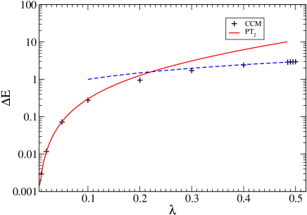
Figure 9: (color online) Splitting of the levels corresponding to $(k,n)=(1,1)$. The solid line is the perturbative result to order $\lambda^{2}$; the pluses are the numerical results obtained with CCM with $N=100$. The dashed line is the linear fit of the four last numerical values $\Delta E^{(fit)}=0.5095+4.90231\lambda$.

IV.5 Regular polygonal billiard

Another interesting application of the techniques discussed in this paper is to the calculation of the frequencies of a regular polygonal billiard. This problem has been attacked in a series of papers, using both numerical and analytical approaches.

In ref. Liboff94 Liboff has studied the polygonal quantum billiard problem, proving that the first excited state of a regular polygon is doubly degenerate. In ref. Liboff01a Liboff and Greenberg have studied the hexagon quantum billiard, constructing a subset of eigenfunctions and eigenvalues, while in ref. Liboff01b Liboff has considered classical and quantum wedge billiards.

Molinari has obtained analytical expressions for the frequency of the ground and first excited states using a perturbative approach, which he calls ”lambda expansion” Molinari97 . Cureton and Kuttler Kuttler99 have used a numerical approach (which is essentially the Conformal Mapping Method of Robnik84 ), to obtain quite precise values for selected eigenvalues of regular polygons and of the figures obtained by the dissection. More recently, Grinfield and Strang Grinfield04 have obtained an analytical formula for the simple states of regular polygonal with ${\cal N}$ sides as a function of $1/{\cal N}$.

Other works have considered specific polygons, and applied different methods to solve the Helmholtz equation on these domains: for example, Betcke and Trefethen have applied the method of particular solutions in ref. Betcke05 to obtain very precise values for the first three eigenvalues of a regular decagon; Lijnen, Chibotaru and Ceulemans, used a radial rescaling approach in ref. Lijnen08 to obtain the ten lowest eigenvalues of regular polygons with ${\cal N}=3,\dots,6$ sides; finally, Guidotti and Lambers Guidotti08 have considered a variant of the method of particular solution, and applied to a regular polygon with $128$ sides (comparing their findings with those predicted by the formula of Grinfield and Strang).

We will now treat this problem with the systematic perturbative approach developed in this paper and then perform a comparison with the works mentioned above.

Our starting point is the conformal map

$$f(z)=C_{\cal N}\int_{0}^{z}\frac{ds}{(1-s^{\cal N})^{2/{\cal N}}}\ ,$$ (115)

which maps the unit circle into a regular polygon of $N$ sides inscribed in the circle Molinari97 ; Kuttler99 . Following Molinari we have defined $C_{\cal N}\equiv\frac{\Gamma(1-1/{\cal N})}{\Gamma(1+1/{\cal N})\Gamma(1-2/{\cal N})}$ and we have expanded the map as

$$f(z)=C_{\cal N}\sum_{k=0}^{\infty}f_{k}z^{{\cal N}k+1}$$ (116)

where $f_{0}=1$ and

$$f_{k}=\frac{1}{k!({\cal N}k+1)}\ \prod_{j=0}^{k-1}\left(\frac{2}{\cal N}+j\right)$$ (117)

for $k\geq 1$.

As explained in the previous section, it is convenient to work with a rescaled map defined through the relation $f(z)\equiv C_{\cal N}\bar{f}(z)$ and then easily relate the eigenvalues corresponding to the map $\bar{f}(z)$ to those corresponding to the map $f(z)$ by means of the equation

$$E_{n}=\frac{\bar{E}_{n}}{C_{\cal N}^{2}}\ .$$ (118)

We thus obtain

$$\Sigma = \sum_{k=0}^{\infty}\sum_{j=0}^{\infty}({\cal N}k+1)({\cal N}j+1)f_{k}f_{j}r^{{\cal N}(k+j)}e^{i{\cal N}(k-j)\theta}$$

and

$$\sigma = -1+\sum_{k=0}^{\infty}\sum_{j=0}^{\infty}({\cal N}k+1)({\cal N}j+1)f_{k}f_{j}r^{{\cal N}(k+j)}e^{i{\cal N}(k-j)\theta}\ .$$

Let us calculate explicitly the matrix elements $\langle kns|\sigma|k^{\prime}n^{\prime}s\rangle$. We define

$${\cal I}^{(1)}_{k,k^{\prime},l,m} \equiv \int_{0}^{2\pi}\cos k\theta\ \cos k^{\prime}\theta\ \cos{\cal N}(l-m)\theta\ d\theta$$ (119)

$$= \frac{\pi}{2}\left[\delta_{k-k^{\prime}+{\cal N}(l-m)}+\delta_{k+k^{\prime}+{\cal N}(l-m)}\right.$$

$$+ \left.\delta_{k-k^{\prime}-{\cal N}(l-m)}+\delta_{k+k^{\prime}-{\cal N}(l-m)}\right]$$

$${\cal I}^{(2)}_{k,k^{\prime},l,m} \equiv \int_{0}^{2\pi}\sin k\theta\ \sin k^{\prime}\theta\ \cos{\cal N}(l-m)\theta\ d\theta$$ (120)

$$= \frac{\pi}{2}\left[\delta_{k-k^{\prime}+{\cal N}(l-m)}-\delta_{k+k^{\prime}+{\cal N}(l-m)}\right.$$

$$+ \left.\delta_{k-k^{\prime}-{\cal N}(l-m)}-\delta_{k+k^{\prime}-{\cal N}(l-m)}\right]$$

which can be written as

$${\cal I}^{(s)}_{k,k^{\prime},l,m} \equiv {\cal I}^{(a)}_{k,k^{\prime},l,m}+(-1)^{s+1}{\cal I}^{(b)}_{k,k^{\prime},l,m}$$

$$= \frac{\pi}{2}\left[\delta_{k-k^{\prime}+{\cal N}(l-m)}+\delta_{k-k^{\prime}-{\cal N}(l-m)}\right]$$

$$+ (-1)^{s+1}\frac{\pi}{2}\left[\delta_{k+k^{\prime}+{\cal N}(l-m)}+\delta_{k+k^{\prime}-{\cal N}(l-m)}\right]\ .$$

We also define

$${\cal J}_{kn,k^{\prime}n^{\prime},{\cal N},l,m}\equiv\int_{0}^{1}r^{{\cal N}(l+m)+1}J_{k}(\gamma_{kn}r)J_{k^{\prime}}(\gamma_{k^{\prime}n^{\prime}}r)dr$$

and thus we may write the matrix element of $\sigma$ as:

$$\langle kns|\sigma|k^{\prime}n^{\prime}s^{\prime}\rangle = -\delta_{kk^{\prime}}\delta_{nn^{\prime}}\delta_{ss^{\prime}}+\sum_{l=0}^{\infty}\sum_{m=0}^{\infty}({\cal N}l+1)({\cal N}m+1)f_{l}f_{m}R_{kn}R_{k^{\prime}n^{\prime}}\delta_{ss^{\prime}}{\cal I}^{(s)}_{k,k^{\prime},l,m}{\cal J}_{kn,k^{\prime}n^{\prime},{\cal N},l,m}\ .$$ (121)

We focus here on the calculation of the first order correction to the eigenvalues:

$$\bar{E}_{kns}^{(1)} = -\gamma_{kn}^{2}\langle kns|\sigma|kns\rangle\ .$$ (122)

We may now explicitly write the diagonal matrix element of $\sigma$:

$$\langle kns|\sigma|kns\rangle = \sum_{l=1}^{\infty}({\cal N}l+1)^{2}f_{l}^{2}R_{kn}^{2}{\cal I}^{(a)}_{k,k,l,l}{\cal J}_{kn,kn,{\cal N},l,l}$$ (123)

$$+ (-1)^{s+1}\sum_{l=0}^{\infty}\sum_{m=0}^{\infty}({\cal N}l+1)({\cal N}m+1)f_{l}f_{m}R_{kn}^{2}{\cal I}^{(b)}_{k,k,l,m}{\cal J}_{kn,kn,{\cal N},l,m}\ ,$$

where the last term, when non-zero, breaks the degeneracy of the states with $s=1$ and $s=2$. If we look at the form of ${\cal I}^{(b)}_{k,k,l,m}$ we see that it does not vanish only when the condition $2k=\pm{\cal N}(l-m)$ is met. We need to distinguish between regular polygons with even or odd numbers of sides: for ${\cal N}$ even, we may fulfill this condition for $k={\cal N}/2$ and $l=m\pm 1$, for $k={\cal N}$ and $l=m\pm 2$, and so on; for ${\cal N}$ odd, this condition is met for $k={\cal N}$ and $l=m\pm 2$, for $k=2{\cal N}$ and $l=m\pm 4$, and so on. Thus, perturbation theory to first order predicts a peculiar pattern of lifting of the degeneracy of levels.

Notice that the radial integrals can also be calculated explicitly:

$${\cal J}_{kn,kn,{\cal N},l,m} = \frac{4^{-k}\gamma_{k,n}^{2k}}{\Gamma(k+1)^{2}(2k+{\cal N}(l+m)+2)}$$

$$\times {}_{2}F_{3}\left(k+\frac{1}{2},k+\frac{l{\cal N}}{2}+\frac{m{\cal N}}{2}+1;k+1,2k+1,k+\frac{l{\cal N}}{2}+\frac{m{\cal N}}{2}+2;-\gamma_{k,n}^{2}\right)\ .$$

We can therefore write the energy calculated up to first order in perturbation theory as

$$E_{kns}=\frac{\gamma_{kn}^{2}}{C_{\cal N}^{2}}\left[1-\langle kns|\sigma|kns\rangle\right]\ .$$ (124)

Let us focus for a moment on the perturbative result obtained at order zero, $E_{kns}\approx\frac{\gamma_{kn}^{2}}{C_{\cal N}^{2}}$. We may expand the factor $1/C_{\cal N}^{2}$ around ${\cal N}=\infty$, obtaining the energies

$$\frac{\gamma_{kn}^{2}}{C_{\cal N}^{2}} \approx \gamma_{kn}^{2}\left[1+\frac{2\pi^{2}}{3{\cal N}^{2}}+\frac{4\zeta(3)}{{\cal N}^{3}}+\frac{14\pi^{4}}{45{\cal N}^{4}}+\dots\right]\ ,$$

which reproduce the formula obtained by Grinfield and Strang in Grinfield04 up to order $1/{\cal N}^{2}$ (notice however that their formula is limited to the simple states). The coefficient of order $1/{\cal N}^{3}$ is different, although very similar numerically: we obtain $4\zeta(3)\approx 4.81$, while ref.Grinfield04 quotes $\pi^{3}/6\approx 5.2$ . On the other hand, if we look now at the first order correction, we clearly see that it is not analytical at ${\cal N}=\infty$ and therefore that it cannot be expanded in powers of $1/{\cal N}$.

In Fig. 10, 11 and 12 we have plotted the first $40$ levels of the octagon, nonagon and decagon billiards, obtained using zero and first order perturbation theory (circles and triangle respectively) and using CCM with a grid corresponding to $N=100$ (pluses). The boxes in the plots enclose the levels where first order PT predicts that degeneracy is lifted: as we have already discussed before, this occurrs at $k={\cal N}/2$ (and multiple integers) for regular polygons with even number of sides ${\cal N}$ and at $k={\cal N}$ (and multiple integers) for regular polygons with odd number of sides. The numerical values corresponding to these plots are reported in Table 7: we like to underline that in some cases the CCM may provide tiny splittings for states which are degenerate. This occurrs because the discretization may explicitly break the symmetry of the billiard, although this splitting is bound to decrease as the grid gets finer and finer. Taking into account this fact, and looking at the Table we may speculate that the states lying below the $({\cal N}/2,1)$ states for even billiards and $({\cal N},1)$ for odd billiards are degenerate (remember that Liboff’s theorem of ref. Liboff94 tells us that the first excited state of the regular polygonal billiard is degenerate). A rigorous proof of this conjecture would require the calculation of higher order perturbative contributions, which we plan to consider in the future.

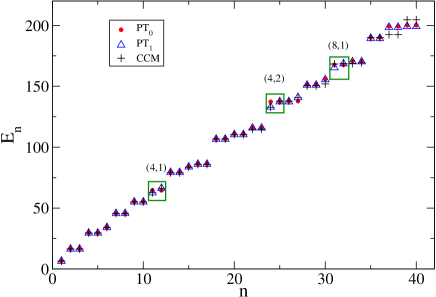
Figure 10: (color online) First 40 levels of a octagon billiard. The circles (triangles) are the results obtained with zero (first) order perturbation theory; the pluses are the exact (numerical) results obtained using CCM with $N=100$. The boxes enclose the levels where first order perturbation theory predicts that the degeneracy of levels is lifted. The corresponding quantum numbers are displayed.

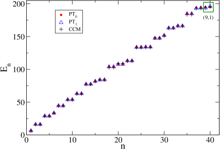
Figure 11: (color online) Same as for Fig. 10 for the nonagon billiard.

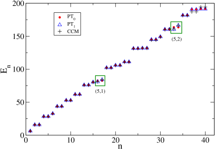
Figure 12: (color online) Same as for Fig. 10 for the decagon billiard.

IV.6 Hamiltonians with position dependent effective mass

As we have mentioned in section III.1, the symmetrized form of the density dependent negative Laplacian operator that we have proposed in this paper had already been introduced in a paper by Zhu and Kroemer, ref. Zhu83 , discussing a different problem.

In recent years there has been lot of interest in discussing the solutions of quantum mechanical models containing density dependent effective masses, which are common in the description of condensed matter systems. However most of the efforts have been put into constructing exactly and quasi-exactly solvable potentials for the Schrödinger equation with position dependent mass terms PDEM . To the best of our knowledge perturbation theory has not been used as a tool to construct the solutions to this problem; since the results obtained earlier in our paper apply straightforwardly to the present case we now extend the approach of section III.2 to Hamiltonians of the form:

$$\hat{H}=\frac{1}{\sqrt{\Sigma}}\left(-\frac{\hbar^{2}}{2m}\hat{\Delta}\right)\frac{1}{\sqrt{\Sigma}}+V\ .$$ (125)

Notice that the stationary Schrödinger equation associated to this operator may be solved numerical using the CCM of section II.2, with the difference that now $\Sigma$ is a physical density, not related to a conformal mapping. Moreover, the matrix representing the operator $\hat{H}$ on the uniform grid, now contains also a diagonal term corresponding to the discretization of the potential $V$. For problems defined on whole space, a suitable strategy corresponds to solve the SSE in a $d$-dimensional cube ($d$ being the dimension of the problem), whose dimensions have been determined variationally, as done in refs. Amore07 ; Amore09b . The only difference in this case is the presence of the spatially dependent density $\Sigma$.

An alternative way of solving the problem consists of resorting to perturbation theory. We may cast this hamiltonian into the form

$$\hat{H}=\frac{1}{\sqrt{\Sigma}}\left(-\frac{\hbar^{2}}{2m}\hat{\Delta}+V_{0}\right)\frac{1}{\sqrt{\Sigma}}+\left(V-\frac{V_{0}}{\Sigma}\right)\ ,$$ (126)

where $V_{0}$ is a potential for which the ”unperturbed” Hamiltonian $\hat{H}_{0}=\left(-\frac{\hbar^{2}}{2m}\hat{\Delta}+V_{0}\right)$ is exactly solvable. The analysis carried out in section III.2 may now be easily generalized, by expressing $\Sigma=1+\eta\sigma$ as before and letting $\left(V-\frac{V_{0}}{\Sigma}\right)\rightarrow\eta\left(V-\frac{V_{0}}{1+\eta\sigma}\right)$. Thus we have

$$\hat{H}=\hat{H}_{0}+\eta\hat{H}_{1}+\eta^{2}\hat{H}_{2}+\eta^{3}\hat{H}_{3}+\dots$$ (127)

where

$$\hat{H}_{1} \equiv \hat{H}_{1}^{(a)}+\hat{H}_{1}^{(b)}$$ (128)

$$= -\frac{1}{2}\left[\sigma\hat{H}_{0}+\hat{H}_{0}\sigma\right]+V-V_{0}$$

$$\hat{H}_{2} \equiv \hat{H}_{2}^{(a)}+\hat{H}_{2}^{(b)}$$ (129)

$$= \frac{1}{8}\left[2\sigma\hat{H}_{0}\sigma+3\sigma^{2}\hat{H}_{0}+3\hat{H}_{0}\sigma^{2}\right]+V_{0}\sigma$$

$$\hat{H}_{3} \equiv \hat{H}_{3}^{(a)}+\hat{H}_{3}^{(b)}$$ (130)

$$= -\frac{3}{16}\left[\sigma^{2}\hat{H}_{0}\sigma+\sigma\hat{H}_{0}\sigma^{2}\right]-\frac{5}{16}\left[\sigma^{3}\hat{H}_{0}+\hat{H}_{0}\sigma^{3}\right]$$

$$- V_{0}\sigma^{2}\ ,$$

where the operators $\hat{H}_{i}^{(a)}$ are those which contain $\hat{H}_{0}$ and are equivalent to the one obtained before. Working up to second order and calling $\epsilon_{n}$ and $|n\rangle$ the eigenenergies and eigenstates of $\hat{H}_{0}$ we find

$$E_{n}^{(1)} = -\epsilon_{n}\langle n|\sigma|n\rangle+\langle n|V-V_{0}|n\rangle$$ (131)

$$E_{n}^{(2)} = \epsilon_{n}\langle n|\sigma|n\rangle^{2}+\epsilon_{n}^{2}\sum_{k\neq n}\frac{\langle n|\sigma|k\rangle^{2}}{\epsilon_{n}-\epsilon_{k}}$$ (132)

$$+ 2\sum_{k\neq n}\frac{\langle n|\hat{H}_{1}^{(a)}|k\rangle\langle k|\hat{H}_{1}^{(b)}|n\rangle}{\epsilon_{n}-\epsilon_{k}}$$

$$+ \sum_{k\neq n}\frac{\langle n|\hat{H}_{1}^{(b)}|k\rangle^{2}}{\epsilon_{n}-\epsilon_{k}}\ .$$

Let us consider the term:

$$E_{n}^{(2b)} \equiv 2\sum_{k\neq n}\frac{\langle n|\hat{H}_{1}^{(a)}|k\rangle\langle k|\hat{H}_{1}^{(b)}|n\rangle}{\epsilon_{n}-\epsilon_{k}}$$ (133)

$$= -\sum_{k\neq n}\frac{\epsilon_{n}+\epsilon_{k}}{\epsilon_{n}-\epsilon_{k}}\langle n|\sigma|k\rangle\langle k|V-V_{0}|n\rangle$$

$$= -\left(\langle n|\sigma(V-V_{0})|n\rangle-\langle n|\sigma|n\rangle\langle n|V-V_{0}|n\rangle\right)$$

$$- 2\sum_{k\neq n}\frac{\epsilon_{k}}{\epsilon_{n}-\epsilon_{k}}\langle n|\sigma|k\rangle\langle k|V-V_{0}|n\rangle\ .$$

Therefore we have

$$E_{n}^{(2)} = \epsilon_{n}\langle n|\sigma|n\rangle^{2}+\epsilon_{n}^{2}\sum_{k\neq n}\frac{\langle n|\sigma|k\rangle^{2}}{\epsilon_{n}-\epsilon_{k}}$$ (134)

$$- \left(\langle n|\sigma(V-V_{0})|n\rangle-\langle n|\sigma|n\rangle\langle n|V-V_{0}|n\rangle\right)$$

$$- 2\sum_{k\neq n}\frac{\epsilon_{k}}{\epsilon_{n}-\epsilon_{k}}\langle n|\sigma|k\rangle\langle k|V-V_{0}|n\rangle$$

$$+ \sum_{k\neq n}\frac{\langle n|V-V_{0}|k\rangle^{2}}{\epsilon_{n}-\epsilon_{k}}\ .$$

Likewise we may find the perturbative corrections to the eigenstates of the Hamiltonian; for example, we may consider the special case where $V=V_{0}/\sqrt{\Sigma}$, and therefore obtain to first order in perturbation theory:

$$|\Psi_{n}\rangle=|n\rangle-\frac{\eta}{2}\sum_{k\neq n}\frac{\epsilon_{n}+\epsilon_{k}}{\epsilon_{n}-\epsilon_{k}}|k\rangle\langle k|\sigma|n\rangle+\dots$$ (135)

We may apply this expression to the calculation of the uncertainties over position and momentum:

$$\Delta x_{n} \approx \Delta x_{n}^{(0)}\ \left(1-\frac{\eta}{2}\sum_{k\neq n}\frac{\epsilon_{n}+\epsilon_{k}}{\epsilon_{n}-\epsilon_{k}}\frac{\langle k|\sigma|n\rangle}{\left(\Delta x_{n}^{(0)}\right)^{2}}\right.$$ (136)

$$\times \left.\left(\langle n|x^{2}|k\rangle-\langle n|x|n\rangle\langle n|x|k\rangle\right)\right)$$

$$\Delta p_{n} \approx \Delta p_{n}^{(0)}\ \left(1-\frac{\eta}{2}\sum_{k\neq n}\frac{\epsilon_{n}+\epsilon_{k}}{\epsilon_{n}-\epsilon_{k}}\frac{\langle k|\sigma|n\rangle}{\left(\Delta p_{n}^{(0)}\right)^{2}}\right.$$ (137)

$$\times \left.\left(\langle n|p^{2}|k\rangle-\langle n|p|n\rangle\langle n|p|k\rangle\right)\right)\ .$$

We thus obtain the product of the uncertainties

$$\Delta x_{n}\Delta p_{n} \approx \Delta x_{n}^{(0)}\Delta p_{n}^{(0)}\ \left[1-\frac{\eta}{2}\sum_{k\neq n}\frac{\epsilon_{n}+\epsilon_{k}}{\epsilon_{n}-\epsilon_{k}}\langle k|\sigma|n\rangle\right.$$ (138)

$$\times \left.\left(\frac{\left(\langle n|x^{2}|k\rangle-\langle n|x|n\rangle\langle n|x|k\rangle\right)}{\left(\Delta x_{n}^{(0)}\right)^{2}}+\frac{\left(\langle n|p^{2}|k\rangle-\langle n|p|n\rangle\langle n|p|k\rangle\right)}{\left(\Delta p_{n}^{(0)}\right)^{2}}\right)+O\left[\eta^{2}\right]\right]\ ,$$

which for the simple harmonic oscillator simplifies to

$$\Delta x_{n}\Delta p_{n} \approx \Delta x_{n}^{(0)}\Delta p_{n}^{(0)}\ \left(1+O\left[\eta^{2}\right]\right)\ .$$ (139)

V Conclusions

Our paper contains strong numerical and analytical results for the solution of the Helmholtz equation on general domains. We briefly state the novelties and advantages of the approaches outlined in this work:

• The extension of the CMM of Robnik Robnik84 to use the orthonormal basis of a square allows to express the integrals (for polynomial conformal mapping or mapping which can be well approximated by polynomials) analytically. This clearly reduces the computation times and improves the precision.

• The computational advantages of the CCM of Amore Amore08 are made clear: the collocation matrix is made of two parts, a ”universal” matrix, corresponding to the discretization of the negative Laplacian, which can be calculated once and for all for a given grid, and a specific ”shape dependent” matrix, which is diagonal and therefore may be calculated quite efficiently. In this approach no integrals are ever needed to be calculated.

• We prove two theorems which provide explicit formulas for the ground and excited states of a quantum billiard. These theorems essentially implement the very well known ”power method” for finite dimensional matrices, to operators in an infinite dimensional Hilbert space. The variational theorem also allows to obtain upper bounds to the ground state energy.

• We have formulated a systematic perturbation theory for membranes obtained slightly deforming a square or circular membrane. Our perturbation scheme is essentially the Rayleigh-Schrödinger perturbation theory with a specific form of the interaction operator. The perturbative results discussed in this paper are in most cases very precise and provide a clear and simple explanation of the mechanism responsible for the lifting of degeneracies. For the case of the small deformations of the square, we have obtained an analytical formula for the whole spectrum. A possible application of our shape perturbation theory could be to the calculation of Casimir energies due to deformations of membranes. In a recent interesting paper, ref. Mazzitelli09 , for example, the point matching method has been used to numerically calculate Casimir energies for perfect-conductor waveguide of arbitrary section. Our perturbative approach could be useful for analytical calculations.

• The shape perturbation theory of the present paper could be applied to study the statistical distribution of the energy level spacings for quantum billiards obtained from small perturbations of the square or of the circle. In this case the study would provide an alternative tool to purely numerical methods or to asymptotic methods.

• We have provided a way to extract (at least in principle) the perturbative coefficients of the energy of a given level to a specific order. It would be certainly interesting to study the convergence properties of the perturbative series corresponding to quantum billiards of different shape and see if a relation between the chaotic behaviour of a billiard and the perturbative series could be established.

• The analytical results contained in the paper are not limited to two dimensional membranes, but can be used for problems of higher dimensions; moreover they can also be applied to describe the spectrum of arbitrary inhomogeneous membranes. A numerical study of this problem using the CCM has been already performed in Amore09 ; we plan to look at this problem with the analytical techniques of the present paper in the near future. Here we have applied our results to Hamiltonians containing position dependent effective masses, extending the perturbative approach developed for the Helmholtz equation.

We believe that several developments may stem out of the results contained in this paper: among these, it would certainly be worth looking at possible non-perturbative extensions of our shape perturbation method, which we plan to look at in the near future. Similarly, we plan to carry out an extension of the perturbative calculation of this paper to higher orders. A further interesting application could be to the inverse problem: in a classical paper, Kac  Kac66 posed the question whether one can hear the sound of a drum, meaning by this if the complete knowledge of the spectrum of a drum is sufficient to determine its shape. We now know that the answer to this question is negative, since in 1992 Gordon, Webb and Wolpert  Gordon92 found an example of two two-dimensional not isometric drums which are isospectral. On the other hand, the perturbative formulas obtained in this paper might be used to find the shape of a drum which is obtained from a small deformation of a square or of a circle, knowing a number of frequencies. Finally the last application that we wish to mention is to the vibration of drums with fractal boundaries: refs.Lapidus95 ; Neuberger06 ; Banjai07 , for example, consider the vibration of a membrane whose border is the Koch snowflake. In particular Banjai Banjai07 uses a conformal transformation to map the snowflake into the unit circle and then performs a spectral collocation to obtain numerical results. Our perturbative approach, given the conformal map, is directly applicable to this problem and could maybe provide further insight in this problem.

Appendix A Recurrence relations

We introduce the definitions:

$$\phi_{n}(x) \equiv \sin\left(\frac{n\pi}{2}(x+1)\right)$$ (140)

$$\chi_{n}(x) \equiv \frac{\delta_{n0}}{\sqrt{2}}+\theta(n-1)\cos\left(\frac{n\pi}{2}(x+1)\right)\ ,$$ (141)

where $\theta(n-1)=1$ for $n\geq 1$.

Notice that these functions obey Dirichlet and von Neumann boundary conditions respectively and that they are orthonormal:

$$\int_{-1}^{+1}\phi_{n}(x)\phi_{m}(x)dx=\int_{-1}^{+1}\chi_{n}(x)\chi_{m}(x)dx=\delta_{nm}\ .$$ (142)

We consider the integrals:

$$\mathcal{Q}_{nmk} \equiv \int_{-1}^{+1}dx\ x^{k}\ \phi_{n}(x)\phi_{m}(x)$$ (143)

$$\mathcal{R}_{nmk} \equiv \int_{-1}^{+1}dx\ x^{k}\ \chi_{n}(x)\chi_{m}(x)\ .$$ (144)

With simple algebra we are able to obtain recurrence relations. First we consider the case $m\neq n$:

$$\mathcal{Q}_{nmk} = -\frac{m^{2}+n^{2}}{(k+1)(k+2)}\frac{\pi^{2}}{4}\mathcal{Q}_{nmk+2}$$ (145)

$$+ \frac{mn}{(k+1)(k+2)}\frac{\pi^{2}}{2}\mathcal{R}_{nmk+2}$$

$$\mathcal{R}_{nmk} = \frac{(-1)^{k}+(-1)^{m+n}}{k+1}-\frac{m^{2}+n^{2}}{(k+1)(k+2)}\frac{\pi^{2}}{4}\mathcal{R}_{nmk+2}$$ (146)

$$+ \frac{mn}{(k+1)(k+2)}\frac{\pi^{2}}{2}\mathcal{Q}_{nmk+2}\ .$$

These equations may be solved to yield the recurrence relations:

$$\mathcal{Q}_{nmk+2} = \frac{8(k+2)mn\left((-1)^{k}+(-1)^{m+n}\right)}{\pi^{2}\left(m^{2}-n^{2}\right)^{2}}$$ (147)

$$- \frac{4(k+1)(k+2)\left(m^{2}+n^{2}\right)}{\pi^{2}\left(m^{2}-n^{2}\right)^{2}}\mathcal{Q}_{nmk}$$

$$- \frac{8(k+1)(k+2)mn}{\pi^{2}\left(m^{2}-n^{2}\right)^{2}}\mathcal{R}_{nmk}$$

$$\mathcal{R}_{nmk+2} = \frac{4(k+2)\left(m^{2}+n^{2}\right)\left((-1)^{k}+(-1)^{m+n}\right)}{\pi^{2}\left(m^{2}-n^{2}\right)^{2}}$$ (148)

$$- \frac{8(k+1)(k+2)mn}{\pi^{2}\left(m^{2}-n^{2}\right)^{2}}\mathcal{Q}_{nmk}$$

$$- \frac{4(k+1)(k+2)\left(m^{2}+n^{2}\right)}{\pi^{2}\left(m^{2}-n^{2}\right)^{2}}\mathcal{R}_{nmk}$$

For $m=n$ we have

$$\mathcal{Q}_{nmk}+\mathcal{R}_{nmk}=\frac{1+(-1)^{k}}{k+1}$$ (149)

and

$$\mathcal{Q}_{nmk} = \frac{\pi^{2}\left((-1)^{k}+1\right)n^{2}}{2\left(k^{3}+6k^{2}+11k+6\right)}$$ (150)

$$- \frac{\pi^{2}n^{2}}{k^{2}+3k+2}\mathcal{Q}_{nmk+2}$$

which is easily solved to give

$$\mathcal{Q}_{nmk+2} = \frac{(-1)^{k}+1}{2(k+3)}-\frac{k^{2}+3k+2}{\pi^{2}n^{2}}\ \mathcal{Q}_{nmk}\ .$$ (151)

After calculating explicitly $\mathcal{Q}_{nm0}$, $\mathcal{Q}_{nm1}$, $\mathcal{R}_{nm0}$ and $\mathcal{R}_{nm1}$ one may then obtain the coefficients of higher order by simply applying the recurrence relations.

For instance:

$$\mathcal{Q}_{nm0} = \delta_{nm}$$

$$\mathcal{Q}_{nn1} = 0\ ,\ m=n$$

$$\mathcal{Q}_{nm1} = \frac{8mn\left((-1)^{m+n}-1\right)}{\pi^{2}\left(m^{2}-n^{2}\right)^{2}}\ ,\ m\neq n$$

$$\mathcal{Q}_{nn2} = \frac{1}{3}-\frac{2}{\pi^{2}n^{2}}\ ,\ m=n$$

$$\mathcal{Q}_{nm2} = \frac{16mn\left((-1)^{m+n}+1\right)}{\pi^{2}\left(m^{2}-n^{2}\right)^{2}}\ ,\ m=n$$

$$\mathcal{Q}_{nn3} = 0\ ,\ m=n$$

$$\mathcal{Q}_{nm3} = \frac{24mn\left((-1)^{m+n}-1\right)}{\pi^{4}\left(m^{2}-n^{2}\right)^{4}}$$

$$\times \left(\pi^{2}\left(m^{2}-n^{2}\right)^{2}-16\left(m^{2}+n^{2}\right)\right)\ ,\ m\neq n$$

$$\dots$$

Appendix B Perturbation theory

In this section we give some detail on the calculation of the perturbative coefficients for the energy. In the following we introduce the definition $\omega_{nk}\equiv\epsilon_{n}-\epsilon_{k}$. We may use the expressions given in eqns.(48),(49),(50) and (51) inside the general formulas of eqns.(52),(53),(54) and (55) to obtain the analytical expressions which are reported in the paper.

We start with the second order term, since the zero and first order terms are straightforward. In this case we obtain:

$$E_{n}^{(2)} = \frac{1}{4}\left[\sum_{l}\langle n|\sigma|l\rangle\epsilon_{l}+3\epsilon_{n}\langle n|\sigma^{2}|n\rangle\right]$$ (152)

$$+ \frac{1}{4}\sum_{k\neq n}\frac{\langle n|\sigma|k\rangle^{2}}{\omega_{nk}}(\epsilon_{n}+\epsilon_{k})^{2}$$

Notice that the first sum in this expression is unrestricted, since $l$ can take all possible value, including $l=n$. It is convenient to express the unrestricted sums isolating the term corresponding to $l=n$, i.e. writing $\sum_{l}f(l)=f(n)+\sum_{l\neq n}f(l)$.

Keeping in mind this observation we may rewrite the first term of the equation above as

$$\left.E_{n}^{(2)}\right|_{I} = \frac{1}{4}\left[\sum_{l}\langle n|\sigma|l\rangle\epsilon_{l}+3\epsilon_{n}\langle n|\sigma^{2}|n\rangle\right]$$

$$= \frac{3}{4}\epsilon_{n}\langle n|\sigma^{2}|n\rangle+\frac{1}{4}\epsilon_{n}\langle n|\sigma|n\rangle^{2}+\frac{1}{4}\sum_{k\neq n}\langle n|\sigma|k\rangle^{2}\epsilon_{k}\ .$$

Similarly we may simplify the second term:

$$\left.E_{n}^{(2)}\right|_{II} = \frac{1}{4}\sum_{k\neq n}\frac{\langle n|\sigma|k\rangle^{2}}{\omega_{nk}}(\epsilon_{n}+\epsilon_{k})^{2}$$

$$= \epsilon_{n}^{2}\sum_{k\neq n}\frac{\langle n|\sigma|k\rangle^{2}}{\omega_{nk}}$$

$$- \epsilon_{n}\sum_{k\neq n}\langle n|\sigma|k\rangle^{2}+\frac{1}{4}\sum_{k\neq n}\langle n|\sigma|k\rangle^{2}\omega_{nk}$$

$$= \epsilon_{n}^{2}\sum_{k\neq n}\frac{\langle n|\sigma|k\rangle^{2}}{\omega_{nk}}-\epsilon_{n}\left(\langle n|\sigma^{2}|n\rangle-\langle n|\sigma|n\rangle^{2}\right)$$

$$+ \frac{\epsilon_{n}}{4}\left(\langle n|\sigma^{2}|n\rangle-\langle n|\sigma|n\rangle^{2}\right)-\frac{1}{4}\sum_{k\neq n}\langle n|\sigma|k\rangle^{2}\epsilon_{k}\ .$$

Combining the two terms we obtain the final result:

$$E_{n}^{(2)}=\epsilon_{n}\langle n|\sigma|n\rangle^{2}+\epsilon_{n}^{2}\sum_{k\neq n}\frac{\langle n|\sigma|k\rangle^{2}}{\epsilon_{n}-\epsilon_{k}}\ .$$ (153)

The third order contribution reads:

$$E_{n}^{(3)} = \frac{3}{8}\sum_{l}\omega_{nl}\langle n|\sigma^{2}|l\rangle\langle l|\sigma|n\rangle-\epsilon_{n}\langle n|\sigma^{3}|n\rangle-\frac{3}{8}\sum_{k\neq n}\langle n|\sigma|k\rangle\langle k|\sigma^{2}|n\rangle\frac{(\epsilon_{n}+\epsilon_{k})^{2}}{\omega_{nk}}$$ (154)

$$- \frac{1}{4}\sum_{k\neq n}\sum_{l}\langle n|\sigma|k\rangle\langle k|\sigma|l\rangle\langle l|\sigma|n\rangle\frac{\epsilon_{l}(\epsilon_{n}+\epsilon_{k})}{\omega_{nk}}-\frac{1}{8}\sum_{k\neq n}\sum_{m\neq n}\langle n|\sigma|k\rangle\langle k|\sigma|m\rangle\langle m|\sigma|n\rangle\frac{(\epsilon_{n}+\epsilon_{k})(\epsilon_{n}+\epsilon_{m})(\epsilon_{m}+\epsilon_{k})}{\omega_{nk}\omega_{nm}}$$

$$+ \frac{1}{4}\epsilon_{n}\langle n|\sigma|n\rangle\sum_{k\neq n}\langle n|\sigma|k\rangle^{2}\frac{(\epsilon_{n}+\epsilon_{k})^{2}}{\omega_{nk}^{2}}\ .$$

We may simplify this expression by arranging term with equal number of sums together. Keeping in mind this simple observation we consider the terms in the above expression which contain two sums:

$$\left.E_{n}^{(3)}\right|_{2sums} = -\frac{1}{8}\sum_{k\neq n}\sum_{m\neq n}\langle n|\sigma|k\rangle\langle k|\sigma|m\rangle\langle m|\sigma|n\rangle\left[\frac{\epsilon_{m}(\epsilon_{n}+\epsilon_{k})}{\omega_{nk}}+\frac{\epsilon_{k}(\epsilon_{n}+\epsilon_{m})}{\omega_{nm}}+\frac{(\epsilon_{n}+\epsilon_{k})(\epsilon_{n}+\epsilon_{m})(\epsilon_{m}+\epsilon_{k})}{\omega_{nk}\omega_{nm}}\right]$$ (155)

$$= -\frac{\epsilon_{n}}{4}\sum_{k\neq n}\sum_{m\neq n}\langle n|\sigma|k\rangle\langle k|\sigma|m\rangle\langle m|\sigma|n\rangle\left[2-3\epsilon_{n}\left(\frac{1}{\omega_{nk}}+\frac{1}{\omega_{nm}}\right)+4\frac{\epsilon_{n}^{2}}{\omega_{nk}\omega_{nm}}\right]\ .$$

We start with the first term in the square parenthesis:

$$\left.E_{n}^{(3)}\right|_{2sums}^{I} = -\frac{\epsilon_{n}}{2}\left(\langle n|\sigma^{3}|n\rangle-2\langle n|\sigma^{2}|n\rangle\langle n|\sigma|n\rangle+\langle n|\sigma|n\rangle^{3}\right)\ .$$ (156)

We now come to the second and term terms in the square parethesis: a simple relabeling of the summed indices shows us that these terms are equal and therefore:

$$\left.E_{n}^{(3)}\right|_{2sums}^{II} = \frac{3}{2}\epsilon_{n}^{2}\sum_{k\neq n}\sum_{m\neq n}\frac{\langle n|\sigma|k\rangle\langle k|\sigma|m\rangle\langle m|\sigma|n\rangle}{\omega_{nk}}$$ (157)

$$= \frac{3}{2}\epsilon_{n}^{2}\sum_{k\neq n}\frac{\langle n|\sigma|k\rangle}{\omega_{nk}}\left[\langle k|\sigma^{2}|n\rangle-\langle k|\sigma|n\rangle\langle n|\sigma|n\rangle\right]\ .$$

Finally we write the last term as:

$$\left.E_{n}^{(3)}\right|_{2sums}^{III} = -\epsilon_{n}^{3}\sum_{k\neq n}\sum_{m\neq n}\frac{\langle n|\sigma|k\rangle\langle k|\sigma|m\rangle\langle m|\sigma|n\rangle}{\omega_{nk}\omega_{nm}}$$ (158)

We may now write

$$E_{n}^{(3)} = \frac{3}{8}\sum_{l\neq n}\omega_{nl}\langle n|\sigma^{2}|l\rangle\langle l|\sigma|n\rangle-\epsilon_{n}\langle n|\sigma^{3}|n\rangle-\frac{3}{8}\sum_{k\neq n}\langle n|\sigma|k\rangle\langle k|\sigma^{2}|n\rangle\frac{(\epsilon_{n}+\epsilon_{k})^{2}}{\omega_{nk}}$$ (159)

$$- \frac{1}{4}\sum_{k\neq n}\langle n|\sigma|k\rangle\langle k|\sigma|n\rangle\langle n|\sigma|n\rangle\frac{\epsilon_{n}(\epsilon_{n}+\epsilon_{k})}{\omega_{nk}}+\frac{1}{4}\epsilon_{n}\langle n|\sigma|n\rangle\sum_{k\neq n}\langle n|\sigma|k\rangle^{2}\frac{(\epsilon_{n}+\epsilon_{k})^{2}}{\omega_{nk}^{2}}$$

$$- \frac{\epsilon_{n}}{2}\left(\langle n|\sigma^{3}|n\rangle-2\langle n|\sigma^{2}|n\rangle\langle n|\sigma|n\rangle+\langle n|\sigma|n\rangle^{3}\right)+\frac{3}{2}\epsilon_{n}^{2}\sum_{k\neq n}\frac{\langle n|\sigma|k\rangle}{\omega_{nk}}\left[\langle k|\sigma^{2}|n\rangle-\langle k|\sigma|n\rangle\langle n|\sigma|n\rangle\right]$$

$$- \epsilon_{n}^{3}\sum_{k\neq n}\sum_{m\neq n}\frac{\langle n|\sigma|k\rangle\langle k|\sigma|m\rangle\langle m|\sigma|n\rangle}{\omega_{nk}\omega_{nm}}\ .$$

With simple algebra we obtain:

$$E_{n}^{(3)} = -\epsilon_{n}\langle n|\sigma|n\rangle^{3}+\epsilon_{n}^{3}\langle n|\sigma|n\rangle\sum_{k\neq n}\frac{\langle n|\sigma|k\rangle^{2}}{\omega_{nk}^{2}}-3\epsilon_{n}^{2}\langle n|\sigma|n\rangle\sum_{k\neq n}\frac{\langle n|\sigma|k\rangle^{2}}{\omega_{nk}}$$ (160)

$$- \epsilon_{n}^{3}\sum_{k\neq n}\sum_{m\neq n}\frac{\langle n|\sigma|k\rangle\langle k|\sigma|m\rangle\langle m|\sigma|n\rangle}{\omega_{nk}\omega_{nm}}\ .$$

$N$	$E_{0}$	$E_{1,2}$	$E_{3,4}$
$10$	5.7831903186	14.682015349	26.374703996
$20$	5.7831860077	14.681971199	26.374617574
$30$	5.7831859657	14.681970679	26.374616505
$40$	5.7831859633	14.681970647	26.374616438
$50$	5.7831859630	14.681970643	26.374616430
$60$	5.7831859630	14.681970642	26.374616428
exact	5.7831859629	14.681970642	26.374616427

Table 1: Three lowest energy eigenvalues of a circular membrane of unit radius obtained using the Collocation Mapping Method with different number of elements. The conformal map is approximated with the Taylor series up to order $z^{37}$.

$N$	$E_{0}$	$E_{1,2}$	$E_{3,4}$
$20$	5.7833478471	14.683030231	26.376321659
$40$	5.7831962133	14.682036989	26.374723431
$60$	5.7831879924	14.681983747	26.374637569
$80$	5.7831866056	14.681974789	26.374623117
$100$	5.7831862262	14.681972340	26.374619167
exact	5.7831859629	14.681970642	26.374616427

Table 2: Three lowest energy eigenvalues of a circular membrane of unit radius obtained using the Collocation Collocation Method with different grid size.

$(n_{x},n_{y})$	$d$	PT0	PT1	PT2	PT3	exact
$(1,1)$	1	4.93480	5.66472	5.76740	5.78118	5.78319
$(1,2)$	2	12.3370	14.4197	14.6695	14.6844	14.68197
$(2,1)$		12.3370	14.4197	14.6695	14.6844	14.68197
$(2,2)$	1	19.7392	25.0228	26.1714	26.3593	26.37462
$(1,3)$	2	24.6740	26.4137	26.4007	26.3785	26.37462
$(3,1)$		24.6740	30.2612	30.7573	30.5467	30.47126
$(2,3)$	2	32.0762	40.3174	41.4936	41.1156	40.70647
$(3,2)$		32.0762	40.3174	41.4936	41.1156	40.70647
$(1,4)$	2	41.9458	47.7922	48.5522	48.9791	49.21846
$(4,1)$		41.9458	47.7922	48.5522	48.9791	49.21846
$(3,3)$	1	44.4132	55.1980	57.6642	57.9679	57.58294
$(2,4)$	2	49.3480	57.1883	57.7144	57.6217	57.58294
$(4,2)$		49.3480	66.4508	71.4408	72.0826	70.85000
$(3,4)$	2	61.6850	76.3544	77.2464	76.2107	76.93893
$(4,3)$		61.6850	76.3544	77.2464	76.2107	76.93893
$(1,5)$	2	64.1524	72.9892	71.1717	70.3712	70.85000
$(5,1)$		64.1524	72.5674	73.5746	74.6076	74.88701
$(5,2)$	2	71.5546	89.4650	96.8822	99.3590	95.27757
$(2,5)$		71.5546	89.4650	96.8822	99.3590	95.27757
$(4,4)$	1	78.9568	97.3221	97.4219	96.4281	98.72627

Table 3: Energy of the twenty lowest states of the circular membrane calculated with perturbation theory to different orders.

$n$	$\alpha=\frac{1}{25}$	$\alpha=\frac{1}{50}$	$\alpha=\frac{1}{100}$	$\alpha=\frac{1}{200}$	$\alpha=\frac{1}{400}$	$\alpha=\frac{1}{800}$	PT
1	-11.9314	-11.9828	-11.9957	-11.9989	-11.9997	-11.9999	-12
2	-62.2270	-62.9170	-63.0930	-63.1372	-63.1482	-63.1510	-63.15197799
3	-7.74588	-7.6738	-7.6556	-7.6510	-7.6498	-7.6495	-7.649505501
4	-12.8722	-12.2228	-12.0560	-12.0139	-12.0034	-12.0007	-12
5	-207.2669	-212.6755	-214.1045	-214.4669	-214.5578	-214.5805	-214.5883271
6	-13.27723	-13.2145	-13.1989	-13.1950	-13.1940	-13.1938	-13.19388958
7	-25.0501	-24.8644	-24.8184	-24.8069	-24.8040	-24.8033	-24.80336862
8	3.2132	8.2394	9.5815	9.9228	10.0085	10.0299	10.03674606
9	-529.3273	-558.6905	-567.0588	-569.2278	-569.7751	-569.9123	-569.9586259
10	-22.0706	-21.9810	-21.9587	-21.9531	-21.9517	-21.9513	-21.95180463
11	-12.8590	-12.2085	-12.0512	-12.0123	-12.0026	-12.0002	-12
12	-44.8505	-44.7072	-44.6716	-44.6627	-44.6605	-44.6599	-44.66052201
13	46.7717	74.1811	82.1277	84.1959	84.7183	84.8492	84.89208802
14	-39.7638	-39.5706	-39.5237	-39.5120	-39.5091	-39.5084	-39.50940841
15	30.6629	33.2746	33.8759	34.0227	34.0591	34.0682	34.0699668
16	-1109.8341	-1223.2138	-1259.7952	-1269.6749	-1272.1960	-1272.8294	-1273.042285
17	-33.6433	-33.4920	-33.4543	-33.4449	-33.4425	-33.4419	-33.44310862
18	-70.2925	-70.1087	-70.0628	-70.0513	-70.0484	-70.0477	-70.04918774
19	102.5451	207.3338	242.1806	251.6572	254.0794	254.6883	254.8899234
20	-12.5604	-12.1285	-12.0299	-12.0059	-11.9999	-11.9984	-12
21	-70.6796	-70.5877	-70.5651	-70.5595	-70.5581	-70.5577	-70.55997503
22	124.8295	134.9087	137.0858	137.6039	137.7317	137.7635	137.7717825
23	-2007.8189	-2335.7052	-2460.1854	-2496.0792	-2505.4160	-2507.7742	-2508.565211
24	-47.9136	-47.6534	-47.5887	-47.5725	-47.5685	-47.5675	-47.56994783
25	-101.2945	-101.0139	-100.9438	-100.9262	-100.9219	-100.9208	-100.9237065
26	115.2123	410.2533	528.4606	562.9517	571.9490	574.2230	574.980025
27	-53.7499	-53.6334	-53.6067	-53.6002	-53.5986	-53.5981	-53.60145365
28	50.1431	51.1784	51.3848	51.4331	51.4450	51.4480	51.44555258
29	-106.3989	-106.3559	-106.3450	-106.3423	-106.3416	-106.3414	-106.3455495
30	286.6324	322.1690	329.4268	331.0946	331.5016	331.6027	331.632198
31	-3256.1580	-4011.4680	-4354.9098	-4463.3391	-4492.3946	-4499.7924	-4502.275663
32	-64.8743	-64.4402	-64.3324	-64.3055	-64.2988	-64.2971	-64.30174616
33	-12.0909	-12.0078	-11.9974	-11.9955	-11.9950	-11.9949	-12
34	-96.1084	-96.0849	-96.0799	-96.0787	-96.0784	-96.0783	-96.08384485
35	167.0112	169.8399	170.2940	170.3920	170.4156	170.4214	170.4178176
36	-137.8993	-137.4572	-137.3467	-137.3190	-137.3121	-137.3104	-137.3156766
37	-0.2977	647.4859	970.7556	1074.8721	1102.9016	1110.0463	1112.43464
38	-147.5040	-147.5073	-147.5074	-147.5074	-147.5073	-147.5073	-147.5143637
39	516.9942	627.1522	649.2405	654.1087	655.2782	655.5675	655.6568115
40	-67.3226	-67.3763	-67.3928	-67.3972	-67.3982	-67.3985	-67.40630759
41	67.0772	66.9190	66.8387	66.8163	66.8105	66.8091	66.8009496
42	-4871.0690	-6337.4062	-7134.0401	-7415.2895	-7493.8895	-7514.1430	-7520.958743
43	-141.9693	-142.0124	-142.0235	-142.0262	-142.0270	-142.0271	-142.0360122
44	-84.5423	-83.8471	-83.6747	-83.6317	-83.6210	-83.6183	-83.62637707
45	359.2556	367.9325	369.0389	369.2503	369.2992	369.3111	369.3064766
46	-330.0113	-179.4676	-179.2960	-179.2531	-179.2424	-179.2397	-179.2486248
47	-180.1538	837.1280	1575.4900	1844.8179	1920.6443	1940.2181	1946.790496
48	-11.4814	-11.8521	-11.9544	-11.9805	-11.9871	-11.9887	-12
49	-194.2969	-194.3597	-194.3737	-194.3770	-194.3779	-194.3781	-194.3894759
50	785.2942	1078.8172	1140.1836	1153.1570	1156.2105	1156.9613	1157.199583

Table 4: Corrections to the energy of a particle in a box of square $2$ for deformations of the square, $(E_{n}-E_{n}^{box})/\alpha^{2}$, for different values of $\alpha$ for the first 50 energy levels. In the last column are the results of Perturbation Theory.

$(n_{x},n_{y})$	$-E_{n}^{(1)}/E_{n}^{box}$
$(1,1)$	$2\varrho_{1}+\left(\frac{48}{\pi^{4}}-\frac{8}{15}\right)\varrho_{5}+\left(\frac{32}{45}+\frac{80640}{\pi^{8}}-\frac{896}{\pi^{4}}\right)\varrho_{9}+\left(-\frac{128}{91}+\frac{958003200}{\pi^{12}}-\frac{10644480}{\pi^{8}}+\frac{8448}{\pi^{4}}\right)\varrho_{13}$
	$+\left(\frac{512}{153}+\frac{41845579776000}{\pi^{16}}-\frac{464950886400}{\pi^{12}}+\frac{369008640}{\pi^{8}}-\frac{61440}{\pi^{4}}\right)\varrho_{17}+\dots$
$(1,2)$	$2\varrho_{1}-\frac{3\varrho_{3}}{\pi^{2}}+\left(\frac{39}{\pi^{4}}-\frac{8}{15}\right)\varrho_{5}+\frac{3\left(8\pi^{4}-765\right)\varrho_{7}}{2\pi^{6}}+\left(\frac{32}{45}+\frac{64575}{\pi^{8}}-\frac{728}{\pi^{4}}\right)\varrho_{9}$
$(2,1)$	$-\frac{3\left(3869775-42840\pi^{4}+32\pi^{8}\right)\varrho_{11}}{2\pi^{10}}+\left(-\frac{128}{91}+\frac{1532898675}{2\pi^{12}}-\frac{8523900}{\pi^{8}}+\frac{6864}{\pi^{4}}\right)\varrho_{13}$
	$+\frac{3\left(-185977516725+2065943880\pi^{4}-1633632\pi^{8}+256\pi^{12}\right)\varrho_{15}}{4\pi^{14}}+\left(\frac{512}{153}+\frac{33476591523375}{\pi^{16}}-\frac{371983411800}{\pi^{12}}+\frac{295495200}{\pi^{8}}-\frac{49920}{\pi^{4}}\right)\varrho_{17}$
	$-\frac{3\left(6829192106611875-75878826823800\pi^{4}+60207507360\pi^{8}-9987840\pi^{12}+512\pi^{16}\right)\varrho_{19}}{2\pi^{18}}+\dots$
$(2,2)$	$2\varrho_{1}+\left(\frac{3}{\pi^{4}}-\frac{8}{15}\right)\varrho_{5}+\left(\frac{32}{45}+\frac{315}{\pi^{8}}-\frac{56}{\pi^{4}}\right)\varrho_{9}+\left(-\frac{128}{91}+\frac{467775}{2\pi^{12}}-\frac{41580}{\pi^{8}}+\frac{528}{\pi^{4}}\right)\varrho_{13}$
	$+\left(\frac{512}{153}+\frac{638512875}{\pi^{16}}-\frac{113513400}{\pi^{12}}+\frac{1441440}{\pi^{8}}-\frac{3840}{\pi^{4}}\right)\varrho_{17}+\dots$
$(1,3)^{\dagger}$	$\left[2\varrho_{1}-\frac{32\varrho_{3}}{9\pi^{2}}+\frac{8}{135}\left(\frac{730}{\pi^{4}}-9\right)\varrho_{5}+\frac{128\left(9\pi^{4}-820\right)\varrho_{7}}{81\pi^{6}}+\frac{32\left(8267000-91980\pi^{4}+81\pi^{8}\right)\varrho_{9}}{3645\pi^{8}}+\dots\right]$
$(3,1)$	${\bf\pm}\left[\frac{27\varrho_{5}}{\pi^{4}}-\frac{63\left(8\pi^{4}-765\right)\varrho_{9}}{\pi^{8}}+\dots\right]$
$(2,3)$	$2\varrho_{1}-\frac{5\varrho_{3}}{9\pi^{2}}+\left(\frac{61}{27\pi^{4}}-\frac{8}{15}\right)\varrho_{5}+\frac{5\left(72\pi^{4}-485\right)\varrho_{7}}{162\pi^{6}}+\left(\frac{32}{45}+\frac{161735}{729\pi^{8}}-\frac{3416}{81\pi^{4}}\right)\varrho_{9}$
$(3,2)$	$-\frac{5\left(1419775-244440\pi^{4}+2592\pi^{8}\right)\varrho_{11}}{1458\pi^{10}}+\left(-\frac{128}{91}+\frac{710673425}{4374\pi^{12}}-\frac{7116340}{243\pi^{8}}+\frac{10736}{27\pi^{4}}\right)\varrho_{13}$
	$+\frac{5\left(-115834293575+20465204760\pi^{4}-251675424\pi^{8}+559872\pi^{12}\right)\varrho_{15}}{78732\pi^{14}}+\left(\frac{512}{153}+\frac{26120117398375}{59049\pi^{16}}-\frac{517370253400}{6561\pi^{12}}+\frac{740099360}{729\pi^{8}}-\frac{78080}{27\pi^{4}}\right)\varrho_{17}$
	$-\frac{5\left(798494934111875-141781175335800\pi^{4}+1789243616160\pi^{8}-4616144640\pi^{12}+3359232\pi^{16}\right)\varrho_{19}}{118098\pi^{18}}+\dots$
$(1,4)$	$2\varrho_{1}-\frac{15\varrho_{3}}{4\pi^{2}}+\left(\frac{723}{16\pi^{4}}-\frac{8}{15}\right)\varrho_{5}+\left(\frac{15}{\pi^{2}}-\frac{173475}{128\pi^{6}}\right)\varrho_{7}+\left(\frac{32}{45}+\frac{19429515}{256\pi^{8}}-\frac{1687}{2\pi^{4}}\right)\varrho_{9}$
$(4,1)$	$-\frac{15\left(932615775-10362240\pi^{4}+8192\pi^{8}\right)\varrho_{11}}{2048\pi^{10}}+\left(-\frac{128}{91}+\frac{7386317405775}{8192\pi^{12}}-\frac{641173995}{64\pi^{8}}+\frac{7953}{\pi^{4}}\right)\varrho_{13}$
	$+\frac{15\left(-716965206682725+7966279601280\pi^{4}-6322348032\pi^{8}+1048576\pi^{12}\right)\varrho_{15}}{65536\pi^{14}}$
	$+\left(\frac{512}{153}+\frac{2581074744696322875}{65536\pi^{16}}-\frac{224051627975175}{512\pi^{12}}+\frac{2778420645}{8\pi^{8}}-\frac{57840}{\pi^{4}}\right)\varrho_{17}$
	$+\left(-\frac{6318470974918905928125}{524288\pi^{18}}+\frac{548478383112284625}{4096\pi^{14}}-\frac{6801566847075}{64\pi^{10}}+\frac{17694450}{\pi^{6}}-\frac{960}{\pi^{2}}\right)\varrho_{19}+\dots$
$(3,3)$	$2\varrho_{1}+\left(\frac{16}{27\pi^{4}}-\frac{8}{15}\right)\varrho_{5}+\frac{32\left(81+\frac{1400}{\pi^{8}}-\frac{1260}{\pi^{4}}\right)\varrho_{9}}{3645}+\left(-\frac{128}{91}+\frac{3942400}{2187\pi^{12}}-\frac{394240}{243\pi^{8}}+\frac{2816}{27\pi^{4}}\right)\varrho_{13}$
	$+\frac{512\left(1905904000-1715313600\pi^{4}+110270160\pi^{8}-1487160\pi^{12}+6561\pi^{16}\right)\varrho_{17}}{1003833\pi^{16}}+\dots$
$(2,4)^{\dagger}$	$\left[2\varrho_{1}-\frac{3\varrho_{3}}{4\pi^{2}}+\left(\frac{39}{16\pi^{4}}-\frac{8}{15}\right)\varrho_{5}+\left(\frac{3}{\pi^{2}}-\frac{2295}{128\pi^{6}}\right)\varrho_{7}+\left(\frac{32}{45}+\frac{64575}{256\pi^{8}}-\frac{91}{2\pi^{4}}\right)\varrho_{9}+\dots\right]$
$(4,2)$	${\bf\pm}\left[\frac{1024\varrho_{5}}{27\pi^{4}}-\frac{57344\left(9\pi^{4}-820\right)\varrho_{9}}{729\pi^{8}}+\dots\right]$
$(3,4)$	$2\varrho_{1}-\frac{7\varrho_{3}}{36\pi^{2}}+\left(\frac{193}{432\pi^{4}}-\frac{8}{15}\right)\varrho_{5}+\frac{7\left(1152\pi^{4}-1685\right)\varrho_{7}}{10368\pi^{6}}+\left(\frac{32}{45}+\frac{1550675}{186624\pi^{8}}-\frac{1351}{162\pi^{4}}\right)\varrho_{9}$
$(4,3)$	$-\frac{7\left(16245775-13587840\pi^{4}+663552\pi^{8}\right)\varrho_{11}}{1492992\pi^{10}}+\left(-\frac{128}{91}+\frac{21037818725}{17915904\pi^{12}}-\frac{17057425}{15552\pi^{8}}+\frac{2123}{27\pi^{4}}\right)\varrho_{13}$
	$+\frac{7\left(-4256172495575+3746769586560\pi^{4}-223840641024\pi^{8}+2293235712\pi^{12}\right)\varrho_{15}}{1289945088\pi^{14}}$
	$+\left(\frac{512}{153}+\frac{2421160144277875}{3869835264\pi^{16}}-\frac{1914441503975}{3359232\pi^{12}}+\frac{221746525}{5832\pi^{8}}-\frac{15440}{27\pi^{4}}\right)\varrho_{17}$
	$-\frac{7\left(93255273798561875-83352882153340800\pi^{4}+5241195398799360\pi^{8}-65689736970240\pi^{12}+220150628352\pi^{16}\right)\varrho_{19}}{30958682112\pi^{18}}+\dots$
$(1,5)^{\dagger}$	$\left[2\varrho_{1}-\frac{96\varrho_{3}}{25\pi^{2}}+\left(\frac{28848}{625\pi^{4}}-\frac{8}{15}\right)\varrho_{5}+\frac{384\left(125\pi^{4}-11268\right)\varrho_{7}}{3125\pi^{6}}+\left(\frac{32}{45}+\frac{6057692928}{78125\pi^{8}}-\frac{538496}{625\pi^{4}}\right)\varrho_{9}+\dots\right]$
$(5,1)$	${\bf\pm}\left[\frac{25\varrho_{5}}{27\pi^{4}}-\frac{175\left(72\pi^{4}-485\right)\varrho_{9}}{729\pi^{8}}+\dots\right]$
$(5,2)$	$2\varrho_{1}-\frac{21\varrho_{3}}{25\pi^{2}}+\left(\frac{1623}{625\pi^{4}}-\frac{8}{15}\right)\varrho_{5}+\frac{21\left(1000\pi^{4}-5769\right)\varrho_{7}}{6250\pi^{6}}+\left(\frac{32}{45}+\frac{21217203}{78125\pi^{8}}-\frac{30296}{625\pi^{4}}\right)\varrho_{9}$
$(2,5)$	$-\frac{21\left(227299527-40383000\pi^{4}+500000\pi^{8}\right)\varrho_{11}}{781250\pi^{10}}+\left(-\frac{128}{91}+\frac{3938040945531}{19531250\pi^{12}}-\frac{2800670796}{78125\pi^{8}}+\frac{285648}{625\pi^{4}}\right)\varrho_{13}$
	$+\frac{21\left(-426619774001421+75842275509000\pi^{4}-962461500000\pi^{8}+2500000000\pi^{12}\right)\varrho_{15}}{976562500\pi^{14}}$
	$+\left(\frac{512}{153}+\frac{671926478816876283}{1220703125\pi^{16}}-\frac{955631269448856}{9765625\pi^{12}}+\frac{97089920928}{78125\pi^{8}}-\frac{415488}{125\pi^{4}}\right)\varrho_{17}$
	$-\frac{21\left(122386598885647295199-21757608474072471000\pi^{4}+276282575068500000\pi^{8}-735547500000000\pi^{12}+625000000000\pi^{16}\right)\varrho_{19}}{61035156250\pi^{18}}+\dots$
$(4,4)$	$2\varrho_{1}+\left(\frac{3}{16\pi^{4}}-\frac{8}{15}\right)\varrho_{5}+\left(\frac{32}{45}+\frac{315}{256\pi^{8}}-\frac{7}{2\pi^{4}}\right)\varrho_{9}+\left(-\frac{128}{91}+\frac{467775}{8192\pi^{12}}-\frac{10395}{64\pi^{8}}+\frac{33}{\pi^{4}}\right)\varrho_{13}$
	$+\left(\frac{512}{153}+\frac{638512875}{65536\pi^{16}}-\frac{14189175}{512\pi^{12}}+\frac{45045}{8\pi^{8}}-\frac{240}{\pi^{4}}\right)\varrho_{17}+\dots$

Table 5: First order perturbative corrections (divided by the corresponding energy in the square) for the first twenty states of a square drum subject to an arbirtrary (weak) deformation. For the states marked with $\dagger$ the degeneracy is lifted by the perturbation.

	$\lambda=1/100$			$\lambda=1/20$
$(k,n)$	$PT_{0}$	$PT_{2}$	CCM	$PT_{0}$	$PT_{2}$	CCM
$(0,1)$	5.78434	5.78319	5.78319	5.81210	5.78304	5.78325
$(1,1)^{\dagger}$	14.6849	14.6805	14.6805	14.7554	14.6447	14.646
$(1,1)^{\dagger}$	14.6849	14.6834	14.6834	14.7554	14.7185	14.7183
$(2,1)$	26.3799	26.3746	26.3746	26.5065	26.3740	26.3734
$(2,1)$	26.3799	26.3746	26.3746	26.5065	26.3740	26.3741
$(0,2)$	30.4774	30.4713	30.4713	30.6236	30.4705	30.4739
$(3,1)$	40.7146	40.7065	40.7065	40.9100	40.7054	40.7056
$(3,1)$	40.7146	40.7065	40.7065	40.9100	40.7054	40.7056
$(1,2)$	49.2283	49.2135	49.2136	49.4645	49.0936	49.0991
$(1,2)$	49.2283	49.2234	49.2234	49.4645	49.3409	49.3415
$(4,1)$	57.5945	57.5829	57.5830	57.8709	57.5815	57.582
$(4,1)$	57.5945	57.5829	57.5830	57.8709	57.5815	57.582
$(2,2)$	70.8642	70.8500	70.8500	71.2042	70.8482	70.8389
$(2,2)$	70.8642	70.8500	70.8500	71.2042	70.8482	70.8501
$(0,3)$	74.9020	74.8870	74.8871	75.2614	74.8851	74.9035
$(5,1)$	76.9543	76.9389	76.9390	77.3236	76.9370	76.9378
$(5,1)$	76.9543	76.9389	76.9390	77.3236	76.9370	76.9378
$(3,2)$	95.2966	95.2776	95.2776	95.7540	95.2752	95.2734
$(3,2)$	95.2966	95.2776	95.2776	95.7540	95.2752	95.2736
$(6,1)$	98.7460	98.7263	98.7263	99.2199	98.7238	98.7251
$(6,1)$	98.7460	98.7263	98.7263	99.2199	98.7238	98.7251
$(1,3)^{\dagger}$	103.520	103.489	103.489	104.017	103.237	103.253
$(1,3)^{\dagger}$	103.520	103.510	103.510	104.017	103.757	103.763
$(4,2)$	122.452	122.428	122.428	123.040	122.425	122.422
$(4,2)$	122.452	122.428	122.428	123.040	122.425	122.422
$(7,1)$	122.932	122.908	122.908	123.522	122.904	122.908
$(7,1)$	122.932	122.908	122.908	123.522	122.904	122.908
$(2,3)$	135.048	135.021	135.021	135.696	135.017	134.978
$(2,3)$	135.048	135.021	135.021	135.696	135.017	135.025
$(0,4)$	139.068	139.040	139.041	139.735	139.037	139.098
$(8,1)$	149.483	149.453	149.453	150.200	149.449	149.451
$(8,1)$	149.483	149.453	149.453	150.200	149.449	149.451
$(5,2)$	152.272	152.241	152.241	153.002	152.237	152.238
$(5,2)$	152.272	152.241	152.241	153.002	152.237	152.238
$(3,3)$	169.429	169.395	169.396	170.242	169.391	169.383
$(3,3)$	169.429	169.395	169.396	170.242	169.391	169.384
$(1,4)^{\dagger}$	177.556	177.503	177.503	178.408	177.070	177.108
$(1,4)^{\dagger}$	177.556	177.539	177.539	178.408	177.962	177.982
$(9,1)$	178.373	178.337	178.338	179.229	178.333	178.335
$(9,1)$	178.373	178.337	178.338	179.229	178.333	178.335

Table 6: First $40$ eigenvalues of the Robnik billiard with $\lambda=1/100$ and $\lambda=1/20$. The CCM results are obtained with a grid with $N=100$. The symbol $\dagger$ is used to highlight the states where first order perturbation theory predicts a lifting of the degeneracy.

	octagon			nonagon			decagon
$(k,n)$	$PT_{0}$	$PT_{1}$	CCM	$PT_{0}$	$PT_{1}$	CCM	$PT_{0}$	$PT_{1}$	CCM
$(0,1)$	6.48669	6.48505	6.48493	6.32407	6.32314	6.32309	6.21258	6.21202	6.21200
$(1,1)$	16.468	16.4581	16.4561	16.0551	16.0495	16.0486	15.7721	15.7687	15.7682
$(1,1)$	16.468	16.4581	16.4561	16.0551	16.0495	16.0486	15.7721	15.7687	15.7682
$(2,1)$	29.583	29.5530	29.5406	28.8413	28.8241	28.8185	28.3329	28.3224	28.3197
$(2,1)$	29.583	29.5530	29.5406	28.8413	28.8241	28.8186	28.3329	28.3224	28.3197
$(0,2)$	34.178	34.1407	34.1245	33.3211	33.2994	33.2920	32.7337	32.7204	32.7166
$(3,1)$	45.6583	45.5912	45.5298	44.5136	44.4747	44.4501	43.7289	43.7050	43.6936
$(3,1)$	45.6583	45.5912	45.5298	44.5136	44.4747	44.4501	43.7289	43.7050	43.6937
$(1,2)$	55.2057	55.1197	55.0498	53.8217	53.7708	53.7391	52.8729	52.8412	52.8254
$(1,2)$	55.2057	55.1197	55.0498	53.8217	53.7708	53.7391	52.8729	52.8412	52.8255
$(4,1)$	64.5877	62.6348	62.5959†	62.9685	62.8946	62.7662	61.8584	61.8128	61.7682
$(4,1)$	64.5877	66.2878	66.2775†	62.9685	62.8946	62.7662	61.8584	61.8128	61.7682
$(2,2)$	79.4687	79.3097	79.0194	77.4763	77.3810	77.2694	76.1106	76.0505	75.9987
$(2,2)$	79.4687	79.3097	79.0199	77.4763	77.3810	77.2696	76.1106	76.0505	75.9988
$(0,3)$	83.9968	83.8282	83.5906	81.8909	81.7892	81.6829	80.4473	80.3828	80.3302
$(5,1)$	86.2983	86.0854	85.8297	84.1347	84.0094	84.0635	82.6516	81.0526	81.0237†
$(5,1)$	86.2983	86.0854	85.8297	84.1347	84.0094	84.0635	82.6516	84.0950	84.0826†
$(3,2)$	106.868	106.609	106.713	104.189	104.032	102.757	102.352	102.252	102.055
$(3,2)$	106.868	106.609	106.713	104.189	104.032	102.757	102.352	102.252	102.055
$(6,1)$	110.736	110.405	110.452	107.960	107.763	108.953	106.057	105.934	105.808
$(6,1)$	110.736	110.405	110.452	107.960	107.763	108.953	106.057	105.934	105.808
$(1,3)$	116.090	115.812	114.883	113.179	113.009	112.684	111.184	111.075	110.926
$(1,3)$	116.090	115.812	114.883	113.179	113.009	112.684	111.184	111.075	110.927
$(4,2)$	137.321	133.003	132.733†	133.878	133.641	133.313	131.518	131.366	131.401
$(4,2)$	137.321	137.373	137.954†	133.878	133.641	133.313	131.518	131.366	131.401
$(7,1)$	137.859	137.373	137.954	134.403	134.113	133.485	132.033	131.851	131.925
$(7,1)$	137.859	140.865	140.802	134.403	134.113	133.485	132.033	131.851	131.926
$(2,3)$	151.446	151.031	150.459	147.649	147.391	147.814	145.046	144.879	144.205
$(2,3)$	151.446	151.031	150.461	147.649	147.391	147.815	145.046	144.879	144.205
$(0,4)$	155.954	155.530	151.944	152.044	151.780	150.877	149.364	149.192	148.819
$(8,1)$	167.633	165.334	168.290†	163.431	163.022	162.822	160.550	160.292	160.168
$(8,1)$	167.633	168.569	168.776†	163.431	163.022	162.822	160.550	160.292	160.817
$(5,2)$	170.761	170.216	168.776	166.480	166.143	166.165	163.545	160.293	160.817†
$(5,2)$	170.761	170.216	169.209	166.480	166.143	166.165	163.545	166.360	166.328†
$(3,3)$	190.002	189.422	189.910	185.238	184.875	183.416	181.973	181.735	181.436
$(3,3)$	190.002	189.422	189.910	185.238	184.875	183.416	181.973	181.735	181.437
$(1,4)$	199.116	198.519	192.516	194.124	193.008	193.117	190.702	190.454	186.961
$(1,4)$	199.116	198.519	192.516	194.124	193.748	193.117	190.702	190.454	186.961
$(9,1)$	200.032	199.109	204.554	195.017	193.748	193.659†	191.579	191.226	194.384
$(9,1)$	200.032	199.109	204.554	195.017	195.913	195.691†	191.579	191.226	194.384

Table 7: First $40$ eigenvalues of the octagon, nonagon and decagon billiards. The symbol $\dagger$ is used to highlight the states where first order perturbation theory predicts a lifting of the degeneracy. The third column for each polygon displays the numerical result obtained using the CCM with a grid corresponding to $N=100$.

References

- (1) J.R. Kuttler and V.G. Sigillito, SIAM Review 26 (1984) 163-193
- (2) L.Fox, P. Henrici and C. Moler, SIAM Journal on Numerical Analysis, (1967) 89-102
- (3) T. Betcke and L. N. Trefethen, SIAM Review 47 (2005) 469-491
- (4) A. Bogomolny, SIAM J. Numer. Anal., 22, 644–669 (1985)
- (5) J. Descloux and M. Tolley, Comput. Methods Appl. Mech. Engrg., 39 (1983), pp. 37–53
- (6) T. A. Driscoll, SIAM Rev. 39, 1–17 (1997)
- (7) M. Robnik, J. Phys.A 17, 1049-1074 (1984)
- (8) EJ Heller, Chaos and Quantum Systems ed M-J Giannoni, A Voros and J Zinn-Justin (Amsterdam: Elsevier) p 548 (1991)
- (9) I. Kostin and K.Schulten, International Journal of Modern Physics C 8, 293-325 (1997)
- (10) D. Cohen, N. Lepore and E.J. Heller, J.Phys. A 37, 2139-2161 (2004)
- (11) E. Vergini and M. Saraceno, Physical Review E 52 (1995) 2204
- (12) D.L. Kaufman, American Journal of Physics, 67, 133-141 (1999)
- (13) D.D. de Menezes, M.J. Silva and F.M. de Aguiar, Chaos 17 023116 (2007)
- (14) W.S. Son, S. Rim and C.M. Kim, arXiv:0902.0499v2 (2009)
- (15) V. Heuveline, Journal of Computational Physics 184 (2003) 321–337
- (16) J.P.Boyd, Chebyshev and Fourier spectral methods, Dover Publications (2001)
- (17) P. Amore, Journal of Physics A 41, 265206 (2008)
- (18) P. Amore, Journal of Sound and Vibration 321 104-114 (2009)
- (19) E. Lijnen, L.F.Chibotaru and A. Ceulemans, Physical Review E 77, 016702 (2008)
- (20) P. M. Morse and H. Feshbach, Methods of Theoretical Physics, New York, McGraw Hill (1953)
- (21) A.L. Fetter and J.D. Walecka, Theoretical Mechanics for Particles and Continua, McGraw-Hill (1980)
- (22) Lord Rayleigh, The theory of sound, vols I and II, Dover, New York
- (23) R. G. Parker and C. D. Mote, Journal of Sound and Vibration 211, 389-407 (1998)
- (24) W.W. Read, Math. Comput. Modelling 24, 23 (1996)
- (25) N.Bera, J.K.Bhattacharjee, S.Mitra and S.P.Khastgir, Eur.Phys.J. D 46, 41-50 (2008)
- (26) S. Chakraborty et al., Journal of Physics A 42, 195301 (2009)
- (27) J. A. Méndez-Bermúdez et al., Communications in Nonlinear Science and Numerical Simulation 10, 787–795 (2005)
- (28) L. Molinari, Journal of Physics A 30, 6517-6524 (1997)
- (29) A. Molinari and H. A. Weidenmüller, Phys. Lett. B 601, 119-124 (2004)
- (30) Wolfram Research, Inc., Mathematica Version 7.0, Wolfram Research Inc., Champaign, Illinois (2008)
- (31) P. Amore, M. Cervantes and F.M. Fernández, J.Phys.A 40, 13047–13062 (2007)
- (32) P. Amore, F.M.Fernández, K. Salvo and R.A. Saénz, J. Phys.A, 115302 (2009)
- (33) Q.G.Zhu and H. Kroemer, Phys.Rev.B 27, 3519-3527 (1983)
- (34) O. von Roos, Phys.Rev.B 27, 7547-7552 (1983)
- (35) D.P. O’Leary, G.W. Stewart, J.S. Vandergraft, Mathematics of Computation 33, 1289-1292 (1979)
- (36) L.E.Payne, G.Polya and H.F.Weinberger, C.R.Acad.Sci.Paris 241, 917 (1955)
- (37) L.E.Payne, G.Polya and H.F.Weinberger, J. Math. and Phys. 35, 289 (1956)
- (38) M.S. Ashbaugh and R. D. Benguria, Bulletin of the American Mathematical Society 25, 19-29 (1991)
- (39) J.C. Nash, Compact numerical methods for computers (Hilger, Bristol) (1979)
- (40) G. Grosso , L. Martinelli and G.P. Parravicini, Phys. Rev. B 51 13033 (1995)
- (41) L.W. Wang and A. Zunger, J. Chem. Phys. 100 2394 (1994)
- (42) R.L. Liboff, J. Math. Phys.35, 596-607 (1994)
- (43) R.L. Liboff and J. Greenberg, J.Stat.Phys. 105, 389-402 (2001)
- (44) R.L. Liboff, Phys.Lett.A 288, 305-308 (2001)
- (45) L.M.Cureton and J.R. Kuttler, Journal of Sound and Vibration 220, 83-98 (1999)
- (46) P. Grinfield and G.Strang, Computers and mathematics with applications 48 1121-1133 (2004)
- (47) P. Guidotti and J.V.Lambers, Numerical Functional Analysis and Optimization 29 507-531 (2008)
- (48) L. Dekar et al., J. Math. Phys. 39, 2551 (1998); V. Milanovi´c and Z. Ikoni´c, J. Phys. A 32, 7001 (1999); A.R. Plastino et al., Phys. Rev. A 60, 4318 (1998); A. de Souza Dutra and C.A.S. Almeida, Phys. Lett. A̱ 275, 25 (2000); B. Roy and P. Roy, J. Phys. A 35, 3961 (2002); R. Koc, M. Koca and E. K¨orc¨uk, J. Phys. A 35, L527 (2002); R. Koc and M. Koca, J. Phys. A 36, 8105 (2003); A.D. Alhaidari A. D., Phys. Rev. A 66, 042116 (2002); B. Gönül et al., Mod. Phys. Lett. A 17, 2453 (2002); B. Bagchi et al., Mod. Phys. Lett. A 19, 2765 (2004); C. Quesne and V.M.Tkachuk, J. Phys. A 37, 4267 (2004); B. Bagchi et al., J. Phys. A 38, 2929 (2005); B.Bagchi et al., Europhysics Lett. 72, 155-161 (2005); S. Cruz y Cruz, J. Negro and L. M. Nieto, Journal of Physics: Conference Series 128, 01205 (2008)
- (49) P. Amore and F.M.Fernández, arXiv:0905.1038v1 (2009)
- (50) F. C. Lombardo, F. D. Mazzitelli, M. Vázquez and P. I. Villar, Phys. Rev. D 80, 065018 (2009)
- (51) M. Kac, Am. Math. Mon. 73, Pt.II, 1 (1966)
- (52) C. Gordon, D.Webb and S.Wolpert, Invent. Math.110, 1 (1992)
- (53) M.I.Lapidus and M.M.H.Pang, Communications in Mathematical Physics 172, 359-376 (1995)
- (54) J.M. NeubergerE, N. Sieben and J. W. Swift, Journal of Computational and Applied Mathematics 191, 126-142 (2006)
- (55) L. Banjai, Journal of Computational and Applied Mathematics 198, 1–18 (2007)