Hartree-Fock-Bogoliubov Theory of Dipolar Fermi Gases

Abstract

We construct a fully self-consistent Hartree-Fock-Bogoliubov theory that describes a spinless Fermi gas with long-range interaction. We apply this theory to a system of uniform dipolar fermionic polar molecules, which has attracted much attention recently, due to rapid experimental progress in achieving such systems. By calculating the anisotropic superfluid order parameter, and the critical temperature $T_{c}$, we show that, “hign $T_{c}$” superfluid can be achieved with a quite modest value of interaction strength for polar molecules. In addition, we also show that the presence of the Fock exchange interaction enhances superfluid pairing.

Introduction. — Recent experimental progress in ultracold polar molecules jila has generated great interests in studying the properties and applications of such system. Applications associated with the internal energy levels of polar molecules range from quantum information processing information to spin model engineering spin model . An equally intriguing direction is to focus on the external degrees of freedom report : the system of ultracold polar fermionic molecules with permanent electric dipoles represents an ideal setup to study dipolar effects in quantum degenerate fermions dipolar1 ; congjun , as the dipolar interaction strength in these molecular systems is several orders of magnitude larger than that in atomic ones.

Notably, two fundamental properties of the dipolar Fermi gases are superfluid pairing baranov ; bruun and Fermi surface deformation taka ; sogo , which are induced by the partially attractive nature of the dipolar interaction and the anisotropic Fock exchange interaction, respectively. Mathematically, the long-range interaction greatly complicates the calculation. As a result, pioneering works such as Ref. baranov and Ref. taka ; sogo concentrated on each of these two features and also made further approximations for simplicity. A quantitatively reliable fully self-consistent theory that includes both these features is lacking.

The goal of the present work is to fill, at least on the mean-field level (which is believed to be reliable at low temperature for three-dimensional systems), this gap. In order to achieve this, we construct a self-consistent mean-field theory that takes full account of the interaction effects. We show how this theory can be efficiently implemented by numerically calculating the superfluid order parameter and the critical temperature $T_{c}$ for superfluid transition. From our results, we show that robust superfluid (with $T_{c}$ being a significant fraction of Fermi temperature) can be easily reached with ultracold polar molecules. We also investigated the interplay between Fermi surface deformation and superfluid paring and show that the Fock exchange interaction enhances superfluid pairing via modifying the density of states.

General theory. — We consider an ensemble of spinless fermions with a general two-body interaction potential $U(\mathbf{r},\mathbf{r}^{\prime})=U(\mathbf{r}^{\prime},\mathbf{r})$ confined in an external trapping potential $V(\mathbf{r})$. The second quantized Hamitonian reads

$$H = \int d\mathbf{r}\,\psi^{{\dagger}}(\mathbf{r})\left[-\frac{\hbar^{2}\triangledown^{2}}{2m}-\mu+V(\mathbf{r})\right]\psi(\mathbf{r})$$ (1)

$$+ \frac{1}{2}\int d\mathbf{r}\int d\mathbf{r}^{\prime}\psi^{{\dagger}}(\mathbf{r})\psi^{{\dagger}}(\mathbf{r}^{\prime})U(\mathbf{r},\mathbf{r}^{\prime})\psi(\mathbf{r}^{\prime})\psi(\mathbf{r})\,,$$

where $\psi$ is the fermion field operator, and $\mu$ is the chemical potential. Denoting $\{\eta(\mathbf{r})\}$ as a complete set of single-particle eigenstates of $-\hbar^{2}\nabla^{2}/(2m)+V(\mathbf{r})$ with eigenenergies $\varepsilon_{\eta}^{0}$, and the associated annihilation operator $C_{\eta}$, Hamiltonian (1) can be rewritten as

$$H=\underset{\eta}{\sum}\varepsilon_{\eta}C_{\eta}^{{\dagger}}C_{\eta}+\frac{1}{2}\underset{\eta_{1},\eta_{2},\eta_{3},\eta_{4}}{\sum}U_{\eta_{1},\eta_{2},\eta_{3},\eta_{4}}C_{\eta_{1}}^{{\dagger}}C_{\eta_{2}}^{{\dagger}}C_{\eta_{3}}C_{\eta_{4}}\,,$$

Where $\varepsilon_{\eta}\equiv\varepsilon_{\eta}^{0}-\mu$ and

$$U_{\eta_{1},\eta_{2},\eta_{3},\eta_{4}}=\int d\mathbf{r}\int d\mathbf{r}^{\prime}\eta_{1}^{\ast}(\mathbf{r})\eta_{2}^{\ast}(\mathbf{r}^{\prime})U(\mathbf{r},\mathbf{r}^{\prime})\eta_{3}(\mathbf{r}^{\prime})\eta_{4}(\mathbf{r})\,.$$

Performing the mean-field decoupling to the quartic operators, we obtain the effective mean-field Hamiltonian

$$H_{\mathrm{eff}}=\underset{\eta}{\sum}\varepsilon_{\eta}^{0}C_{\eta}^{{\dagger}}C_{\eta}+\underset{\eta,\eta^{\prime}}{\sum}\{[U_{h}(\eta,\eta^{\prime})+U_{f}(\eta,\eta^{\prime})]C_{\eta}^{{\dagger}}C_{\eta^{\prime}}$$

$$\,\,- \!\!\!\!\frac{1}{2}[U_{h}(\eta,\eta^{\prime})+U_{f}(\eta,\eta^{\prime})]\langle C_{\eta}^{{\dagger}}C_{\eta^{\prime}}\rangle-\frac{1}{2}\Delta(\eta,\eta^{\prime})\langle C_{\eta}^{{\dagger}}C_{\eta^{\prime}}^{{\dagger}}\rangle$$

$$\,\,+ \!\!\!\!\frac{1}{2}\Delta(\eta,\eta^{\prime})C_{\eta}^{{\dagger}}C_{\eta^{\prime}}^{{\dagger}}+\frac{1}{2}\Delta^{\ast}(\eta,\eta^{\prime})C_{\eta^{\prime}}C_{\eta}\}\,,$$

where the Hartree term $U_{h}$, the Fock term $U_{f}$ and the pairing term $\Delta$ are defined as

$$U_{h}(\eta,\eta^{\prime}) = \underset{\eta_{1},\eta_{2}}{\sum}\langle\eta_{1},\eta|U|\eta^{\prime},\eta_{2}\rangle\,\langle C_{\eta_{1}}^{{\dagger}}C_{\eta_{2}}\rangle\,,$$

$$U_{f}(\eta,\eta^{\prime}) = -\underset{\eta_{1},\eta_{2}}{\sum}\langle\eta_{1},\eta|U|\eta_{2},\eta^{\prime}\rangle\,\langle C_{\eta_{1}}^{{\dagger}}C_{\eta_{2}}\rangle\,,$$

$$\Delta(\eta,\eta^{\prime}) = \underset{\eta_{1},\eta_{2}}{\sum}\langle\eta,\eta^{\prime}|U|\eta_{1},\eta_{2}\rangle\,\langle C_{\eta_{1}}C_{\eta_{2}}\rangle\,.$$

$H_{\mathrm{eff}}$ has a quadratic form and can therefore be diagonalized using the standard Bogoliubov transformation.

Polar Fermi Molecules. — We now apply the general theory outlined above to a system of uniform dipolar Fermi molecules with dipole moment $\mathbf{d}=d\hat{z}$ polarized along the $z$-axis. It is convenient to study this problem in momentum space. Instead of $\eta$, we use the momentum $\mathbf{k}$ to label the single-particle states with $\varepsilon_{k}^{0}=\hbar^{2}k^{2}/(2m)$. The interaction potential in momentum space is given by

$$U(\mathbf{q})=(4\pi/3)\,d^{2}(3\cos^{2}\theta_{\mathbf{q}}-1)\,,$$ (2)

where $\theta_{\mathbf{q}}$ is the angle between $\mathbf{q}$ and the $z$-axis.

From the symmetry of the system, at least for not too strong interaction strength, we anticipate that pairing only occurs between a particle with momentum $\mathbf{k}$ and another with momentum $-\mathbf{k}$. In other words, the ground state has the usual BCS form:

$$|gs\rangle=\prod_{\mathbf{k}}\,(u_{\mathbf{k}}+v_{\mathbf{k}}C_{\mathbf{k}}^{{\dagger}}C_{-\mathbf{k}}^{{\dagger}})\,|\mathrm{vacuum}\rangle\,.$$

Consistent with this ground state, the effective Hamiltonian can be written as

$$H_{\mathrm{eff}}=\frac{1}{2}\left[\begin{array}[]{cc}C_{\mathbf{k}}^{{\dagger}}&C_{-\mathbf{k}}\end{array}\right]\!\left[\begin{array}[]{cc}\epsilon(\mathbf{k})&\Delta(\mathbf{k})\\ \Delta^{\ast}(\mathbf{k})&-\epsilon(\mathbf{k})\end{array}\right]\!\left[\begin{array}[]{c}C_{\mathbf{k}}\\ C_{-\mathbf{k}}^{{\dagger}}\end{array}\right]+E_{0}\,,$$ (8)

where $E_{0}=\frac{1}{2}\underset{k}{\sum}[\epsilon(\mathbf{k})-U_{f}(\mathbf{k})\langle C_{\mathbf{k}}^{{\dagger}}C_{\mathbf{k}}\rangle-\Delta(\mathbf{k})\langle C_{\mathbf{k}}^{{\dagger}}C_{-\mathbf{k}}^{{\dagger}}\rangle]$,

$$\epsilon(\mathbf{k}) = \varepsilon_{k}+U_{f}(\mathbf{k})\,,$$ (9)

$$U_{f}(\mathbf{k}) = -\underset{\mathbf{k}^{\prime}}{\sum}\,U(\mathbf{k}^{\prime}-\mathbf{k})\langle C_{\mathbf{k}^{\prime}}^{{\dagger}}C_{\mathbf{k}^{\prime}}\rangle\,,$$ (10)

$$\Delta(\mathbf{k}) = \underset{\mathbf{k}^{\prime}}{\sum}\,U(\mathbf{k}-\mathbf{k}^{\prime})\langle C_{-\mathbf{k}^{\prime}}C_{\mathbf{k}^{\prime}}\rangle\,.$$ (11)

Note that the Hartree term $U_{h}(\mathbf{k})=U(0)\underset{\mathbf{k}^{\prime}}{\sum}\langle C_{\mathbf{k}^{\prime}}^{{\dagger}}C_{\mathbf{k}^{\prime}}\rangle$ vanishes as, for dipolar itneraction, $U(0)=0$. In addition, it is easy to see that $U_{f}(\mathbf{k})=U_{f}(-\mathbf{k})$ and $\Delta(\mathbf{k})=-\Delta(-\mathbf{k})$.

The effective Hamiltonian (8) takes the diagonalized form

$$H_{\mathrm{eff}}=\frac{1}{2}\underset{\mathbf{k}}{\sum}\,[E(\mathbf{k})\gamma_{\mathbf{k}}^{{\dagger}}\gamma_{\mathbf{k}}-E(\mathbf{k})\gamma_{-\mathbf{k}}\gamma_{-\mathbf{k}}^{{\dagger}}]+E_{0}\,,$$ (12)

in terms of the quasi-particle operators

$$\left[\begin{array}[]{c}\gamma_{\mathbf{k}}\\ \gamma_{\mathbf{k}}^{{\dagger}}\end{array}\right]=\left[\begin{array}[]{cc}u_{\mathbf{k}}^{*}&v_{\mathbf{k}}^{*}\\ -v_{\mathbf{k}}&u_{\mathbf{k}}\end{array}\right]\,\left[\begin{array}[]{c}C_{\mathbf{k}}\\ C_{\mathbf{k}}^{{\dagger}}\end{array}\right]\,,$$

with

$$u_{\mathbf{k}}^{2}=\frac{1}{2}\left(1+\frac{\epsilon(\mathbf{k})}{E(\mathbf{k})}\right)\,,\quad v_{\mathbf{k}}^{2}=\frac{1}{2}\left(1-\frac{\epsilon(\mathbf{k})}{E(\mathbf{k})}\right)\,.$$

where $E(\mathbf{k})=\sqrt{\epsilon(\mathbf{k})^{2}+|\Delta(\mathbf{k})|^{2}}$ represents the quasi-particle dispersion relation.

We remark that the quasi-particle dispersion $E(\mathbf{k})$ may appear to have a similar form as that in the usual BCS theory for a two-component Fermi system with contact interaction. There is however a notable difference: In the usual BCS theory, the Hartree-Fock term is ignored as it represents a constant energy shift and can be absorbed into the definition of the chemical potential. By contrast, here the Hartree-Fock contribution (for the uniform system considered here, only the Fock term survives) is anisotropic, due to the anisotropy of the dipolar interaction, and must be included explicitly. In fact, even for quite modest dipolar interaction strength, the Fock term has important effects and can lead to quite significant deformation of the Fermi surface taka ; sogo .

At thermal equilibrium, we have $\langle\gamma_{\mathbf{k}}^{+}\gamma_{\mathbf{k}}\rangle=f(E(\mathbf{k}))$, $\langle\gamma_{-\mathbf{k}}\gamma_{-\mathbf{k}}^{+}\rangle=1-f(E(\mathbf{k}))$, where $f(x)=1/(1+e^{\beta x})$ is the Fermi-Dirac distribution function. Consequently, the self energy term (9) and the pairing term (11) take the following forms:

$$\epsilon(\mathbf{k})\!\! = \!\!\varepsilon_{k}\!-\!\underset{\mathbf{k}^{\prime}}{\sum}\,U(\mathbf{k}^{\prime}\!-\!\mathbf{k})\left[\frac{1}{2}-\frac{\epsilon(\mathbf{k}^{\prime})}{2E(\mathbf{k}^{\prime})}\tanh\frac{\beta E(\mathbf{k}^{\prime})}{2}\right],$$ (13)

$$\Delta(\mathbf{k})\!\! = \!-\underset{\mathbf{k}^{\prime}}{\sum}\,U(\mathbf{k}-\mathbf{k}^{\prime})\frac{\Delta(\mathbf{k}^{\prime})}{2E(\mathbf{k}^{\prime})}\tanh\frac{\beta E(\mathbf{k}^{\prime})}{2}\,.$$

It is known that the gap equation is ultraviolet divergent. The origin of the divergence can be attributed to the fact that the dipolar interaction potential used here [Eq. (2)] is not valid for large momentum. For large momentum, or equivalently for short distance, the dipolar interaction potential should be significantly modified due to repulsion between electrons. Just as in the treatment of two-component Fermi gas with contact interaction, we need to regularize the interaction in the gap equation. This problem has been investigated by Baranov and coworkers baranov . In short, the bare dipolar interaction potential $U(\mathbf{k}-\mathbf{k}^{\prime})$ in the pairing term should be replaced by the vertex function

$$\Gamma(\mathbf{k}-\mathbf{k}^{\prime})=U(\mathbf{k}-\mathbf{k}^{\prime})-\sum_{\mathbf{q}}\,\Gamma(\mathbf{k}-\mathbf{q})\frac{1}{2\varepsilon_{q}^{0}}U(\mathbf{q}-\mathbf{k}^{\prime})\,,$$

and the gap equaton should be renormalized as

$$\Delta(\mathbf{k})\!=\!-\underset{\mathbf{k}^{\prime}}{\sum}\,\Gamma(\mathbf{k}-\mathbf{k}^{\prime})\Delta(\mathbf{k}^{\prime})\left[\frac{\tanh\frac{\beta E(\mathbf{k}^{\prime})}{2}}{2E(\mathbf{k}^{\prime})}-\frac{1}{2\varepsilon_{k^{\prime}}^{0}}\right]\,.$$ (14)

Equations (13) and (14), together with the number equation $N=\sum_{\mathbf{k}}n(\mathbf{k})$ where

$$n(\mathbf{k})=|u_{\mathbf{k}}|^{2}f(E(\mathbf{k}))+|v_{\mathbf{k}}|^{2}(1-f(E(\mathbf{k}))\,,$$

is the momentum distribution function, comprise a complete description of the dipolar Fermi gas and need to be solved self-consistently.

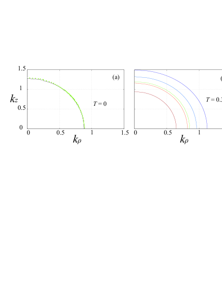
Figure 1: (color online) Contour of the momentum distribution function $n(\mathbf{k})$ for $C_{dd}=1$ at temperatures $T=0$ (a) and 0.3 $T_{F}$ (b). In (a), we draw the Fermi surface. The solid line is the Fermi surface obtained from the self-consistent calculation of this work, the dotted line is the one obtained from the variational approach developed in Refs. taka ; sogo . In (b), the lines from outside to inside correspond to $n(\mathbf{k})=0.1$, 0.3, 0.5, 0.7 and 0.9, respectively.

Results. — Now we present some results. First, let us consider a normal dipolar gas by taking $\Delta(\mathbf{k})=0$. Note that $\Delta=0$ is always a solution to the gap equation (14). Fig. 1 ilustrates the momentum distribution function $n(\mathbf{k})$ as a function of $k_{z}$ and $k_{\rho}=\sqrt{k_{x}^{2}+k_{y}^{2}}$, for two different temperatures. Here the momentum is in units of the Fermi wave number of the non-interacting system $k_{F}=(6\pi^{2}n)^{1/3}$. The dipolar interaction strength is fixed at $C_{dd}=1$ where $C_{dd}=md^{2}n^{1/3}/\hbar^{2}$ is the dimensionless dipolar strength sogo . $C_{dd}=1$ corresponds to the RbK molecule created at the JILA experiment at a modest density of about $4\times 10^{-12}$cm^-3. At $T=0$, $n(\mathbf{k})=v_{\mathbf{k}}^{2}=\Theta(-\epsilon(\mathbf{k}))$, where $\Theta(.)$ is the step function. We draw in Fig. 1(a) the contour of the Fermi surface. In Refs. taka ; sogo , we developed a variational approach and assume that the Fermi surface of the dipolar gas has an ellipsoidal shape:

$$n(\mathbf{k})=\Theta\left(1-\alpha^{2}k_{z}^{2}-k_{\rho}^{2}/\alpha\right)\,.$$

where $\alpha$ is the variational parameter characterizing the deformation of the Fermi surface. At $C_{dd}=1$, we obtain $\alpha=0.7769$. In Fig. 1(a), the dotted line represents the contour of the Fermi surface from this variational calculation. As one can see, the variational result matches with the full self-consistent calculation very well. At larger $C_{dd}$, small difference can be see between the two results. In general, the variational results exhibit slightly stronger deformation. The same conclusion has been reached by Ronen and Bohn ronen . Fig. 1(b) shows the momentum distribution at $T=0.3$ $T_{F}$, respectively, where $T_{F}=E_{F}/k_{B}$ is the Fermi temperature of the non-interacting system. At finite temperature, Fermi surface gets smeared out. However, the anisotropy of the momentum distribution is still quite clear.

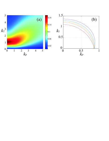
Figure 2: (color online) (a) Gap parameter $\Delta(\mathbf{k})$ (in units of $E_{F}$) at $T=0$ for $C_{dd}=1$. (b) The corresponding contour plot of the momentum distribution function $n(\mathbf{k})$. The lines from outside to inside correspond to $n(\mathbf{k})=0.1$, 0.3, 0.5, 0.7 and 0.9, respectively.

Let us now turn to the discussion of the superfluid state. For simplicity, we take the first-order Born approximation by replacing the vertex function $\Gamma(\mathbf{k}-\mathbf{k}^{\prime})$ in the gap equation (14) by the bare dipolar interaction $U(\mathbf{k}-\mathbf{k}^{\prime})$. This should be a good approximation as long as the dipolar interaction strength is not too strong baranov . In Fig. 2(a), we plot the zero-temperature gap parameter $\Delta(\mathbf{k})$ for $C_{dd}=1$. $\Delta(\mathbf{k})$ is an odd function of $\mathbf{k}$ and vanishes for $k_{z}=0$. As a consequence, the Fermi surface smears out except at $k_{z}=0$, as can be seen from the momentum distribution shown in Fig. 2(b). The peak value of $\Delta$ reaches nearly 0.2$E_{F}$ for this rather modest dipolar interaction strength, and occurs near $k_{z}=k_{F}$ and $k_{\rho}=0$. To investigate the angular distribution of $\Delta$, we note that:

$$\Delta(\mathbf{k})=\Delta(k,\cos\theta_{\mathbf{k}})=\sum_{\mathrm{odd}\,l}\Delta_{l}(k)Y_{l0}(\cos\theta_{\mathbf{k}})\,,$$

where $k=|\mathbf{k}|$ and due to the cylindrical symmetry of the system, only odd $l$ and $m=0$ components are present. In Fig. 3, we plot $\Delta_{l}(k)$ for $C_{dd}=1$. For small values of $k$ ($k\lesssim k_{F}$), $\Delta$ is dominated by the $l=1$ ($p$-wave) component. For larger $k$, contribution from higher partial waves may become important.

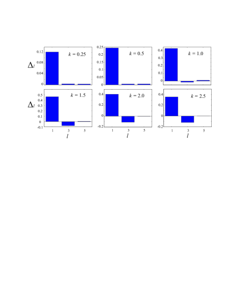
Figure 3: $\Delta_{l}(k)$ for $C_{dd}=1$ at zero temperature.

Next, we illustrate the finite-temperature effects in Fig. 4. The dashed line in Fig. 4(a) represents the chemical potential of the superfluid state as a function of temperature. It increases with temperature. In comparison, the chemical potential of the normal state (the solid line in Fig. 4(a)) is a monotonically decreasing function of temperature. Fig. 4(b) shows how $T_{c}$ varies with $C_{dd}$. The solid line is a fit according to

$$T_{c}/T_{F}=0.8363\,\exp(-2.194/C_{dd})\,.$$ (15)

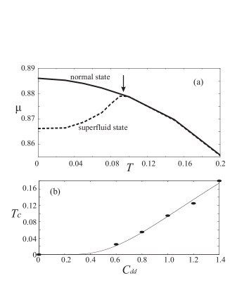
Figure 4: (a) Chemical potential $\mu$ as a function of temperature for superfluid state (dashed line) and normal state (solid line). Energy and temperature are in units of $E_{F}$ and $T_{F}$, respectively. Here $C_{dd}=1$. The arrow indicates the location of $T_{c}$. Superfluid state exists for $0<T<T_{c}$. (b) $T_{c}$ as a function of $C_{dd}$. Here the dots are numerical data and the smooth curve is a fit according to Eq. (15).

Some remarks are in order. First, from our calculation, we find that $T_{c}\approx 0.1T_{F}$ at $C_{dd}=1$. If we were dealing with a two-component Fermi gas with contact interaction, such a critical temperature would correspond to a system inside the unitary regime. As we have mentioned, $C_{dd}=1$ is a quite modest value for polar molecules. Therefore, typical polar molecules can easily reach the “strongly interacting” regime. Second, it is instructive to compare Eq. (15) to the critical temperature found by Baranov et al. baranov which in our notation takes the form:

$$T_{c}/T_{F} \approx 1.44\,\exp\left[-\frac{\pi^{3}}{4(6\pi^{2})^{1/3}C_{dd}}\right]$$

$$= 1.44\,\exp(-1.9887/C_{dd})\,.$$

One can notice that the coefficients in the exponent agree quite well. Less agreement is found in the prefactor. This is, however, understandable as there are several differences in our treatment. For example, Baranov et al. have included beyond-mean-field fluctuation and the contribution from the second-order Born approximation note , while neglected the Fock term in their calculation.

Finally, to reveal the interplay between pairing and Fermi surface deformation, we artifically turn off the Fock term in our calculation. We find that the presence of the Fock exchange interaction increases both the critical temperature and the magnitude of the order parameter by $20\sim 25\%$. This enhancement can be understood in the following way. The presence of the Fock term causes an ellipsoidal deformation of the Fermi surface in such a way that it stretches the momentum distribution along the $z$-axis. As a result, the density of states near the Fermi surface is increased along $z$ and reduced along the transverse directions. On the other hand, the dipolar-induced pairing is dominated by the $p$-wave symmetry, i.e., strongest in the $z$ direction. Therefore, the Fock interaction-induced Fermi surface deformation tends to enhance superfluid pairing.

Conclusion. — We have presented a fully self-consistent Hartree-Fock-Bogoliubov theory to study a system of spinless fermions with long-range interaction. We applied this theory to uniform polar Fermi molecules, calculated the superfluid order paramter and the critical temperature $T_{c}$. Our work shows that: a typical Fermi gas of polar molecules can easily reach the “strongly interacting” regime with $T_{c}$ being a significant fraction of Fermi temperature $T_{F}$, and the Fock interaction has the effect of enhancing superfluid pairing. In the future, it will be of great interest to investigate the collective excitations of the superfluid dipolar Fermi gases, and the effects of quantum fluctuations and the possibility of novel quantum phases that may arise at large dipolar interaction strength and/or in the presence of opitical lattice potential lattice .

This work is supported by the NSF, the Welch Foundation (Grant No. C-1669) and the W.M. Keck Foundation. HP acknowledges the hospitality of Aspen Center for Physics where part of the work is completed.

References

• (1) S. Ospelkaus et al., Nature Phys. 4, 622 (2008); K. K. Ni et al., Science 322, 231 (2008).
• (2) D. DeMille, Phys. Rev. Lett. 88, 067901 (2002).
• (3) A. Micheli et al., Nature Phys. 2, 341 (2006)
• (4) M. A. Baranov et al., Phys. Scr. T102, 74 (2002); M. A. Baranov, Phys. Rep. 464, 71 (2008).
• (5) M. A. Baranov, et al., Phys. Rev. Lett. 94, 070404 (2005); K. Osterloh, et al., ibid. 99, 160403 (2007); H. P. Buchler, et al., ibid. 98, 060404 (2007); G. Pupillo, et al., ibid. 100, 050402 (2008).
• (6) C. -K. Chan et al., arXiv:0906.4403; B. M. Fregoso, K. Sun, E. Fradkin, and B. L. Lev, arXiv.org:0902.0739.
• (7) M. A. Baranov et al., Phys. Rev. A 66, 013606 (2002); M. A. Baranov et al., Phys. Rev. Lett. 92, 250403 (2004).
• (8) G. M. Bruun and E. Taylor, Phys. Rev. Lett. 101, 245301 (2008).
• (9) T. Miyakawa, T. Sogo, and H. Pu, Phys. Rev. A 77, 061603(R) (2008).
• (10) T. Sogo et al., New J. Phys. 11, 055017 (2009).
• (11) S. Ronen et al., arXiv:0906.3753.
• (12) Quantum fluctuations tend to decrease $T_{c}$, while the second-order Born approximation tends to increase $T_{c}$ baranov . Hence these two effects tend to partially cancel each other.
• (13) J. Quintanilla, S. T. Carr and J. J. Betouras, Phys. Rev. A 79, 031601(R) (2009).