Nanoscale Magnetic Heat Pumps and Engines

Abstract

We present the linear response matrix for a sliding domain wall in a rotatable magnetic nanowire, which is driven out of equilibrium by temperature and voltage bias, mechanical torque, and magnetic field. An expression for heat-current induced domain wall motion is derived. Application of Onsager’s reciprocity relation leads to a unified description of the Barnett and Einstein-de Haas effects as well as spin-dependent thermoelectric properties. We envisage various heat pumps and engines, such as coolers driven by magnetic fields or mechanical rotation as well as nanoscale motors that convert temperature gradients into useful work. All parameters (with the exception of mechanical friction) can be computed microscopically by the scattering theory of transport.

I Introduction

Onsager’s reciprocal relationsOnsager reveal that seemingly unrelated phenomena can be expressions of identical microscopic correlations between thermodynamic variables of a given system.Groot The archetypal example is the Onsager-Kelvin identity of thermopower and Peltier cooling.

Research into the interaction between electric currents and the ferromagnetic order parameter of the last years has paid off handsomely. On one hand, the predicted charge current-induced spin transfer torqueBerger ; Slonczewski in metallic ferromagnetic structures such as spin valves and domain wallsTatara ; Klaui ; Ralph in ferromagnetic wires has been understood in some detail and applied to random access magnetic memories,Hitachi logics,Matsunaga and shift registers.Parkin On the other hand, it has been established that a moving magnetization pumps a spin currentTserkovnyak02 that can be converted into charge currents and voltages in ferromagnet$|$normal metal bilayers,Wang ferromagnetic textures,Barnes multilayers,Xiao or by the spin Hall effect.Saitoh Spin-pumping induced voltages have been observed in metallic magnetic heterostructures,Saitoh ; Costache tunnel junctionsMoriyama and magnetic wires with a moving domain wall.Yang A modern illustration of the power of Onsager’s relations is the demonstration that spin-transfer torques and charge currents induced by magnetization dynamics are two sides of the same medal.Saslow ; Duine ; Mecklenburg

Domain walls also react to thermal gradients, as first observed and discussed by Jen and Berger.Berger85 ; Jen1 ; Jen2 Domain wall displacement by laser heating is a possible technology for high-density magnetic recording.Miyakoshi Hatami et al.Hatami and SaslowSaslow proposed a thermoelectric spin-transfer torque as mechanism for magnetization switching in spin valves and domain wall motion in magnetic wires. More recently, Kovalev et al.Kovalev09 addressed this issue for general one-dimensional spin textures in ferromagnetic wires. Yuan et al. found large non-adiabatic corrections to the thermal torques on narrow domain walls.Yuan09

The scattering theory of electron transport can be employed to describe dissipative processes in magnetic systems such as the Gilbert damping of magnetizations dynamics,Brataas08 ; Starikov leading to a microscopic formalism for the Onsager coefficients that govern the interaction between charge currents and magnetization dynamics.Hals ; Hals2

Nearly a century ago it was discovered that in macroscopic bodies the magnetization of a ferromagnet couples to the mechanical degree of freedom: Barnett demonstrated that a mechanical rotation of a demagnetized ferromagnet creates a net magnetization along the rotation axis,Barnett whereas Einstein and de Haas showed that reversing the magnetic moment of a ferromagnetic cylinder induces a mechanical torque.Einstein Both effects are governed by the same gyromagnetic tensor.LLP The microscopic theory of mechanical and magnetic angular momentum coupling in nanostructures has recently been picked up again.Fulde ; Kovalev03 ; Kovalev05 ; Kovalev07 Moreover, Wallis et al.Wallis succeeded in measuring an Einstein-de Haas effect by agitating a magnetic cantilever. Zolfagharkhani et al.Zolfagharkhani detected the mechanical torque induced by the decay of a current-induced magnetization, which can be interpreted as a variation of the Einstein-de Haas effect.Kovalev08 The conditions to observe the Barnett effect in nanostructures have been estimated by Bretzel et al.Bretzel

In this paper we show that effects of magnetic, electric, thermal, and mechanical forces can be unified in a linear response matrix relating the conjugated thermodynamic variables for charge, energy, magnetization, and mechanical rotation. In order to keep mathematics simple, we focus on a thin wire of an easy-plane metallic ferromagnet as studied by Hals et al.Hals for current-induced magnetization dynamics. The wire is connects two heat and particle baths and is allowed to rotate (Figure 1). We may profit from Onsager’s relations according to which we have to fill in only one half of the nondiagonal elements of the response matrix. This implies, for example, that in the linear regime Barnett and Einstein-de Haas effects are equivalent. We identify the heat-current driven domain wall motion and conclude that domain wall motion is associated with the pumping of heat (or a “thermal motive force”). The mechanical torque generated by a temperature difference opens the vista of magnetic nanoscale heat engines.

In this paper we first recapitulate the basic thermodynamics following de GrootGroot for a conventional thermoelectric element in Section IIa. In Section IIb we show that the Onsager principles can be applied to the coupling between magnetic and mechanical dynamics for a model system of a magnetic wire containing a domain wall. In Section III the Onsager matrix is derived for a coupled thermoelectric and magnetomechanical system. In Section IV we specify how the Onsager matrix elements can be computed microscopically. Section V is devoted to a discussion of the magnitude of the couplings for a model system consisting of a nanowire of a ferromagnetic metal wire encapsulated in mult0-wall carbon nanotubes. Section VI summarizes the conclusions.

II Non-equilibrium thermodynamics

According to the second law of thermodynamics the entropy $\mathcal{S}$ is maximal for the equilibrium state such that

$$\Delta\mathcal{S}=-\frac{1}{2}\sum_{i=1}^{n}\sum_{k=1}^{n}g_{ik}a_{i}a_{k}\leq 0$$ (1)

for small deviations of the $n$ state variables $a_{i}=A_{i}-\bar{A}_{i}$ from their equilibrium values $\bar{A}_{i}$. The matrix of coefficients $\hat{g}$ is positive definite and symmetric. If we parameterize a small deviation of the system from thermodynamic equilibrium by the forces (affinities) $X_{i}$ defined by (where $T$ is the equilibrium temperature):

$$X_{i}\equiv T\frac{\partial\mathcal{S}}{\partial a_{i}}=-T\sum_{k=1}^{n}g_{ik}a_{k}\,,$$ (2)

then, in linear response, the variables $A_{i}$ will relax to their equilibrium values $\bar{A}_{i}$ according to

$$J_{i}\equiv\dot{a}_{i}=\sum_{k=1}^{n}L_{ik}X_{k},$$ (3)

defining the response matrix $\hat{L}$. Its elements can be introduced phenomenologically or computed from microscopic principles by the Kubo-Greenwood formalism or scattering theory. The system responses $J_{i}$ are called fluxes, currents, rates, velocities etc. Eq. (3) remains valid in the presence of external forces slowly varying in time that may render the $\bar{A}_{i}$ time dependent. The entropy generation rate reads

$$\dot{\mathcal{S}}=-\sum_{i}\dot{a}_{i}\sum_{k}g_{ik}a_{k}=\frac{1}{T}\sum_{i}J_{i}X_{i}.$$ (4)

Onsager discovered that, due to microscopic time-reversal symmetry, the linear response coefficients obey the reciprocity relations

$$L_{ik}\left(\mathbf{H}_{\mathrm{ext}},\mathbf{m}\right)=\epsilon_{i}\epsilon_{k}L_{ki}\left(-\mathbf{H}_{\mathrm{ext}},-\mathbf{m}\right).$$ (5)

where $\epsilon_{i}=1$ if the state variable $a_{i}$ is even under time reversal and $\epsilon_{i}=-1$ otherwise. Time-reversal (anti)symmetry in the presence of external magnetic fields $\mathbf{H}_{\mathrm{ext}}$ and equilibrium magnetic ordering indicated by a vector field with unit length $\mathbf{m}(\mathbf{r})$ (parametrizing the position-dependent direction of the magnetization) has been made explicit. The inverse of the response matrix $\hat{L}:$

$$X_{i}=\sum_{k=1}^{n}L_{ik}^{-1}J_{k},$$ (6)

has the same Onsager symmetry

$$L_{ik}^{-1}\left(\mathbf{H}_{\mathrm{ext}},\mathbf{m}\right)=\epsilon_{i}\epsilon_{k}L_{ki}^{-1}\left(-\mathbf{H}_{\mathrm{ext}},-\mathbf{m}\right).$$ (7)

II.1 Thermoelectric element

Consider as an example an ordinary thermoelectric element (such as a wire) connecting two reservoirs which are in respective thermal equilibria but at different temperatures $T_{1}/T_{2}$ and voltages $V_{1}\$/$V_{2}$. Let us define $\Delta T=T_{2}-T_{1}\ll T$ and $\Delta V=V_{2}-V_{1}$. If the wire has no independent degrees of freedom, we can describe a general (slightly out-of-equilibrium) state of this closed system by (half of) the energy and charge differences between the two reservoirs, $U=(U_{2}-U_{1})/2$ and $q=(q_{2}-q_{1})/2$, respectively. Disregarding the wire’s heat capacity and electrostatic capacitance relative to those of the large reservoirs, $U$ and $q$ correspond to the energy and charge that have been transferred from reservoir 1 (left) to reservoir 2 (right) with respect to some reference state. $J_{c}=\dot{q}$ and $J_{Q}=\dot{U}$ are, respectively, charge and energy currents associated with $U$ and $q$ that are driven by $\Delta T$ and $\Delta V$. We next employ the thermodynamic identity

$$T_{j}\dot{\mathcal{S}}_{j}=\dot{U}_{j}-V_{j}\dot{q}_{j}\,,$$ (8)

which holds for each reservoir separately. To leading order in the perturbations, the total entropy change $\dot{\mathcal{S}}=\dot{\mathcal{S}}_{1}+\dot{\mathcal{S}}_{2}$ introduced by moving a small amount of energy and charge between the reservoirs is thus

$$T\mathcal{\dot{S}}=-\frac{\Delta T}{T}\dot{U}-\Delta V\dot{q}$$ (9)

By comparison with Eq. (4), we identify the conjugate fluxes and forces:

$$J_{Q}=\dot{U}\,,\;X_{Q}=-\frac{\Delta T}{T}\,;\;J_{c}=\dot{q}\,,\;X_{c}=-\Delta V\,,$$ (10)

such that Eq. (3) becomes

$$\left(\begin{array}[c]{c}J_{c}\\ J_{Q}\end{array}\right)=\left(\begin{array}[c]{cc}L_{11}&L_{12}\\ L_{21}&L_{22}\end{array}\right)\left(\begin{array}[c]{c}-\Delta V\\ -\frac{\Delta T}{T}\end{array}\right).$$ (11)

The Onsager matrix can be rewritten in terms of the electric conductance

$$G=-\left.\frac{J_{c}}{\Delta V}\right|_{\Delta T=0},$$ (12)

heat conductance

$$\kappa=-\left.\frac{J_{Q}}{\Delta T}\right|_{J_{c}=0},$$ (13)

and thermopower or Seebeck coefficient

$$S=\left.-\frac{\Delta V}{\Delta T}\right|_{J_{c}=0},$$ (14)

such that

$$\left(\begin{array}[c]{c}J_{c}\\ J_{Q}\end{array}\right)=\left(\begin{array}[c]{cc}G&GTS\\ GTS&TG\left(\frac{\kappa}{G}+TS^{2}\right)\end{array}\right)\left(\begin{array}[c]{c}-\Delta V\\ -\frac{\Delta T}{T}\end{array}\right).$$ (15)

Traditionally, the role of currents and voltages in the thermoelectric response are exchanged. In terms of the resistance $R=1/G:$

$$\left(\begin{array}[c]{c}-\Delta V\\ J_{Q}\end{array}\right)=\left(\begin{array}[c]{cc}R&-TS\\ TS&T\kappa\end{array}\right)\left(\begin{array}[c]{c}J_{c}\\ -\frac{\Delta T}{T}\end{array}\right).$$ (16)

Hereby, we recovered the Onsager-Kelvin relation between thermopower and Peltier coefficient:

$$\Pi\equiv\left.\frac{J_{Q}}{J_{c}}\right|_{\Delta T=0}=TS\,.$$ (17)

The Sommerfeld approximation leads to the Wiedemann-Franz law $\kappa=G\mathcal{L}T\$and Mott’s formula $S=-e\mathcal{L}T\partial_{E}\ln G|_{E_{F}},$ where $\partial_{E}\ln G|_{E_{F}}$ is the logarithmic energy derivative of the conductance at the Fermi energy $E_{F}$, $\mathcal{L}=(k_{B}/e)^{2}\pi^{2}/3$ is the Lorenz number and $-e$ the electron charge. The dimensionless expression $S^{2}/\mathcal{L}$ vanishes quadratically at low temperatures, is small for most metals at room temperature,Hatami and may usually be disregarded. Eq. (15) then becomes

$$\left(\begin{array}[c]{c}J_{c}\\ J_{Q}\end{array}\right)=G\left(\begin{array}[c]{cc}1&TS\\ TS&\mathcal{L}T^{2}\end{array}\right)\left(\begin{array}[c]{c}-\Delta V\\ -\frac{\Delta T}{T}\end{array}\right)\,,$$ (18)

II.2 Magnetomechanical element

We consider now a quasi-one-dimensional magnetic nanowire with easy-plane anisotropy that contains a transverse domain wall, which is the standard model system for the study of magnetic domain wall motion. We chose here the tail-to-tail (rather than head-to-head) topology shown in Figure 1. The wire is mounted in a low-friction bearing such that it can freely rotate around its ($x$) axis and a mechanical torque $\tau_{\mathrm{ext}}^{\mathrm{mech}}$ can be applied. The system can also be driven by an applied magnetic field $H_{\mathrm{ext}}$, and, via electric and thermal contacts, by a voltage $\left(\Delta V\right)$ and/or temperature $\left(\Delta T\right)$ bias.

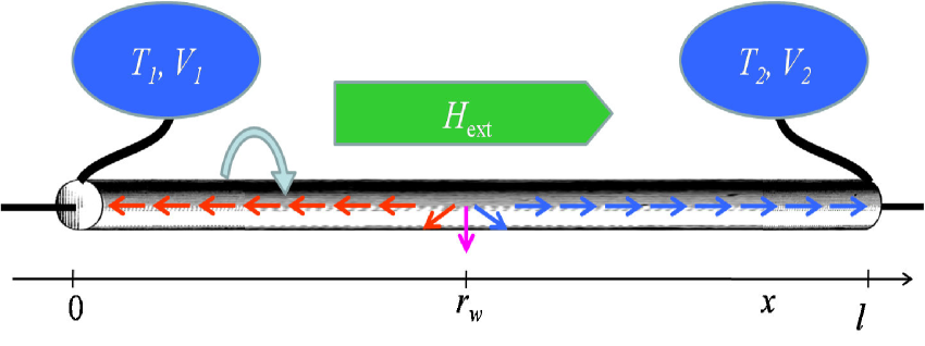
Figure 1: Magnetic nanowire of length $l$ in electrical and thermal contact with reservoirs. A domain wall is centered at position $r_{w}$. The wire is mounted such that it can rotate around the $x$-axis. A magnetic field and mechanical torque can be applied along $x.$

Let us suppose initially that the magnetomechanical properties are decoupled from the electric and heat currents. The equation of motion of the magnetization $M_{s}\mathbf{m}\left(x,t\right)\mathbf{,}$ where $M_{s}$ is the constant saturation magnetization, is governed by the Landau-Lifshitz-Gilbert (LLG) equation, appended by Barnett’s gauge field that represents the aligning torque felt by angular momenta in rotating systems. In the frame of reference that rotates with the wire:Bretzel

$$\dot{\mathbf{m}}=-\gamma\mathbf{m}\times\mathbf{H}_{\mathrm{eff}}+\alpha\mathbf{m}\times\dot{\mathbf{m}}+\mathbf{m}\times\mathbf{x}\dot{\varphi}\,,$$ (19)

where $\gamma$ is the minus the gyromagnetic ratio ($\gamma>0$ for electrons) and $\dot{\varphi}$ the angular velocity of the wire around its axis. The effective field $\mathbf{H}_{\mathrm{eff}}$ is the functional derivative of the free energy $\mathcal{F}$ with respect to the magnetization at rest, which has contributions from the applied, anisotropy, and exchange magnetic fields:

$$\mathbf{H}_{\mathrm{eff}}=-\frac{\delta\mathcal{F}\left[\mathbf{m}\right]}{M_{s}\delta\mathbf{m}\left(\mathbf{r}\right)}=(H_{\mathrm{ext}}+Km_{x})\mathbf{x}-K_{\perp}m_{z}\mathbf{z}+A_{\mathrm{ex}}\nabla^{2}\mathbf{m}\,,$$ (20)

where $\mathbf{m}\equiv(m_{x},m_{y},m_{z})=(\cos\theta,\sin\theta\cos\phi,\sin\theta\sin\phi)$, the anisotropy constants $K>0$, $K_{\perp}>0,$ and the exchange stiffness $A_{\mathrm{ex}}\$have been introduced. In the absence of pinning the Walker ansatzSchryer

$$\ln\tan\frac{\theta(x,t)}{2}=-\frac{x-r_{w}(t)}{\lambda_{w}}\,\,\,\mathrm{and}\,\,\,\phi\left(x,t\right)=\phi(t)\,,$$ (21)

provides a solution in terms of a domain wall with time-dependent position $r_{w}$ and (squared) width $\lambda_{w}^{2}=A_{\mathrm{ex}}/(K+K_{\perp}\sin^{2}\phi).$ The polar angle $\phi$ is the tilt of the magnetization against the easy-plane anisotropy $K_{\perp}$, which vanishes at equilibrium. $\phi$ is a constant for sufficiently small, steady-state driving forces, and therefore not a dynamic variable in the regimes considered henceforth. Substituting Eq. (21) into the Landau-Lifshitz-Gilbert Eq. (19)

$$\dot{r}_{w}=\frac{\lambda_{w}}{\alpha}(\dot{\varphi}-\gamma H_{\mathrm{ext}})\,,\;K_{\perp}\sin 2\phi=-\frac{2(\dot{\varphi}-\gamma H_{\mathrm{ext}})}{\alpha\gamma}\,.$$ (22)

This solution is valid up to a critical (Walker) threshold field at which $|\sin 2\phi_{W}|=1$. To linear order in the driving field, we can approximate the domain wall width $\lambda_{w}$ by its equilibrium value, $\lambda_{w}=\sqrt{A_{\mathrm{ex}}/K}$.

The mechanical rotation of the wire is governed by the damped oscillator equation:

$$I\ddot{\varphi}+\beta^{\mathrm{mech}}\dot{\varphi}=\tau^{\mathrm{mech}},$$ (23)

where $\beta^{\mathrm{mech}}$ is the mechanical damping parameter and $\tau^{\mathrm{mech}}$ the total mechanical torque acting along the $x$-axis. The total angular momentum $\mathfrak{L}_{\mathrm{axis}}$ of the mechanical and magnetic subsystems in a freely rotating wire of cross section $A$

$$\mathfrak{L}_{\mathrm{axis}}=-\frac{AM_{s}}{\gamma}\left(l-2r_{w}\right)+I\dot{\varphi}\,,$$ (24)

is dissipated into the environment at a rate $\mathfrak{\dot{L}}_{\mathrm{axis}}=-\beta^{\mathrm{mech}}\dot{\varphi}$. This leads to an expression for the Einstein-de Haas torque induced by a moving domain wall:

$$\tau_{\mathrm{EdH}}^{\mathrm{mech}}=-\frac{2AM_{s}}{\gamma}\dot{r}_{w}.$$ (25)

We assume in the following that the system is overdamped, i.e., we limit our attention to frequencies smaller than $\beta/I$, such that the acceleration $\ddot{\varphi}$ and moment of inertia $I$ drop out of the problem. The rotation velocity is then directly proportional to the total torque $\tau^{\mathrm{mech}}=\tau_{\mathrm{ext}}^{\mathrm{mech}}+\tau_{\mathrm{EdH}}^{\mathrm{mech}}$:

$$\beta^{\mathrm{mech}}\dot{\varphi}=\tau_{\mathrm{ext}}^{\mathrm{mech}}-\frac{2AM_{s}}{\gamma}\dot{r}_{w}\,.$$ (26)

The mechanical energy $E(\varphi)$ governs the external torque, $\tau_{\mathrm{ext}}^{\mathrm{mech}}\equiv-\partial_{\varphi}E(\varphi)$.

The above results will now be shown to be consistent with Onsager’s reciprocity principle and the second law of thermodynamics. Disregarding thermal effects, it is natural to switch to the free energy $\mathcal{F}$ instead of the entropy $\mathcal{S}$:

$$\mathcal{F}(r_{w},\varphi)=\mathcal{F}_{w}+\mathcal{F}_{\varphi}=(2r_{w}-l)AM_{s}H_{\mathrm{ext}}+E(\varphi)\,,$$ (27)

where $l$ is the total length of the wire and the domain wall position $r_{w}$ is measured with respect to the left end of the wire. We omit the internal energy of the domain wall, which below the Walker threshold may be treated as a rigid particle-like mass-less object specified by its position. The conjugate forces associated with $r_{w}$ and $\varphi$ are immediately found as

$$X_{w}\equiv-\frac{\partial}{\partial r_{w}}\mathcal{F}=-2AM_{s}H_{\mathrm{ext}}\,;\;X_{\varphi}\equiv-\frac{\partial}{\partial\varphi}\mathcal{F}=\tau_{\mathrm{ext}}^{\mathrm{mech}}\,.$$ (28)

After simple algebra using Eqs. (22) and (26), the energy dissipation is found to be positive definite:

$$T\dot{\mathcal{S}}\equiv-\dot{\mathcal{F}}=-2AM_{s}H_{\mathrm{ext}}\dot{r}_{w}+\tau_{\mathrm{ext}}^{\mathrm{mech}}\dot{\varphi}=\frac{2\alpha AM_{s}}{\gamma\lambda_{w}}\dot{r}_{w}^{2}+\beta^{\mathrm{mech}}\dot{\varphi}^{2}\geq 0\,,$$ (29)

Rewriting the equations of motion (22) and (26), the cross terms are seen to obey Onsager’s symmetry:

$$\left(1+\frac{2AM_{s}}{\gamma}\frac{\lambda_{w}}{\alpha\beta^{\mathrm{mech}}}\right)\left(\begin{array}[c]{c}\dot{\varphi}\\ \dot{r}_{w}\end{array}\right)=\left(\begin{array}[c]{cc}\frac{1}{\beta^{\mathrm{mech}}}&-\frac{\lambda_{w}}{\alpha\beta^{\mathrm{mech}}}\\ \frac{\lambda_{w}}{\alpha\beta^{\mathrm{mech}}}&\frac{\lambda_{w}\gamma}{2\alpha AM_{s}}\end{array}\right)\left(\begin{array}[c]{c}X_{\varphi}\\ X_{w}\end{array}\right)\$$ (30)

The antisymmetry of the off-diagonal terms stems from Onsager’s reciprocity, which relates here the response of the tail-to-tail domain wall to that of its time-reversed partner, which is a head-to-head domain wall. Note that the inverse of Eq. (30) is simpler

$$\left(\begin{array}[c]{c}X_{\varphi}\\ X_{w}\end{array}\right)=\left(\begin{array}[c]{cc}\beta^{\mathrm{mech}}&\frac{2AM}{\gamma}\\ -\frac{2AM}{\gamma}&\frac{2AM}{\gamma}\frac{\alpha}{\lambda}\end{array}\right)\left(\begin{array}[c]{c}\dot{\varphi}\\ \dot{r}_{w}\end{array}\right),\$$ (31)

but Eq. (30) should be closer to experimental set-ups in practice. We may rewrite it as

$$\left(\begin{array}[c]{c}\dot{\varphi}\\ \dot{r}_{w}\end{array}\right)=\left(\begin{array}[c]{cc}\frac{1}{\tilde{\beta}^{\mathrm{mech}}}&-\frac{\lambda_{w}}{\tilde{\alpha}\beta^{\mathrm{mech}}}\\ \frac{\lambda_{w}}{\tilde{\alpha}\beta^{\mathrm{mech}}}&\frac{\lambda_{w}\gamma}{2\tilde{\alpha}AM_{s}}\end{array}\right)\left(\begin{array}[c]{c}X_{\varphi}\\ X_{w}\end{array}\right)\,,$$ (32)

where

$$\tilde{\beta}^{\mathrm{mech}} =\beta^{\mathrm{mech}}+\frac{2\lambda_{w}AM_{s}}{\alpha\gamma}\,,$$

$$\tilde{\alpha} =\alpha+\frac{2\lambda_{w}AM_{s}}{\gamma\beta^{\mathrm{mech}}}\,.$$ (33)

The magnetomechanical coupling creates an apparently increased damping of the magnetization dynamics and/or the mechanical motion that is proportional to the number of spins in the domain wall. $\beta^{\mathrm{mech}}$ is the mechanical friction: when it becomes large the mechanical motion is quenched and the excess Gilbert damping is suppressed $\tilde{\alpha}\rightarrow\alpha$. In turn, the direct coupling of the mechanical torque to the rotation, $L_{\varphi\varphi}=1/\tilde{\beta}^{\mathrm{mech}}$, vanishes with vanishing Gilbert damping $\alpha$, i.e., $\tau_{\mathrm{ext}}^{\mathrm{mech}}$ is fully transferred into the magnetic system. For vanishing mechanical damping $\beta^{\mathrm{mech}}$, the domain wall remains immobile under a magnetic field, but the wire rotates with an $\alpha$-independent angular velocity, which exactly compensates the external field in the rotating frame (i.e., $\dot{\varphi}=\gamma H_{\mathrm{ext}}$). These results are valid only in the steady-state, overdamped mechanical regime considered here.

III Magnetomechanothermoelectric systems

We now define the conjugate thermodynamical variables $a_{i}$ that allow us to take advantage of Onsager’s relations as energy transfer $U=(U_{2}-U_{1})/2$, charge transfer $q=(q_{2}-q_{1})/2$, domain wall position $r_{w}$, and lattice-rotation angle $\varphi.$ The corresponding fluxes are given by their time derivatives $J_{Q}=\dot{U},$ $J_{c}=\dot{q},$ $J_{w}=\dot{r}_{w},$ $J_{\varphi}=\dot{\varphi}$. The thermodynamic forces (2) depend in principle on the values of all thermodynamic variables. It is possible to work out a general scheme that includes all possible cross correlations, but it would not be very transparent. Instead, we follow a more pragmatic approach that is based on the low-temperature free energy for the magnetomechanical degrees of freedom, which are coupled to thermoelectric transport between the reservoirs by the spin torques. The linear response matrix then reads $\mathbf{J}=\hat{L}\mathbf{X}$, where

$$\mathbf{J} =\left(\begin{array}[c]{cccc}J_{c},&J_{Q},&\dot{\varphi},&\dot{r}_{w}\end{array}\right)^{T}$$ (35)

$$\mathbf{X} =\left(\begin{array}[c]{cccc}-\Delta V,&-\frac{\Delta T}{T},&\tau_{\mathrm{ext}}^{\mathrm{mech}},&-2AM_{s}H_{\mathrm{ext}}\end{array}\right)^{T}$$ (37)

and

$$\hat{L}=\left(\begin{array}[c]{cccc}L_{cc}&L_{cQ}&L_{c\varphi}&L_{cw}\\ L_{Qc}&L_{QQ}&L_{Q\varphi}&L_{Qw}\\ L_{\varphi c}&L_{\varphi Q}&L_{\varphi\varphi}&L_{\varphi w}\\ L_{wc}&L_{wQ}&L_{w\varphi}&L_{ww}\end{array}\right).$$ (38)

When thermoelectric and magnetomechanical systems are uncoupled, the matrix elements derived in Sec. II may be filled in unmodified. According to the Onsager symmetry, $L_{xw}(\mathbf{m})=L_{wx}(-\mathbf{m})=L_{wx}(\mathbf{m})$ and $L_{x\varphi}(\mathbf{m})=L_{\varphi x}(-\mathbf{m})=-L_{\varphi x}(\mathbf{m})$, for $x=(c,Q)$, assuming that our system obeys a structural mirror symmetry with respect to a plane normal to the wire in Fig. 1. It is useful to introduce also the inverse matrix $\mathbf{X}$ $=\hat{L}^{-1}\mathbf{J}$, recalling that $\hat{L}^{-1}$ and $\hat{L}$ have the same Onsager symmetry.

We can draw a number of conclusions from the Onsager relations already. $L_{wc}$ and $L_{cw}$ represent the Onsager equivalent pair of current-induced transfer torque and charge pumping by the magnetization dynamics, respectively.Saslow ; Duine ; Mecklenburg We know that a temperature gradient can induce a spin-transfer torque,Hatami which is here represented by $L_{wQ}.$ According to Onsager symmetry an opposite and equivalent effect exists, i.e., a heat current induced by magnetization dynamics, which might be applied for cooling or heating purposes. As explained above, the mechanical motion induced by the magnetic field as quantified by $L_{\varphi w}$ (Einstein-de Haas effect) is identical with the Barnett response function $-L_{w\varphi},$ which describes the magnetization dynamics induced by rotation (Barnett effect). Since $L_{\varphi c}=-L_{c\varphi}$ the magnetic wire can be employed as an electromotorKovalev03 and electric generator. A temperature gradient induces a rotation of the wire via $L_{\varphi Q}$, which leads to the prediction of a heat engine that can carry out mechanical work under a temperature difference. The opposite effect, in which mechanical motion of the wire is transformed into a temperature gradient is governed by $L_{Q\varphi}=-L_{\varphi Q}$.

The remaining task is to work out the elements of the $4\times 4$ response matrix. In the adiabatic regime, the magnetic texture varies slowly with respect to the magnetic coherence length $1/\lambda_{c}=|1/\lambda_{F}^{\downarrow}-1/\lambda_{F}^{\uparrow}|,$ where $\lambda_{F}^{\uparrow\left(\downarrow\right)}$ are the spin-dependent Fermi wavelengths and $\uparrow/\downarrow$ denote the majority/minority spin carriers, respectively. The spin torque on, or angular momentum transfer to, the magnetization induced by an applied voltage (superscript $\left(0\right)$ indicates a static magnetization texture and the absence of thermoelectric effects) reads Zhang ; Thiaville ; Mougin ; Tatara ; Tserkovnyak08

$$\left(\mbox{\boldmath$\tau$}_{c}^{\mathrm{mag}}\right)^{\left(0\right)}=-\frac{\hbar}{e}\frac{\gamma}{2AM_{s}}PG\Delta V\left(1-\beta_{c}^{\mathrm{mag}}\mathbf{m}\times\right)\frac{\partial}{\partial x}\mathbf{m}\,.$$ (39)

in terms of the spin polarization $P=\left(G_{\uparrow}-G_{\downarrow}\right)/G$ of the electric conductance $G=G_{\uparrow}+G_{\downarrow}$ of the single-domain ferromagnet. The prefactor (torque in the plane of the domain wall magnetization) can be easily identified as the angular momentum rate of change of the spin-polarized carriers that corresponds to an adiabatic spin reversal. The out-of-plane torque components is caused by the mistracking of the spin in the magnetization texture that is parameterized by $\beta_{c}^{\mathrm{mag}}$. The torque by the thermoelectric spin current induced by a temperature bias (superscript $\left(0\right)$ again denoting a static texture and the condition $S^{2}/\mathcal{L}\ll 1)$ reads analogously:

$$\left(\mbox{\boldmath$\tau$}_{Q}^{\mathrm{mag}}\right)^{\left(0\right)}=-\frac{\hbar}{e}\frac{\gamma}{2AM_{s}}P^{\prime}SG\Delta T\left(1-\beta_{Q}^{\mathrm{mag}}\mathbf{m}\times\right)\frac{\partial}{\partial x}\mathbf{m}\,.$$ (40)

where $P^{\prime}=\partial_{E}\left(PG\right)/\partial_{E}G$ is the polarization of the energy derivative of the conductance.Note The parameter $\beta_{Q}^{\mathrm{mag}}$ parameterizing the out-of-plane torque component differs from $\beta_{c}^{\mathrm{mag}}$ since the non-equilibrium energy distribution defining the spin current through the texture has a node at the Fermi energy rather than a maximum. The Seebeck coefficient for the homogeneous ferromagnet $S=\left(S_{\uparrow}G_{\uparrow}+S_{\downarrow}G_{\downarrow}\right)/G.$

In the coupled system, torques are induced by the magnetization and mechanical motion as well, which can be fully included into the equations of motion by adapting the charge and heat currents, rather than voltage and temperature as system variables (forces). The transformation can be carried out very generally, but leads to different parameters for the out-of-plane torques.Kovalev09 By inverting the thermoelectric matrix in the Sommerfeld approximation and assuming $S^{2}/\mathcal{L}\ll 1,$ the $\beta$ parameters remain unmodified for the current biased torques, however. The torque induced by a heat current $J_{Q}$ then reads

$$\mbox{\boldmath$\tau$}_{Q}^{\mathrm{mag}}=\frac{\hbar}{e}\frac{\gamma}{2AM_{s}}\frac{P^{\prime}S}{\mathcal{L}T}J_{Q}\left(1-\beta_{Q}^{\mathrm{mag}}\mathbf{m}\times\right)\frac{\partial}{\partial x}\mathbf{m}\,,$$ (41)

whereas the charge current torque becomes

$$\mbox{\boldmath$\tau$}_{c}^{\mathrm{mag}}=\frac{\hbar}{e}\frac{\gamma}{2AM_{s}}P\left(J_{c}-\frac{S}{\mathcal{L}T}J_{Q}\right)\left(1-\beta_{c}^{\mathrm{mag}}\mathbf{m}\times\right)\frac{\partial}{\partial x}\mathbf{m}\,.$$ (42)

Note that the conventional thermoelectric charge current has been subtracted here from the total charge current. Adding the spin torques (41) and (42) to the right-hand side of the LLG Eq. (19), we can employ the Walker ansatz again to solve for the current driven domain-wall velocity:

$$\dot{r}_{w}|_{J_{c},J_{Q}}=-\frac{\hbar G}{e}\frac{\gamma}{2AM_{s}}\frac{1}{\alpha}\left(P\beta_{c}^{\mathrm{mag}}\left(J_{c}-\frac{S}{\mathcal{L}T}J_{Q}\right)+\frac{P^{\prime}S}{\mathcal{L}T}\beta_{Q}^{\mathrm{mag}}J_{Q}\right).$$ (43)

A negative charge, thus positive particle, current and $P\beta_{c}^{\mathrm{mag}}>0$ pushes the domain wall to the right. For an electron-like thermopower ($S<0$) and $P^{\prime}\beta_{Q}^{\mathrm{mag}}>0$, a positive heat current has the same effect.

In order to relate $\dot{\varphi}$ to the mechanical torque and identify the unknown response coefficients in Eq. (38), we need to generalize the conservation of angular momentum, Eq. (26), to account for the spin currents injected into and drained from the leads by

$$\beta^{\mathrm{mech}}\dot{\varphi}=\tau_{\mathrm{ext}}^{\mathrm{mech}}-\frac{2AM_{s}}{\gamma}\dot{r}_{w}+\tau_{\mathrm{inj}}^{\mathrm{mech}}\,,$$ (44)

with, for the present choice of magnetization texture,

$$\tau_{\mathrm{inj}}^{\mathrm{mech}}=-\frac{\hbar}{e}(\gamma_{c}P\left(J_{c}-\frac{S}{\mathcal{L}T}J_{Q}\right)+\gamma_{Q}\frac{P^{\prime}S}{\mathcal{L}T}J_{Q}).$$ (45)

The effect is maximized ($\gamma_{c}=\gamma_{Q}=1$) when the angular momentum is drained completely from the wire into the reservoirs. In the opposite limit, the spin currents are dissipated completely in the wire (rather than in the reservoir), as in sufficiently long normal metal terminals to the ferromagnet (N$|$F$|$N) that are part of the mounted wire, such that $\tau_{\mathrm{inj}}^{\mathrm{mech}}=0$. The domain wall equation of motion, including the Barnett torques induced by rotation, reads

$$\dot{r}_{w}=-\frac{\lambda_{w}\gamma}{\alpha}\left(H_{\mathrm{ext}}-\frac{\dot{\varphi}}{\gamma}\right)+\dot{r}_{w}|_{J_{c},J_{Q}}\,.$$ (46)

From Eqs. (43,44,45,46) we can specify all coefficients of the inverse response matrix

$$\hat{L}^{-1}=\left(\begin{array}[c]{cccc}\frac{1}{\kappa}\left(TS^{2}+\frac{\kappa}{G}\right)&-\frac{S}{\kappa}&-\frac{\hbar}{e}P\gamma_{c}&\frac{\hbar}{\lambda_{w}e}P\beta_{c}^{\mathrm{mag}}\\ -\frac{S}{\kappa}&\frac{1}{T\kappa}&-\frac{\hbar}{e}\left(P^{\prime}\gamma_{Q}-P\gamma_{c}\right)\frac{S}{\mathcal{L}T}&\frac{\hbar}{e}\frac{S}{\lambda_{w}\mathcal{L}T}\left(P^{\prime}\beta_{Q}^{\mathrm{mag}}-P\beta_{c}^{\mathrm{mag}}\right)\\ \frac{\hbar}{e}P\gamma_{c}&\frac{\hbar}{e}\frac{S}{\mathcal{L}T}\left(P^{\prime}\gamma_{Q}-P\gamma_{c}\right)&\beta^{\mathrm{mech}}&\frac{2AM_{s}}{\gamma}\\ \frac{\hbar}{\lambda_{w}e}P\beta_{c}^{\mathrm{mag}}&\frac{\hbar}{e}\frac{S}{\lambda_{w}\mathcal{L}T}\left(P^{\prime}\beta_{Q}^{\mathrm{mag}}-P\beta_{c}^{\mathrm{mag}}\right)&-\frac{2AM_{s}}{\gamma}&\frac{2AM_{s}\alpha}{\gamma\lambda_{w}}\end{array}\right)$$ (47)

This representation appears to be less convenient for comparison with practical experiment. In a purely electric circuit it is possible to freely change from a current-biased to a voltage bias set-up. This appears less convenient for the other sets of conjugate variables. It is therefore necessary to adopt the results to the experimental problem at hand. For a set-up in which the driving forces are the $X_{i}$ considered here, it is appropriate to invert the above matrix in order to obtain experimentally more relevant response functions. We have seen in the previous section that for the purely magnetomechanical system the inversion is equivalent to a renormalization of the damping constants. The inversion of the $4\times 4$ matrix leads to lengthy expressions that cannot be interpreted that easily. The simplest approach is second order perturbation theory to estimate the importance of the self-consistent couplings. The diagonal elements of the response matrix then read

$$L_{ii}\approx\frac{1}{\left(L^{-1}\right)_{ii}}\left(1+\sum_{j\neq i}\frac{\left(L^{-1}\right)_{ij}\left(L^{-1}\right)_{ji}}{\left(L^{-1}\right)_{ii}\left(L^{-1}\right)_{jj}}\right),$$ (48)

while the non-diagonal elements become

$$L_{ij}\approx\frac{\left(L^{-1}\right)_{ji}}{\left(L^{-1}\right)_{ii}\left(L^{-1}\right)_{jj}}$$ (49)

In Eq. (47) the $2\times 2$ thermoelectric matrix and the mechanical diagonal elements scale with the system length and inversely with the wire cross section $l/A$, whereas all others are independent of the system size. The non-diagonal block matrices may therefore be treated by perturbation theory in the long and/or narrow wire limit. By defining the block-diagonal matrix

$$\hat{L}_{0}^{-1}=\left(\begin{array}[c]{cccc}\frac{1}{\kappa}\left(TS^{2}+\frac{\kappa}{G}\right)&-\frac{S}{\kappa}&0&0\\ -\frac{S}{\kappa}&\frac{1}{T\kappa}&0&0\\ 0&0&\beta^{\mathrm{mech}}&\frac{2AM_{s}}{\gamma}\\ 0&0&-\frac{2AM_{s}}{\gamma}&\frac{2AM_{s}}{\gamma}\frac{\alpha}{\lambda}\end{array}\right).$$ (50)

and treating $\delta\hat{L}^{-1}=$ $\hat{L}^{-1}-\hat{L}_{0}^{-1}\$ as a perturbation, we find to lowest order in $\delta\hat{L}^{-1}$

$$\hat{L}\approx\hat{L}_{0}-\hat{L}_{0}\delta\hat{L}^{-1}\hat{L}_{0}.$$ (51)

Using the Sommerfeld approximation and letting $S^{2}/\mathcal{L}\rightarrow 0$, we obtain the elements of the lower non-diagonal block as:

$$L_{wc}=-\frac{\hbar}{e}\frac{\gamma}{2AM_{s}}\frac{G}{\tilde{\alpha}}P\left(\beta_{c}^{\mathrm{mag}}+\frac{2AM_{s}}{\gamma}\frac{\lambda_{w}}{\beta^{\mathrm{mech}}}\gamma_{c}\right),$$ (52)

$$L_{wQ}=-\frac{\hbar}{e}\frac{\gamma}{2AM_{s}}\frac{GST}{\tilde{\alpha}}P^{\prime}\left(\beta_{Q}^{\mathrm{mag}}+\frac{2AM_{s}}{\gamma}\frac{\lambda_{w}}{\beta^{\mathrm{mech}}}\gamma_{Q}\right),$$ (53)

$$L_{\varphi c}=-\frac{\hbar}{e}\frac{G}{\tilde{\beta}^{\mathrm{mech}}}P\left(\gamma_{c}-\frac{\beta_{c}^{\mathrm{mag}}}{\alpha}\right),$$ (54)

$$L_{\varphi Q}=-\frac{\hbar}{e}\frac{GST}{\tilde{\beta}^{\mathrm{mech}}}P^{\prime}\left(\gamma_{Q}-\frac{\beta_{Q}^{\mathrm{mag}}}{\alpha}\right).$$ (55)

The perturbation expansion holds well for the example treated below. If it turns out inaccurate, the full matrix should be diagonalized, of course.

In strongly spin-orbit coupled systems the transport polarizations $P$,$P^{\prime}$ are not well defined.Kovalev09 However, the dynamics is governed only by the combinations $P\beta_{c}^{\mathrm{mag}},P\gamma_{c},P^{\prime}\beta_{Q}^{\mathrm{mag}},P^{\prime}\gamma_{Q}$, which can still be determined.Hals3 An important handle to experimental access to the different parameters is a comparison of heat-current driven domain wall motion for both closed and open electric circuits. In the limit $1/\beta^{\mathrm{mech}}=H_{\mathrm{ext}}=0$, the former case leads to

$$\dot{r}_{w}|_{\Delta V=0}=-\frac{\gamma}{2AM_{s}}\frac{\hbar GST}{e}\frac{P^{\prime}\beta_{Q}^{\mathrm{mag}}}{\alpha}\left(-\frac{\Delta T}{T}\right)$$ (56)

whereas

$$\dot{r}_{w}|_{J_{c}=0}=-\frac{\gamma}{2AM_{s}}\frac{\hbar GST}{e}\frac{P^{\prime}\beta_{Q}^{\mathrm{mag}}-P\beta_{c}^{\mathrm{mag}}}{\alpha}\left(-\frac{\Delta T}{T}\right)$$ (57)

An interesting simplified system consists of a completely pinned magnetic domain wall. In this regime, the magnetic degrees of freedom drop out of the problem.Note2 In the adiabatic limit, the spin current then transfers all angular momentum directly to the lattice. Since the magnetization does not move, there is no magnetic dissipation. The response functions in that limit (indicated by a prime) are obtained in the limit $\alpha\rightarrow\infty$ and are significantly simplified

$$L_{\varphi c}^{\prime}=-\frac{\hbar}{e}\frac{G}{\beta^{\mathrm{mech}}}P\gamma_{c},$$ (58)

$$L_{\varphi Q}^{\prime}=-\frac{\hbar}{e}\frac{GST}{\beta^{\mathrm{mech}}}P^{\prime}\gamma_{Q}.$$ (59)

The Onsager equivalent to the current-induced rotation is the rotation-induced charge and heat pumping by the otherwise fixed magnetization texture in the domain wall. It can be explained in terms of the magnetization texture that carries out a rotation rather than a translation, which in the rotating frame results in an effective (Barnett-like) field $\dot{\varphi}/\gamma$ between the two reservoirs, which drives the charge and heat currents. Whether the pinned or the moving magnetization more effectively transfer angular momentum between currents and lattice depends strongly on the ratio of the dissipative out-of-plane torques and the Gilbert damping constant. The situation in real domain walls with weak pinning will be somewhere between the extremes of rigid translation and full pinning, but its full treatment is beyond the scope of the present work.

The dynamics of insulating ferromagnets can be obtained by simply crossing out the first row and column of Eq. (47) related to the charge degree of freedom. In the remaining $3\times 3$ matrix, the spin torques are exerted by the pure heat currents carried by spin waves, unlike in metallic systems, in which the spin torque is dominated by the electric current. The detailed response function for insulating ferromagnets will be discussed separately, however.

IV Scattering theory

The magnetic damping and the charge-current magnetization coupling have been determined microscopically by scattering theory.Brataas08 ; Hals ; Starikov Here we briefly review the relevant published results and add new ones related to heat transport.

The Onsager response functions derived above contain a number of parameters, basically the spin-dependent conductances at the Fermi energy $G_{\sigma}=G_{\sigma}\left(E_{F}\right),$ the Gilbert damping $\alpha$ and the dissipative out-of-plane spin transfer torque associated to charge current $\beta_{c}^{\mathrm{mag}}$ and heat current $\beta_{Q}^{\mathrm{mag}}.$ They can all be written in terms of the scattering matrix $\hat{S}$ of the wire at a given energy.Brataas08 ; Hals Using the conventional notation in terms of transmission ($\hat{t},\hat{t}^{\prime}$) and reflection ($\hat{r},\hat{r}^{\prime}$) matricesNazarov the scattering matrix in the space of the transport channels to and from the wire at an energy $E$ and spin indices $\sigma,\sigma^{\prime}$ reads:

$$\hat{S}_{\sigma\sigma^{\prime}}\left(E\right)=\left(\begin{array}[c]{cc}\hat{r}_{\sigma\sigma^{\prime}}\left(E\right)&\hat{t}_{\sigma\sigma^{\prime}}^{\prime}\left(E\right)\\ \hat{t}_{\sigma\sigma^{\prime}}\left(E\right)&\hat{r}_{\sigma\sigma^{\prime}}^{\prime}\left(E\right)\end{array}\right).$$ (60)

The spin-dependent conductance of the (single-domain) ferromagnet can be expressed by the Landauer-Büttiker formula:

$$G_{\sigma}=\frac{e^{2}}{h}\mathrm{Tr}\sum_{\sigma^{\prime}}\;\hat{t}_{\sigma\sigma^{\prime}}^{{\dagger}}\hat{t}_{\sigma\sigma^{\prime}},$$ (61)

where the trace indicates the sum over (orbital) transport channels at the Fermi energy. The Mott formula for the conventional thermopower $S=-e\mathcal{L}T\partial_{E}\ln G$ can be computed from the energy-dependent conductance $G=G_{\uparrow}+G_{\downarrow}$.

When $\hat{S}$ is the scattering matrix of the ferromagnet including one domain wall at $r_{w}$, the parametric pumping of a charge currentButtiker by the moving domain wallHals into the right leads reads

$$J_{c,w}=-\frac{e}{4\pi}\dot{r}_{w}\operatorname{Im}\mathrm{Tr}_{s}\frac{\partial\hat{S}}{\partial r_{w}}\hat{S}^{{\dagger}}\hat{\tau}_{z},$$ (62)

where

$$\hat{\tau}_{z}=\left(\begin{array}[c]{cc}\hat{1}&0\\ 0&-\hat{1}\end{array}\right)$$ (63)

in the same space as the scattering matrix, i.e. propagating states in the left lead and the right lead, respectively, and $\mathrm{Tr}_{s}$ is the sum over these states (including spin). The expression for the energy pumped out of the system with a parametric time dependence of the scattering matrixAvron ; Moskalets

$$J_{E}=\frac{\hbar}{4\pi}\mathrm{Tr}_{s}\frac{\partial\hat{S}}{\partial t}\frac{\partial\hat{S}^{{\dagger}}}{\partial t}=\frac{\hbar}{4\pi}\left(\dot{r}_{w}\right)^{2}\mathrm{Tr}_{s}\frac{\partial\hat{S}}{\partial r_{w}}\frac{\partial\hat{S}^{{\dagger}}}{\partial r_{w}}$$ (64)

has been employed by Brataas et al.Brataas08 to derive microscopic expressions for the Gilbert damping and by Hals et al.Hals for the charge current-induced domain wall motion. When evaluating the scattering matrix for zero bias and assuming that the domain wall is driven by a magnetic field $J_{E}=\left(\dot{r}_{w}\right)^{2}/L_{ww}$:

$$L_{ww}=\left(\frac{\hbar}{4\pi}\mathrm{Tr}_{s}\frac{\partial\hat{S}}{\partial r_{w}}\frac{\partial\hat{S}^{{\dagger}}}{\partial r_{w}}\right)^{-1}$$ (65)

For $S^{2}/\mathcal{L}\ll 1$ and absence of rotation the response function reads to lowest order in the conductance

$$L_{ww}\approx\frac{\gamma\lambda_{w}}{2AM_{s}\alpha}+G\left(\frac{\hbar}{e}\frac{\gamma P\beta_{c}^{\mathrm{mag}}}{2AM_{s}\alpha}\right)^{2},$$ (66)

$$L_{wc}\approx-\frac{\hbar}{e}\frac{\gamma}{2AM_{s}}\frac{G}{\alpha}P\beta_{c}^{\mathrm{mag}},$$ (67)

For long wire lengths $l$ we recover the result by Hals et al.Hals for the Gilbert damping:

$$\alpha=\frac{\gamma\hbar\lambda_{w}}{8\pi AM_{s}}\lim_{l\rightarrow\infty}\mathrm{Tr}_{s}\frac{\partial\hat{S}}{\partial r_{w}}\frac{\partial\hat{S}^{{\dagger}}}{\partial r_{w}}.$$ (68)

and the dissipative torque correction

$$P\beta_{c}^{\mathrm{mag}}=\frac{e^{2}\lambda_{w}}{2h}\lim_{l\rightarrow\infty}\frac{1}{G}\operatorname{Im}\mathrm{Tr}_{s}\frac{\partial\hat{S}}{\partial r_{w}}\hat{S}^{{\dagger}}\hat{\tau}_{z}.$$ (69)

The heat current pumped by the magnetization dynamics depends linearly on the frequency and amplitude of the pumping parameter and should not be confused with the energy current $J_{E}$,  Eq. (64), which is to leading order quadratic in these quantities. This thermoelectric contribution to the pumping current can be obtained by a Sommerfeld expansion of the energy dependent parametric pumping current as derived by Moskalet and Büttiker.Moskalets The heat current driven by a moving domain wall then reads

$$J_{Q}=-e\mathcal{L}T^{2}\frac{\partial}{\partial E}J_{c,w}\left(E\right).$$ (70)

where $J_{c,w}$ is a function of energy. Observing that the domain wall velocity in Eq. (62) is a parameter that can be pulled in front of the energy-derivative we arrive at

$$J_{Q}=-\frac{e}{4\pi}\dot{r}_{w}\frac{\partial}{\partial E}\operatorname{Im}\mathrm{Tr}_{s}\frac{\partial\hat{S}}{\partial r_{w}}\hat{S}^{{\dagger}}\hat{\tau}_{z}.$$ (71)

This leads to

$$\lim_{l\rightarrow\infty}L_{wQ}=\mathcal{L}T^{2}\frac{e^{2}}{2\hbar}\frac{\partial_{E}\operatorname{Im}\mathrm{Tr}_{s}\frac{\partial\hat{S}}{\partial r_{w}}\hat{S}^{{\dagger}}\hat{\tau}_{z}\ }{\mathrm{Tr}_{s}\frac{\partial\hat{S}}{\partial r_{w}}\frac{\partial\hat{S}^{{\dagger}}}{\partial r_{w}}}$$ (72)

In the limit of long wires the leading term of the heat-domain wall coupling

$$\lim_{l\rightarrow\infty}L_{wQ}=-\frac{\hbar}{e}\frac{GST}{\alpha}\frac{\gamma}{2AM_{s}}P^{\prime}\beta_{Q}^{\mathrm{mag}}.$$ (73)

and therefore:

$$P^{\prime}\beta_{Q}^{\mathrm{mag}}=\frac{e^{2}\lambda_{w}}{2h}\lim_{l\rightarrow\infty}\frac{\partial_{E}\operatorname{Im}\mathrm{Tr}_{s}\frac{\partial\hat{S}}{\partial r_{w}}\hat{S}^{{\dagger}}\hat{\tau}_{z}}{\partial_{E}G},$$ (74)

which has been recently evaluated by Hals et al. for GaMnAs.Hals3 We can also derive a relation between the parameters governing the charge current and heat current-induced domain wall motion

$$SP^{\prime}\beta_{Q}^{\mathrm{mag}}=S_{\beta}P\beta_{c}^{\mathrm{mag}},$$ (75)

where

$$S_{\beta}=-e\mathcal{L}T\frac{\partial}{\partial E}\ln\left(GP\beta_{c}^{\mathrm{mag}}\right).$$ (76)

V Numerical estimates

To mount magnetic wires such that they can rotate freely seems challenging, but should be possible.Kovalev07 Elias et al. have grown single-crystalline FeCo wires inside multi-wall carbon nanotubes.Elias The outer walls of multi-wall carbon nanotubes form almost ideal bearings for the rotation of the inner tubes.Fennimore ; Servantie A possible recipe for creating a system that can be described by the present model is therefore a suspended bridge of a multi-wall coated FeCo nanowire. In order to insure that all currents flow through the ferromagnet, it might be useful to burn off the carbon in the free standing part. Such a system could sustain GHz rotation frequencies when driven by the spin-flip transfer torque that dissipates an injected spin current.Kovalev07 The scaling with different material constant is obvious in Eq. (47). We chose parameters that are close to permalloy, viz. $\rho=10^{-5}\operatorname{\Omega}\operatorname{cm},\;\lambda_{w}=100\operatorname{nm};\;S=-40\operatorname{\mu V}\operatorname{K}^{-1}.$ Servantie and GaspardServantie report the dynamic friction $\beta^{\mathrm{mech}}/l=0.044\operatorname{u}\operatorname{nm}/\operatorname{ps}$ for a $\left(4,4\right)$ nanotube rotating in a $\left(9,9\right)$ nanotube bearing. We choose a wire area cross section $A=100\operatorname{nm}^{2}\$and a wire length $l=1\operatorname{\mu m}.$ We chose a damping of $\alpha=0.01$ and $P\beta_{c}^{\mathrm{mag}}=$ $P^{\prime}\beta_{Q}^{\mathrm{mag}}=P\gamma_{c}^{\mathrm{mag}}=P^{\prime}\gamma_{Q}^{\mathrm{mag}}=1.$ The response function becomes dimensionless by choosing appropriate units for the thermodynamic fluxes and forces. This leads to

$$\left(\begin{array}[c]{c}-\frac{\Delta V}{\operatorname{mV}}\\ -\frac{\Delta T}{0.1T}\\ \frac{\tau_{\mathrm{ext}}^{\mathrm{mech}}}{10^{-21}\operatorname{N}\operatorname{m}}\\ -\frac{H_{\mathrm{ext}}}{0.1\operatorname{T}}\end{array}\right)=\left(\begin{array}[c]{cccc}1.0&0.54&-6.6\cdot 10^{-4}&0.66\\ 0.054&0.45&0&0\\ 0.66&0&0.92&10^{4}\\ 3.3\cdot 10^{-3}&0&-0.05&0.5\end{array}\right)\left(\begin{array}[c]{c}\frac{J_{c}}{\operatorname{\mu A}}\\ \frac{J_{Q}}{10^{-7}\operatorname{J}/\operatorname{s}}\\ \frac{\dot{\phi}}{\operatorname{GHz}}\\ \frac{\dot{r}_{w}}{10^{5}\operatorname{m}/\operatorname{s}}\end{array}\right)$$ (77)

or

$$\left(\begin{array}[c]{c}\frac{J_{c}}{\operatorname{\mu A}}\\ \frac{J_{Q}}{10^{-7}\operatorname{J}/\operatorname{s}}\\ \frac{\dot{\phi}}{\operatorname{GHz}}\\ \frac{\dot{r}_{w}}{10^{2}\operatorname{m}/\operatorname{s}}\end{array}\right)=\left(\begin{array}[c]{cccc}1.1&-1.3&-7\cdot 10^{-5}&-0.015\\ -0.13&2.4&2\cdot 10^{-5}&4\cdot 10^{-3}\\ 0.07&-0.08&10^{-3}&-20\\ -8\cdot 10^{-5}&9\cdot 10^{-5}&10^{-4}&2\cdot 10^{-3}\end{array}\right)\left(\begin{array}[c]{c}-\frac{\Delta V}{\operatorname{mV}}\\ -\frac{\Delta T}{0.1T}\\ \frac{\tau_{\mathrm{ext}}^{\mathrm{mech}}}{10^{-21}\operatorname{N}\operatorname{m}}\\ -\frac{H_{\mathrm{ext}}}{0.1\operatorname{T}}\end{array}\right)$$ (78)

We can make a number of observations. For the present example the self-consistency effects, e.g. $L_{ii}^{-1}\neq\left(\hat{L}^{-1}\right)_{ii},\$are well described by the perturbation approximation used earlier, since the off-diagonal block matrices coupling of the thermoelectric and magnetomechanical systems are rather small. These couplings can be increased by a large diameter or shorter length of the wire. In permalloy a temperature gradient of $0.2\operatorname{K}\operatorname{nm}^{-1}$ induces a charge current density of $10^{7}\operatorname{A}\operatorname{cm}^{-2},\$which should suffice to move the domain wall in state-of-the-art wires. A material with a smaller saturation magnetization and large dissipative torques such as GaMnAs will be more susceptible to heat and charge current-induced magnetization dynamics. The small friction of the nanotube-lubricated rotation causes the strong coupling between the mechanical degree of freedom and the magnetization dynamics. The best way to enhance the coupled dynamics is the use of materials with a low Gilbert damping, however.

VI Summary, extensions, and conclusions

We derived the linear response matrix for a magnetic wire in contact with electric and thermal reservoirs that can rotate along its axis.

Jen and BergerJen2 observed domain wall motion in amorphous magnetic alloys under a temperature gradient as small as 0.1 $\operatorname{K}/\operatorname{\mu m}$ from the hot to the cold side. They offer two alternative explanations, viz. an entropic driving force in a domain wall gas,Berger85 or a domain wall drag by the eddy currents induced by the anomalous Nernst effect.Jen1 In thin wires such as addressed here both mechanisms are unlikely to compete with the thermal spin-transfer torque.Hatami The domain wall displacement due to temperature dependence of magnetic anisotropies as utilized by Miyakoshi et al.Miyakoshi should not play a role in soft magnets such as permalloy, but temperature dependence of pinning potentials can affect the dynamics, in principle.

Sinitsyn et al.Sinitsyn predicted a translational domain wall motion under rotation of the magnetization texture, finding an identical dependence of domain wall velocity with rotation frequency as we do.Bretzel However, Sinitsyn et al.Sinitsyn consider damping in the laboratory frame of reference and not in the rotating frame. Their predictions therefore hold for domain walls rotated relative to the lattice with direct magnetic dissipation into the environment, whereas we focus here on combined rotations of lattice and magnetization with mechanical friction.

We conclude that a moving domain wall pumps heat, which we might call domain wall Peltier effect. A sizable cooling power may be associated with magnetic-field induced domain wall motion. The domain wall drag by the thermal spin transfer as well as the domain wall cooling can be computed microscopically by the methods used by Hals et al.Hals ; Hals3 and Starikov et al.Starikov Kovalev et al.Kovalev09 independently obtained results for the interaction between heat currents and magnetization. Proceeding from arbitrary one-dimensional textures they illustrate their results by a spin-spiral model rather than a single domain wall, however. Spin spirals should be sensitive to pinning effects due to (near) commensurability with the underlying lattice and at the wire terminals that are prone to suppress magnetization motion. For the heat and charge current driven magnetomechanical motion this can actually be an advantage. Kovalev et al.Kovalev10 address thermal coolers by moving magnetization textures, but found low efficiencies for conventional magnetic materials. Hals et al. also point out that in GaMnAs the heating due to dissipation takes over any cooling effects already at moderate domain wall velocities.Hals3

The set-up in Figure 1 generates a charge current-induced mechanical torque by domain wall motion, which is quite different from the mechanical torque that is generated by a decaying spin accumulation,Zolfagharkhani or the spin-torque electromotor.Kovalev07

The spin-torque motors based on moving domain walls have a drawback: they can operate only with a single stroke, limited by the wire length over which the domain wall can propagate. A similar problem has been encountered for the DC electromotor, which has been solved by Faraday in the form of a commutator that periodically inverts the sign of the mechanical torque. However, a pinned texture (domain wall or spin spiral) as a rotor material solves this issue. Such a material would not profit from the enhanced out-of-plane dissipative torques predicted by Hals et al.Hals

Many protein-based molecular motors in the cell may be Brownian motorsAstumian such as Feynman’s ratchet and pawl,Feynman in which stochastic motion in the presence of a temperature or chemical potential difference produces useful work. The present contraption also produces work out of a temperature difference on the nanoscale, thus can be interpreted as a realization of Feynman’s ratchet, in which directionality provided by the “pawl” is replaced by the chirality of the ferromagnet.

The present scheme can be extended into different directions. An extension from one to two-dimensional textures is necessary to treat vortex domain walls in wider wires.Yang The formalism is easily extended to describe the coupled motion of charges, lattice, energy and spins as a function of harmonic driving forces in the linear response regime. This would allow handling torsional vibrations that can be used to observe the basic phenomena more easily than a rotation.Bretzel When normal metal contacts are attached, spin currents and accumulations become explicit thermodynamic variables.Hals2 The spin-Seebeck effectUchida and its Onsager equivalent, the spin-Peltier effect, can then be handled. The Onsager relations in many-terminal structures such as those used in studies of the spin and anomalous Hall effects,Hanc will be extended to the thermal counterparts, such as the spin and anomalous Nernst, Ettingshausen, and Righi-Le Duc effects.

In conclusion, we investigated the coupling of charge and heat currents with magnetization and lattice for a realistic model system. All parameters can be determined by independent experiments and are accessible to microscopic calculations. On the basis of the response matrix we predict various magnetic nanoscale heat engines and estimate the parameters that govern their efficiency.

- (1) L. Onsager, Phys. Rev. 37, 405 (1931)
- (2) S.R. de Groot, Thermodynamics of irreversible processes (Interscience Publishers, 1952).
- (3) J.C. Slonczewski, J. Magn. Magn. Mat. 159, L1 (1996).
- (4) L. Berger, Phys. Rev. B 54, 9353 (1996).
- (5) G. Tatara, H. Kohno, J. Shibata, Phys. Rep. 468, 213(2008).
- (6) M. Kläui, J. Phys.: Condens. Matter 20 313001 (2008).
- (7) D.C. Ralph and M. Stiles, J. Magn. Magn. Mater. 320, 1190 (2008).
- (8) R. Takemura, T. Kawahara, K. Miura, H. Yamamoto, J. Hayakawa, N. Matsuzaki, K. Ono, M. Yamanouchi, K. Ito, H. Takahashi, S. Ikeda, H. Hasegawa, H. Matsuoka, and H. Ohno, 2009 Symposium on VLSI Circuits, 16-18 June 2009, p. 84-85.
- (9) S. Matsunaga, J. Hayakawa, S. Ikeda, K. Miura, H. Hasegawa, T. Endoh, H. Ohno, T. Hanyu, Appl. Phys. Express 1, 091301 (2008).
- (10) S.S.P. Parkin, M. Hayashi, and L. Thomas, Science 320, 190 (2008)
- (11) Y. Tserkovnyak, A. Brataas, and G.E.W. Bauer, Phys. Rev. Lett. 88, 117601 (2002).
- (12) X. Wang, G.E.W. Bauer, B.J. van Wees, A. Brataas, and Y. Tserkovnyak, Phys. Rev. Lett. 97, 216602 (2006).
- (13) S.E. Barnes and S. Maekawa, Phys. Rev. Lett. 98, 246601 (2007).
- (14) J. Xiao, G.E.W. Bauer, and A. Brataas, Phys. Rev. B 77, 224419 (2008).
- (15) E. Saitoh, M. Ueda, H. Miyajima, and G. Tatara, Appl. Phys. Lett. 88, 182509 (2006).
- (16) M. V. Costache, M. Sladkov, S. M. Watts, C.H. van der Wal, and B.J. van Wees, Phys. Rev. Lett. 97, 216603 (2006).
- (17) T. Moriyama, R. Cao, X. Fan, G. Xuan, B. K. Nikolić, Y. Tserkovnyak, J. Kolodzey, and J. Q. Xiao, Phys. Rev. Lett. 100, 067602 (2008).
- (18) S.A. Yang, G.S.D. Beach, C. Knutson, D. Xiao, Q. Niu, M. Tsoi, and J.L. Erskine, Phys. Rev. Lett. 102, 067201 (2009).
- (19) W.M. Saslow, Phys. Rev. B 76, 184434 (2007).
- (20) R.A. Duine, Phys. Rev. B 77, 014409 (2008).
- (21) Y. Tserkovnyak and M. Mecklenburg, Phys. Rev. B 77, 134407 (2008).
- (22) L. Berger, J. Appl. Phys. 58, 450 (1985).
- (23) S.U. Jen and L. Berger, J. Appl. Phys. 59, 1278 (1986).
- (24) S.U. Jen and L. Berger, J. Appl. Phys. 59, 1285 (1986).
- (25) T. Miyakoshi, Y. Miyaoka, T. Shiratori, Jap. J. Appl. Phys. Part 1, 43, 4906 (2004).
- (26) M. Hatami, G.E.W. Bauer, Q. Zhang, and P.J. Kelly, Phys. Rev. Lett. 99, 066603 (2007).
- (27) A.A. Kovalev and Y. Tserkovnyak, Phys. Rev. B 80, 100408(R) (2009).
- (28) Z. Yuan, S. Wang, and K. Xia, Sol. Stat. Commun., accepted for publication.
- (29) A. Brataas, Y. Tserkovnyak, and G.E.W. Bauer, Phys. Rev. Lett. 101, 037207 (2008).
- (30) A. Starikov, P.J. Kelly, et al. (unpublished).
- (31) K.M.D. Hals, A.K. Nguyen, and A. Brataas, Phys. Rev. Lett. 102, 256601 (2009).
- (32) K. M. D. Hals, A. Brataas, Y. Tserkovnyak, arXiv:0905.4170.
- (33) S. J. Barnett, Phys. Rev. 6, 239 (1915); S. J. Barnett, Rev. Mod. Phys. 7, 129 (1935).
- (34) A. Einstein and W. J. de Haas, Deutsche Physikalische Gesellschaft, Verhandlungen 17, 152 (1915).
- (35) L. D. Landau, E. M. Lifshitz, and L.P. Pitaevskii, Electrodynamics of Continuous Media (Pergamon, Oxford, 1984).
- (36) P. Fulde and S. Kettemann, Ann. Phys. 7, 214 (1998).
- (37) A. A. Kovalev, G. E. W. Bauer, A. Brataas, Appl. Phys. Lett. 83, 1584 (2003).
- (38) A. A. Kovalev, G. E. W. Bauer, A. Brataas, Phys. Rev. Lett. 94, 167201 (2005).
- (39) A. A. Kovalev, G. E. W. Bauer, A. Brataas, Phys. Rev. B 75, 014430 (2007).
- (40) T. M. Wallis, J. Moreland, and P. Kabos, Appl. Phys. Lett. 89, 122502 (2006).
- (41) G. Zolfagharkhani, A. Gaidarzhy, P. Degiovanni, S. Kettemann, P. Fulde, and P. Mohanty, Nat. Nanotech. 3, 720 (2008).
- (42) A. A. Kovalev, Nat. Nanotech. 3, 710 (2008).
- (43) S. Bretzel, G. E. W. Bauer, Y. Tserkovnyak, and A. Brataas, Appl. Phys. Lett. 95, 122504 (2009).
- (44) N. L. Schryer and L. R. Walker, J. Appl. Phys. 45, 5406 (1974).
- (45) S. Zhang and Z. Li, Phys. Rev. Lett. 93, 127204 (2004).
- (46) A. Thiaville, Y. Nakatani, J. Miltat, and Y. Suzuki, Europhys. Lett. 69, 990 (2005).
- (47) A. Mougin, M. Cormier, J. P. Adam, P.J. Metaxas, and J. Ferré, Europhys. Lett. 78, 57007 (2007).
- (48) Y. Tserkovnyak, A. Brataas, and G.E.W. Bauer, J. Magn. Magn. Mat. 320, 1282 (2008).
- (49) In the limit of strong spin orbit scattering in which spin currents and spin-dependent conductivities are not well defined, Eqs. (41) and (42) still hold by intepreting the prefactors as leading terms in a formal gradient expansion of charge and heat currents.Kovalev09
- (50) Y. V. Nazarov and Y. M. Blanter, Quantum Transport, (Cambridge University Press, Cambridge, 2009).
- (51) M. Büttiker, H. Thomas, and A. Prêtre, Z. Phys. B 94, 133 (1994).
- (52) J. E. Avron, A. Elgart, G. M. Graf, and L. Sadun, Phys. Rev. Lett. 87, 236601 (2001).
- (53) K. M. D. Hals, G.E.W. Bauer, and A. Brataas, Sol. Stat. Commun., in press.
- (54) It should be noted that the accuracy of the Walker ansatz for driven but pinned domain walls assumed here, i.e. disregarding the internal degree of freedom of the domain wall texture including its interaction with spin waves, requires further investigations.
- (55) M. Moskalets and M. Büttiker, Phys. Rev. B 66, 035306 (2002).
- (56) A. L. Elias, J. A. Rodriguez-Manzo, M. R. McCartney, et al., Nano Lett. 5, 467 (2005).
- (57) A. M. Fennimore, T. D. Yuzvinsky, W. Q. Han, et al., Nature 424, 408 (2003).
- (58) J. Servantie and P. Gaspard, Phys. Rev. Lett. 97, 186106 (2006).
- (59) N.A. Sinitsyn, V.V. Dobrovitski, S. Urazhdin, and A. Saxena, Phys. Rev B 77, 212405 (2008).
- (60) A.A. Kovalev and Y. Tserkovnyak, Sol. Stat. Commun., in press.
- (61) R. D. Astumian, Science 276, 917 (1997); P. Hänggi and F. Marchesoni, Rev. Mod. Phys. 81, 387 (2009).
- (62) R. P. Feynman, The Feynman Lectures on Physics, Vol. 1, Ch. 46, (Addison-Wesley.Massachusetts, 1963).
- (63) K. Uchida, S. Takahashi, K. Harii, J. Ieda, W. Koshibae, K. Ando, S. Maekawa, and E. Saitoh, Nature 455, 778 (2008).
- (64) E. M. Hankiewicz, J. Li, T. Jungwirth, Q. Niu, S.-Q. Shen, and J. Sinova, Phys. Rev. B 72, 155305 (2005).