Dynamical Evolution of Young Embedded Clusters:
A Parameter Space Survey

Abstract

This paper investigates the dynamical evolution of embedded stellar clusters from the protocluster stage, through the embedded star-forming phase, and out to ages of 10 Myr — after the gas has been removed from the cluster. The relevant dynamical properties of young stellar clusters are explored over a wide range of possible star formation environments using $N$-body simulations. Many realizations of equivalent initial conditions are used to produce robust statistical descriptions of cluster evolution including the cluster bound fraction, radial probability distributions, as well as the distributions of close encounter distances and velocities. These cluster properties are presented as a function of parameters describing the initial configuration of the cluster, including the initial cluster membership $N$, initial stellar velocities, cluster radii, star formation efficiency, embedding gas dispersal time, and the degree of primordial mass segregation. The results of this parameter space survey, which includes $\sim 25,000$ simulations, provide a statistical description of cluster evolution as a function of the initial conditions. We also present a compilation of the FUV radiation fields provided by these same cluster environments. The output distributions from this study can be combined with other calculations, such as disk photoevaporation models and planetary scattering cross sections, to ascertain the effects of the cluster environment on the processes involved in planet formation.

1 Introduction

The formation of stars and planets constitutes a fundamental problem in astrophysics. Although a working theory of star formation has been constructed over the past two decades (e.g., Shu et al., 1987), much of the theoretical development applies specifically to the formation of isolated stars. In contrast, recent observational work underscores the fact that most star formation takes place in embedded stellar groups and clusters (e.g., Lada & Lada, 2003; Porras et al., 2003; Megeath et al., 2004; Allen et al., 2007). Given that most stars form in clusters, we are faced with the following overarching question: If stars form in clusters, how does the background cluster environment affect star formation and the accompanying process of planet formation? The fundamental goal of this paper is to help address the second portion of this question.

In rough terms, the cluster environment can influence star and planet formation through two channels: through direct dynamical effects (e.g., scattering events between cluster members) and through the background radiation fields produced by massive stars in the cluster. For the latter issue, the massive stars tend to reside in the cluster center, so that radiation exposure depends on the radial locations of the constituent solar systems, and these locations are determined dynamically. As a result, both scattering interactions and radiation exposure depend on the dynamical evolution of the cluster. To investigate these issues, this paper presents an extensive parameter space study of the dynamics of young embedded clusters spanning a wide range of initial conditions and other properties.

Star-forming clusters can be viewed in two ways. One can consider the cluster itself as an astrophysical object, and study its properties as a function of time. For example, we can track the fraction of stars retained, the half-mass radius, the virial parameter, and other variables as the cluster is born, lives, and dies. On the other hand, we can focus on the effects of the cluster environment on its constituent solar systems. Although this paper presents results relevant to both points of view, we concentrate on the latter.

This paper will focus on clusters with membership sizes $N$ in the range $N$ = 100 – 3000. The current observational surveys in the solar neighborhood indicate that the majority of star formation takes place within clusters within this size range (Lada & Lada, 2003; Allen et al., 2007). Large clusters ($N\gtrsim 10^{4}$) are relatively rare and their dynamics are well-studied (e.g., Portegies Zwart et al. 1999; see also Heggie & Hut 2003). Small systems ($N\lesssim 100$) do not have a large impact on star/planet formation (Adams & Myers, 2001), except for few-body effects that have already been considered (Sterzik & Durisen, 1998). This paper thus works in an intermediate regime of parameter space, between the extremes where clusters are highly disruptive (e.g., Bate et al., 2003) and more isolated cases where individual collapse events take place unimpeded.

This parameter space survey will perform dynamical calculations spanning the first 10 Myr of cluster evolution. This time scale is comparable to the typical lifetime for gaseous disks (Hernández et al., 2007), the time required to form gas giant planets (Lissauer & Stevenson, 2007), and the lifetime of massive stars. In addition, the gaseous component of embedded young clusters is observed to disperse in only 3 – 5 Myr (e.g., Allen et al., 2007), so that the clusters expand appreciably by the time they reach an age of 10 Myr (Bastian et al. 2008), and this expansion leads to reduced interaction rates (Adams et al., 2006, hereafter APFM). As a result, embedded clusters exert their greatest effects on forming solar systems during their first 10 Myr. Notice also that protostellar collapse takes place over a much shorter time scale, only about 0.1 Myr, so that the cluster environment has relatively little time to affect the star formation process per se. The most important effects of the background environment act on circumstellar disks and planet formation, i.e., forming solar systems.

We note that a great deal of dynamical work on young clusters has been done previously (e.g., Lada et al., 1984; Rasio et al., 1995; Kroupa, 1995; Boily & Kroupa, 2003a, b, and many others). In addition to expanding the parameter space under consideration, this work differs from previous dynamical studies of young clusters in several ways. The clusters considered here, with $N$ = 100 – 3000, are highly chaotic so that different, but equivalent, realizations of the system can produce different dynamical results (e.g., different numbers of close approaches). In addition, the sampling of the stellar initial mass function is not complete for these intermediate-sized clusters. To address these issues, we must adopt a statistical approach. In order to characterize the dynamics of these systems, we run multiple equivalent realizations of the simulations to build up robust distributions of the output measures, e.g., the distributions of closest approaches and distributions of radial positions (which determine radiation exposure). Previous work (APFM, Proszkow et al. 2009; Proszkow 2009; see also Malmberg et al. 2007) indicates that for these moderate-sized clusters and intermediate time scales one needs $\sim 100$ realizations for each set of initial conditions to obtain robust statistics. As a result, this survey of parameter space includes the results from $\sim 25,000$ numerical simulations.

The initial conditions for the $N$-body simulations of this paper also differ from most previous studies. Past studies often assume that the initial phase space variables of the stars are close to virial equilibrium. In many regions, however, pre-stellar clumps are observed to move subsonically before the clumps form stars (Peretto et al. 2006; Walsh et al. 2004; André 2002); these data imply that newly formed stars begin their dynamical evolution with subvirial speeds. Recent results from the Spitzer Space Telescope show that the class I objects (protostars) are segregated from the class II objects (star/disk systems) in embedded clusters, but their positions are highly correlated with each other and with the gas ridges (T. Megeath, private communication); this result suggests that the protostars are not moving in a fully dynamical manner. As shown previously (APFM), and reinforced in this study, subvirial starting states have a significant impact on the resulting cluster properties.

This paper is organized as follows. In Section 2, we outline the parameter space that the $N$-body simulations explore, including membership size $N$, stellar profiles, initial velocities, radial sizes, star formation efficiency, gas removal timescale, and the degree of primordial mass segregation. The results from these simulations are then presented in Section 3, including both the parameters that describe cluster properties (e.g., fraction of bound stars, mass distributions, and number density distributions) and parameters that affect solar system disruption (e.g., rate of close encounters). The effects of these cluster environments on the solar systems forming within them is addressed in Section 4, including a discussion of the radiation fields produced by these cluster systems. We conclude in Section 5 with a summary of our results and a discussion of their implications.

2 Numerical Simulations of Young Embedded Clusters

Throughout this work, a modified version of the NBODY2 code developed by Aarseth (2001) is employed to numerically calculate the dynamics in young stellar clusters from the embedded stage out to ages of $10~{}{\rm Myr}$. The modifications made to this code allow for the cluster’s initial conditions to be more like those observed in young stellar clusters. More specifically, these modifications allow us to specify the form and time evolution of the embedding gas, provide differing degrees of initial mass segregation, and define the geometry and velocity structure of the stellar distribution. Additional modifications are implemented to produce the output parameters of interest in this study, including closest approach distributions, velocity distributions, and mass profiles.

In addition to focusing on clusters with initial conditions similar to those found in nearby young clusters, this work is distinguished by its statistical character. The $N$-body problem is by nature chaotic, so that clusters with the similar initial configurations can produce dissimilar results. In order to produce robust statistical descriptions of cluster evolution, we must carry out $100$ realizations of the cluster simulations for each initial condition configuration considered in this study. Specifically, for a given set of initial cluster conditions (i.e., cluster membership, radius, velocity distribution, etc.), $100$ simulations are completed using a different random number seed to sample the relevant distributions (e.g., stellar positions, IMF). The resulting output parameters are then averaged over the set of realizations to provide a statistical description of how a similar cluster is likely to evolve. In this context, a “similar cluster” is one produced by an independent realization of the initial conditions, which are sampled from the same distribution of values.

We note that the version of the $N$-body code used for these simulations (NBODY2) does not include binaries in the initial conditions (see Aarseth 1999, 2001); we also use softening parameter $\epsilon$ = 0.001 (which under-resolves binaries that may form during the course of cluster evolution). With this value of $\epsilon$, the code resolves stellar encounters down to $\sim 100$ AU, the smallest approach distance considered here. Since this integration package is relatively fast, it can produce many realizations for each set of initial conditions, as required here to obtain good statistics. In dense and/or long-lived clusters, binaries can affect the energetics of the system by absorbing and storing energy in their orbits. In the systems of interest here, however, the densities are low and the evolutionary times are short, so that binaries have relatively little impact on cluster evolution. In other words, interactions are sufficiently rare and sufficiently distant, so that binarity has a relatively small effect on overall energy budget (for further discussion, see Kroupa 1995, Kroupa et al. 2003). In our previous work (APFM), we checked this approximation for consistency by running a parallel set of simulations including binaries (using the NBODY6 integration package; Aarseth 1999) and found that the results were essentially unchanged. This same test case implies that our choice of softening parameter does not greatly affect the global results. As an additional check on binary effects, we can use the distributions of closest approaches resulting from our ensemble of simulations; these results also indicate that that binary interactions are not energetically important.

In this section we outline the standard initial conditions used in the simulated clusters. Specifically, we discuss the qualities most commonly observed in nearby young embedded clusters and identify these qualities as the center of our parameter space. These initial conditions thus define the typical cluster, and the parameter space survey is conducted by varying one or more of the initial conditions at a time. In the following discussion, in Section 2.1, we enumerate the variables of interest. The particular range of parameter space investigated in this survey is then outlined in Section 2.2. The results of the cluster simulations are presented in Section 3, where we also discuss the implications for planet formation within these clusters.

2.1 Specification of Input Variables

Cluster Membership, $N$. As outlined above, in this study we consider intermediate-sized clusters with stellar memberships ranging from $N=100$ to $3000$ (Lada & Lada, 2003; Allen et al., 2007). This range corresponds to that observed in the solar neighborhood, where we have the most direct window into the star formation process.

Initial Mass Function. The shape of the stellar initial mass function (IMF) observed in young stellar clusters is almost universal for clusters with more than $N\sim 100$ members (Lada & Lada, 2003). In our simulations, stellar masses are sampled from the log-normal analytic fit to the standard IMF of Miller & Scalo (1979) presented by Adams & Fatuzzo (1996). With this choice, the average stellar mass in a cluster is $0.5$ M_⊙(the average stellar mass is somewhat higher than the median stellar mass which is roughly $\sim 0.3$ M_⊙), consistent with observations of young stellar clusters (Muench et al., 2002; Luhman et al., 2003).

Cluster Radius, $R_{c}$. Stars are initially distributed within the cluster radius $R_{c}$ according to the density profiles described below. The cluster radius $R_{c}$ is taken to be a function of the cluster membership $N$, the scaling radius $R_{sc}$, and the power-law index $\alpha$, so that

$$R_{c}=R_{sc}\left(\frac{N}{300}\right)^{\alpha}.$$ (1)

This membership-radius relationship is observed in young clusters in the solar neighborhood (Lada & Lada, 2003; Porras et al., 2003), and typical values of the parameters are $R_{sc}$ = $1~{}{\rm pc}$ and $\alpha$ = $1/2$. Thus, a cluster with $N=300$ stars typically has a radius of $1~{}{\rm pc}$.

Initial Stellar Profile. Many young embedded clusters display degrees of central concentration (see Lada & Lada 2003, and references therein). The simulated clusters in this study are correspondingly centrally condensed and have initial stellar density distributions of the power-law form $\rho_{\ast}\sim r^{-1}$. Density profiles of this form are consistent with the observed density profiles of the embedding gas in cluster-forming cores (Jijina et al. 1999; see also below). For simplicity, we take the initial profiles to be spherically symmetric. However, we note that irregular initial distributions (Goodwin & Whitworth 2004) can have interesting effects, e.g., accelerated mass segregation.

Mass Segregation. Young stellar clusters exhibit varying degrees of mass segregation, even though the clusters themselves are not old enough to have undergone dynamical mass segregation (their age is generally less than a relaxation time, e.g., Bonnell & Davies 1998). However, recent work shows that mass segregation can occur more rapidly when the clusters have subvirial initial conditions and clumpy substructure (McMillan et al. 2007, Allison et al. 2009, Moeckel & Bonnell 2009). For most of this survey, the simulated clusters contain minimal mass segregation implemented by a straightforward algorithm: At the start of the simulation, the most massive star in the cluster is relocated to the center of the cluster, while the positions of the rest of stars are not correlated with mass.

Initial Stellar Velocities. Kinematic observations of the youngest stellar objects (Class I sources) and of starless dense cores indicate that these objects are moving at speeds that are a fraction of the virial speed in many young clusters (Walsh et al., 2004; André, 2002; Peretto et al., 2006; Kirk et al., 2006). In the cluster simulations, initial stellar velocities are sampled from a spatially isotropic distribution and then scaled by the initial virial ratio of the cluster $Q_{i}$. The virial ratio is defined as $Q\equiv|K/W|$, where $K$ is the total kinetic energy and $W$ is the total potential energy of the cluster. A cluster that is in virial equilibrium has a virial ratio $Q=0.5$. Most simulations considered in this study are initialized with a virial ratio $Q_{i}=0.04$ which results in stellar velocities that are approximately one-third of the virial velocity of the cluster and is consistent with the kinematic observations of young embedded clusters.

Star Formation History. The stars in the simulated clusters have a spread in formation times of $\Delta t=1~{}{\rm Myr}$. The formation time of each star is sampled from a uniform distribution over the range from $0$ to $1~{}{\rm Myr}$, independent of position within the cluster and independent of stellar mass. We assume that the forming stars are tied to their formation site (they do not move dynamically) until the collapse phase is complete, i.e., until the star is formed. The stars are included in the simulations as static point masses until their formation time. After they form, the stars are allowed to move through the gravitational potential of the cluster with an initial velocity sampled from the distribution described above.

Embedding Gas Profile. Extremely young stellar clusters (with ages less than $\sim 3$ Myr) are almost always associated with a molecular cloud core (Leisawitz et al., 1989). These cores are often centrally concentrated (Larson, 1985; Myers & Fuller, 1993; Jijina et al., 1999). In the simulated clusters this embedding gas is represented as a static gravitational potential with a Hernquist profile (Hernquist, 1990), with potential, density, and mass profiles of the form

$$\Psi=\frac{2\pi G\rho_{0}r_{s}^{2}}{1+\xi},\quad\rho=\frac{\rho_{0}}{\xi(1+\xi)^{3}},\quad{\rm and}\quad M=\frac{M_{\infty}\xi^{2}}{(1+\xi)^{2}},$$ (2)

where $\xi\equiv r/r_{s}$. Here the parameter $r_{s}$ is a scale length, which is chosen to be equal to the cluster radius, i.e., $r_{s}=R_{c}$. In the inner limit, this profile has the form of $\rho\sim r^{-1}$, and outside of the cluster the density profile matches onto a force-free background. We are thus neglecting external forces on the cluster (e.g., galactic tides).

Star Formation Efficiency. Estimates of the star formation efficiency $\varepsilon_{SF}$ in young star-forming regions vary from $\sim 10\%$ to $50\%$ (Lada & Lada, 2003). In our simulated clusters, a standard star formation efficiency of $\varepsilon_{SF}=33\%$ is assumed. This value corresponds to a total stellar mass $M_{T\ast}$ in the cluster that is one half of the mass of the embedding gas $M_{gas}$ (from equation [2], $M_{gas}=M_{\infty}/4$ is the effective gas mass within the cluster radius $R_{c}$).

Gas Removal History. Although young stellar clusters are associated with embedding molecular gas, the gas is quickly dispersed from the cluster by a collection of processes, including stellar winds from young stars, ionizing radiation from massive stars, and other processes. Clusters with ages greater than $\sim 5~{}{\rm Myr}$ are rarely associated with molecular gas. In the cluster simulations, the depth of the potential well associated with the embedding gas is reset to zero instantaneously at a time denoted as $t_{gas}$. The gas removal mechanism is thus assumed to rapidly disperse gas from the vicinity of the cluster at this epoch.

Stellar Evolution. This parameter space survey considers only the first 10 Myr of cluster evolution and does not include stellar evolution effects. We expect these corrections to be relatively small for the cases considered here: Note that a star with initial mass $M_{\ast}=20M_{\odot}$ is expected to burn hydrogen for 8.13 Myr and then burn helium for another 1.17 Myr (Woosley et al. 2002). The total time before exploding as a supernova is thus about 9.3 Myr. As a result, only those stars with masses $M_{\ast}>20M_{\odot}$ will finish their evolution during the 10 Myr window considered here. And only about 1 star in 800 (or 1000, depending on the IMF) has a starting mass this large. Stellar evolution thus has a small effect on the mass budget of the clusters. Although supernovae would have a large impact on the gas content of clusters, the gas is removed earlier, as indicated by observations (and presumably driven by other mechanisms).

2.2 Parameter Space Overview

As described in Section 2.1, a large number of initial parameters must be specified in order to characterize a cluster at the start of a simulation. As a result, the parameter space available for studying the evolution of embedded stellar clusters is extremely large. In this current work, we target our parameter space survey on embedded cluster environments similar to those observed in our solar neighborhood (Lada & Lada, 2003; Allen et al., 2007; Megeath et al., 2004, Gutermuth et al. 2009, in preparation), with an extrapolation to somewhat larger clusters. In this section we identify the range of parameter space for which our survey is conducted. As described below, we perform many different series of simulations, where each series explores the effects of one (or more) specific parameters(s). It is important to note that this range, while motivated by observations of nearby clusters, does not necessarily encompass all of the possible initial conditions spanned by these these cluster environments. The range of parameter space surveyed and the initial conditions assumed in the simulated clusters are summarized in Table 1.

Table 1: Initial Conditions for Parameter Space Survey

Experiment Series	Parameter	Parameter Range	Variations	# Sims
Cluster Membership	$N$	$100-3000$	$Q=0.04,0.5$	6,200
			$R_{c}=(N/300)^{1/2}~{}{\rm pc}$
Cluster Membership	$N$	$100-3000$	$Q=0.04,0.5$	6,200
			$R_{c}=(N/300)^{1/4}~{}{\rm pc}$
Virial Ratio	$Q_{i}$	$0.025-0.5$	$N=300,1000,2000$	6,000
			$R_{c}=(N/300)^{1/2}~{}{\rm pc}$
Radius Scaling Factor	$R_{sc}$	$0.33-3.0~{}{\rm pc}$	$N=300,1000,2000$	2,700
			$Q=0.04$
Star Formation Efficiency	$\varepsilon_{SF}$	$0.1-0.5$	$N=300,1000$	1,600
			$Q=0.04$
Mass Segregation	$F_{seg}$	$1/N-0.99$	$N=300,1000,2000$	2,100
			$Q=0.04$

2.2.1 Cluster Membership

We perform a series of simulations to study the effect that stellar membership has on the dynamics of young embedded clusters. We consider spherical clusters embedded in centrally concentrated gas potentials with a star formation efficiency $\varepsilon_{SF}=0.33$. The stellar membership in the simulated clusters ranges from $N=100$ to $3000$. Clusters of this size roughly span the range of young clusters observed in the solar neighborhood (Lada & Lada, 2003; Porras et al., 2003). Motivated by observations of young stellar objects with subvirial velocities, this study considers embedded clusters with both subvirial and virial initial velocity distributions. The subvirial and virial clusters have $Q_{i}=0.04$ and $0.5$ respectively. The subvirial clusters thus have initial stellar velocities that are approximately $1/3$ of the virial velocity.

It is possible that the index $\alpha$ appearing in the membership-radius relation (equation [1]) takes on different values for different cluster samples. For example, the value $\alpha=1/2$ is a reasonable fit to the observed data within approximately $2~{}{\rm kpc}$ of the Sun (Lada & Lada, 2003; Porras et al., 2003), where this sample contains intermediate-sized clusters with $N\lesssim 2000$. In environments with star formation rates much higher than that of the solar neighborhood, a significant amount of activity occurs in clusters more massive than those found in our solar neighborhood (e.g., Chandar et al. 1999, Pfalzner 2009). These extremely massive young clusters, some which are thought to be progenitors of globular clusters, contain as many as $N\sim 10^{6}$ stars and have sizes on the order of $R_{c}\sim 10~{}{\rm pc}$ (Mengel et al., 2008). If we extend the cluster membership-radius relation out to stellar memberships as high as $N\sim 10^{6}$, the choice of $\alpha=1/2$ would overestimate the cluster radius by a factor of $\sim 5$. A power-law index of $\alpha=1/4$ more closely reproduces the observed data points over the full range of $N$. In this study, we investigate the evolution of intermediate-sized clusters using both $\alpha=1/2$ and $\alpha=1/4$ power-law indices in the cluster membership-radius relation. In both cases, we chose $R_{sc}=1.0~{}{\rm pc}$ so that the power-law passes through the point where $N=300$ and $R_{c}=1.0~{}{\rm pc}$.

These two choices of the index $\alpha$ result in clusters whose average number density varies differently as a function of cluster membership. Specifically, substituting the membership-radius relation into the equation for average number density $n_{0}$ gives the relation

$$n_{0}\sim\frac{N}{R_{c}^{3}}\sim\frac{N}{N^{3\alpha}}=N^{1-3\alpha}.$$ (3)

For the choice $\alpha=1/2$ the average stellar density decreases as a function of $N$, whereas for $\alpha=1/4$ the stellar density is an increasing function of $N$. In the results summarized in Section 3, many of the trends observed as a function of cluster membership $N$ are more fundamentally trends in average stellar density as a function of $N$.

Note that an intermediate value of the index, $\alpha=1/3$, implies a constant stellar density. This benchmark density value is $n_{0}\sim 100$ stars ${\rm pc}^{-3}$. Figure 1 displays the average number densities found in clusters in the solar neighborhood. The data are taken from the cluster catalogs of Lada & Lada (2003) (diamonds) and Carpenter (2000) (triangles). Number densities are calculated assuming spherical symmetry in the stellar clusters. Nearby young clusters may have higher densities in the cluster cores (Hillenbrand & Hartmann, 1998; Gutermuth et al., 2005; Teixeira et al., 2006), but their average stellar densities are relatively constant. The horizontal line in the figure shows a constant density reference with the median value of the data set, $n_{M}$ = 65 pc^-3.

Figure 1: Average number density (in stars per cubic parsec) of clusters in the solar neighborhood plotted as a function of cluster membership $N$. Diamonds indicate data from the catalogs presented in Lada & Lada (2003) and triangles indicate data from the catalog of Carpenter (2000). The solid horizontal line indicates the median number density for this sample, $n_{M}$ = 65 pc^-3.

2.2.2 Initial Virial Parameter

As discussed in Section 2.1, recent observations of young embedded clusters indicate that stars are formed with initial velocities lower than the virial speed of the cluster. During the early evolution of a subvirial cluster, the average stellar velocities increase as individual stars fall through the global potential well of the cluster. Stars with initially subvirial velocities thus trade potential energy for kinetic energy during the early phases of cluster evolution. On somewhat longer timescales, interactions share energy among stellar orbits and the cluster approaches virial equilibrium. Here we present a series of numerical experiments designed to investigate the effect that the initial virial ratio $Q_{i}$ has on the evolution of clusters. While the simulations completed as a part of the cluster membership parameter study make a rough comparison between subvirial and virial clusters, this set of simulations samples a much wider range of virial ratios $0.025\leq Q_{i}\leq 0.5$ with much higher resolution. Simulations are completed for clusters with initial membership $N=300,1000$, and $2000$ that have a membership-radius relation characterized by $\alpha=1/2$, similar to that observed in the solar neighborhood.

One question that this study attempts to address is: How small must the initial virial parameter $Q_{i}$ be in order for cluster evolution to differ significantly from that of a cluster in virial equilibrium? Our results indicate that even moderately subvirial clusters display characteristics significantly different from virial clusters (see Section 3). For instance, the bound fraction in a cluster with initial virial parameter $Q_{i}=0.35$ is almost $50\%$ larger than in a virial cluster with $Q_{i}=0.5$. A value of $Q_{i}=0.35$ corresponds to an average stellar velocity that is approximately $84\%$ of the virial velocity of the cluster. As a result, initial stellar velocities can be an appreciable fraction of the virial value and still lead to significant differences.

2.2.3 Cluster Scaling Radius

The cluster membership-radius relation presented in equation (1) depends on both the power-law index $\alpha$ and the fiducial scaling parameter $R_{sc}$ that sets the radius of a cluster with $N=300$ members. Although this scaling relationship is robust, the radius of observed clusters still contains significant scatter as a function of stellar membership $N$ (see Figure 1 of APFM). Some of this scatter results from the observational difficulty of determining the outer radius of a cluster as the surface density approaches that of the background sky. In addition, it is difficult to determine cluster radii for non-spherical clusters and clusters with small memberships (Gutermuth et al., 2005; Allen et al., 2007).

A series of simulations are completed to investigate how cluster evolution varies with different values of scaling parameter $R_{sc}$. Specifically, cluster simulations are completed for scaling radii in the range $1/3~{}{\rm pc}\leq R_{sc}\leq 3~{}{\rm pc}$, where we use power-law index $\alpha=1/2$ in the membership-radius relation. The clusters are assumed to have stellar memberships $N=300,1000$, and $2000$ and subvirial initial velocities with $Q_{i}=0.04$. Changing the scaling radius $R_{sc}$ effectively changes the average stellar density in a cluster, and many of the trends observed in the cluster evolution as a function of scaling radius $R_{sc}$ are linked to this change in density.

2.2.4 Star Formation Efficiency

The star formation efficiency (SFE) of a region is defined as $\varepsilon_{SF}\equiv M_{T\ast}/(M_{T\ast}+M_{gas})$, where $M_{T\ast}$ and $M_{gas}$ are the total stellar and gaseous mass contained in the region, respectively. The stellar mass $M_{T\ast}$ thus corresponds to the value after the interval $\Delta t$, i.e., after star formation has been completed. Estimates of the SFE for young embedded clusters in the solar neighborhood range between $0.1$ and $0.3$ (Lada & Lada, 2003; Allen et al., 2007). These efficiencies are significantly higher than the SFEs of entire giant molecular clouds, which have typical SFEs less than $\sim$0.05 (Duerr et al., 1982; Evans & Lada, 1991). As a part of this parameter space study, we complete a suite of cluster simulations in which the SFE is varied over the range $0.1\leq\varepsilon_{SF}\leq 0.5$. The clusters are assumed to be in an initially subvirial state, and have stellar memberships of $N$ = 300 and 1000. The value of the star formation efficiency parameter $\varepsilon_{SF}$ is attained by varying the mass of the gas in the simulated cluster (for fixed $N$). The SFE of a cluster is a major factor in determining the fraction of the stars in a cluster that remain bound after the embedding gas is dispersed (due to outflows from young stars or ionizing radiation from the most massive star; see Section 3).

2.2.5 Gas Removal Timescale

Although the youngest star-forming clusters are deeply embedded in their natal molecular clouds, clusters with ages greater than $\sim 10$ Myr are associated with relatively little molecular gas (Leisawitz et al., 1989). In this series of simulations, we consider the evolution of young clusters with gas removal times $t_{gas}$ in the range from $1~{}{\rm Myr}$ to $7~{}{\rm Myr}$. The gas is assumed to be removed instantaneously at $t_{gas}$. The study considers subvirial clusters with stellar memberships $N=300,1000$, and $2000$. A significant fraction of the stars in a given cluster become gravitationally unbound at the time of gas dispersal and the cluster begins to expand radially outward. As the cluster expands, the average density decreases and close interactions between stellar members become less frequent. As a result, in addition to affecting how much of the cluster remains gravitationally bound, the gas removal time $t_{gas}$ places important constraints on the close encounter rates in young clusters.

2.2.6 Mass Segregation

Observations indicate that massive stars are preferentially found near the center of both evolved open clusters and young embedded clusters. Mass segregation in the evolved clusters can be explained by dynamical theory: high mass stars lose energy to low mass stars through two-body interactions and subsequently sink toward the cluster’s center. This process takes place on timescales comparable to a cluster’s dynamical relaxation time, which is given by

$$t_{relax}\approx\frac{N}{8~{}{\rm ln}~{}N}\tau_{c}\approx\frac{NR_{c}}{8~{}{\rm ln}~{}N\left<v\right>},$$ (4)

where $\tau_{c}$ is the cluster crossing time and $\left<v\right>$ is the average stellar velocity (Binney & Tremaine, 1987). Open clusters have typical ages 20 – 500 Myr and thus are old enough for dynamical mass segregation to have occurred. However, observations of mass segregation in young embedded clusters are more difficult to explain (Bonnell & Davies, 1998). A (logarithmically) average embedded cluster in the solar neighborhood has $N\sim 300$, $R_{c}\sim 1~{}{\rm pc}$, $\left<v\right>\sim 1~{}{\rm km~{}s}^{-1}$, and a corresponding relaxation time of roughly $t_{relax}=6.5~{}{\rm Myr}$. As a result, dynamical evolution is unlikely to be responsible for the mass segregation observed in young clusters such as the Trapezium, NGC 2071, or NGC 2074 (Hillenbrand & Hartmann, 1998; Lada et al., 1991; Bonnell & Davies, 1998). This finding suggests that the mass segregation is due to a primordial tendency to form massive stars near the center of clusters. We note that primordial mass segregation is naturally produced in embedded clusters through some proposed massive star formation scenarios. For example, competitive accretion preferentially forms massive stars in the deepest part of the cluster potential well, near the center of the cluster (Bonnell et al., 2001; Beuther et al., 2007).

One experiment in the parameter space survey explores the evolution of clusters with varying amounts of primordial mass segregation. We define the primordial mass segregation parameter $F_{seg}$ as the fraction of the cluster membership which has been ordered by mass at the center of the cluster, $F_{seg}=N_{seg}/N$. More specifically, at the start of the simulation, the stellar masses are sampled from a standard IMF and stellar positions are sampled from a $\rho_{\ast}\sim r^{-1}$ density profile (regardless of mass). After this initial sampling, the most massive star in the cluster is moved from its initial (randomly assigned) position to the center of the cluster. This resulting state represents a cluster with minimal mass segregation. For values of $F_{seg}>1/N$, additional mass segregation is implemented by rearranging the stellar positions so that the $N_{seg}$ most massive stars are located at the inner $N_{seg}$ radial positions. The mass segregation parameter is varied over the range $1/N\leq F_{seg}\leq 0.99$ in subvirial clusters with $N$ = 300, 1000, and 2000 members.

3 Summary of Results

This parameter space survey includes a large number ($\sim$25,000) of $N$-body simulations. In this section, we package the results of these numerical calculations by extracting relevant output variables. The fraction of stars that remain bound to the cluster is discussed in Section 3.1. Next we determine the interaction rates between cluster members (Section 3.2) and the distributions of interaction speeds (Section 3.3). Finally, we construct mass profiles and number density profiles in Section 3.4.

3.1 Bound Fraction

Observational studies that compare the formation rates of embedded clusters and open clusters have shown that the embedded cluster formation rate is significantly higher than that of open clusters (Elmegreen & Clemens, 1985; Battinelli & Capuzzo-Dolcetta, 1991; Piskunov et al., 2006). This discrepancy in the formation rates leads to the conclusion that while most star formation occurs within clusters, only a fraction (about $10\%$) of the stellar population is born within “robust” clusters that are destined to become open clusters (which then live for $\sim 100~{}{\rm Myr}$ or longer). This result suggests that very few embedded clusters remain gravitationally bound after their embedding molecular gas is removed. The process by which gas removal leads to the unbinding of a cluster has been denoted as “infant mortality” for embedded clusters, and has been addressed via both analytical studies (Hills, 1980; Elmegreen, 1983; Verschueren & David, 1989; Adams, 2000) and numerical simulations (Lada et al., 1984; Geyer & Burkert, 2001; Boily & Kroupa, 2003a, b). Evidence that this process is occurring in extragalactic young massive clusters has been presented by Bastian & Goodwin (2006).

An important output parameter explored in our simulations is the fraction $f_{b}$ of stars that remain gravitationally bound as a function of time. The bound fraction is defined as $f_{b}\equiv N_{bound}/N$ where $N$ is the initial stellar membership, and $N_{bound}$ is the number of stars that have total energy (kinetic plus potential) less than zero. Throughout the embedded phase of cluster evolution, the bound fraction remains equal to unity (note that the timescale of the embedded phase is shorter than the relaxation time). The embedding gas potential is removed from the simulated clusters instantaneously at time $t_{gas}$. This event significantly reduces the depth of the potential well in which the cluster members reside. Rapid gas removal is an appropriate approximation for gas expulsion due to high mass star formation, which removes the embedding gas over timescales as short as $\sim 10^{4}$ years (Whitworth, 1979).

When the gravitational potential of the gas is removed from the system, the high-velocity stars become gravitationally unbound while the low-velocity stars remain bound to the cluster’s gravitational potential. As a result, the bound fraction $f_{b}$ decreases significantly (by as much as $50\%$) over a short period of time. The fraction $f_{b}$ then continues to decrease (more slowly) until the end of the simulations. Note that our temporal cutoff is chosen to be $10~{}{\rm Myr}$, but the clusters will continue to evolve and $f_{b}$ will continue to decrease on longer timescales.

Figures 2 and 3 display $f_{b}$ as a function of time for the range of parameter space surveyed in this study. Each panel illustrates the temporal evolution of $f_{b}$ for a specific cluster parameter, where the individual curves correspond to different values of that cluster parameter. For example, in Figure 2 panel (a), the evolution of $f_{b}$ is plotted for clusters with different star formation efficiencies $\varepsilon_{SF}$. The top curve corresponds to a cluster with $\varepsilon_{SF}=0.75$ and the bottom curve corresponds to a cluster with $\varepsilon_{SF}=0.05$. For each of the curves in Figures 2 and 3, the other initial conditions (i.e., cluster membership $N$, initial cluster radius $R_{c}$, degree of mass segregation $F_{seg}$, etc.) are held constant. All of the panels show a rapid decrease in $f_{b}$ at $t=5~{}{\rm Myr}$ (except for Figure 3 panel (a), which represents simulations in which the gas removal timescale $t_{gas}$ is varied). As expected, the downward jump in $f_{b}$ corresponds to the time at which the gas is removed from the cluster.

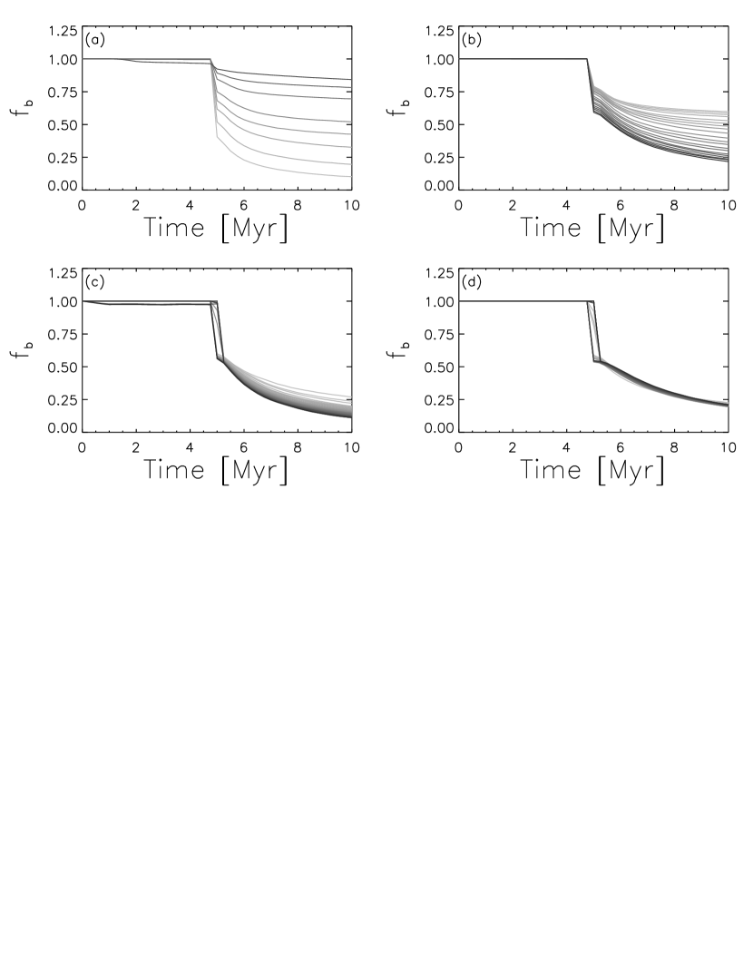
Figure 2: Fraction of stars $f_{b}$ that remain bound to the cluster’s gravitational potential as a function of time, for all of clusters included in the parameter space survey. Each panel corresponds to a different cluster parameter that is varied: (a) Star formation efficiency where $\varepsilon_{SF}$ ranges from $\varepsilon_{SF}=0.1$ (lower curve) to $\varepsilon_{SF}=0.75$ (upper curve) (b) Initial virial ratio where $Q_{i}$ ranges from $Q_{i}=0.025$ (upper curve) to $Q_{i}=0.5$ (lower curve), (c) Stellar Membership $N$ for scaling relationship $R_{c}\sim N^{1/2}$ where $N$ ranges from $N=100$ (upper curve) to $N=3000$ (lower curve), and (d) Stellar Membership $N$ for scaling relationship $R_{c}\sim N^{1/4}$ where $N$ ranges from $N=100$ to $N=3000$. The individual curves correspond to clusters with different initial values of the cluster parameter of interest. In all simulations the gas expulsion takes place at $t_{gas}=5~{}{\rm Myr}$. Immediately after gas removal, a significant fraction of stars become unbound from the cluster. As the cluster’s evolution continues, the mass loss rate drops significantly and $f_{b}$ approaches a constant value.

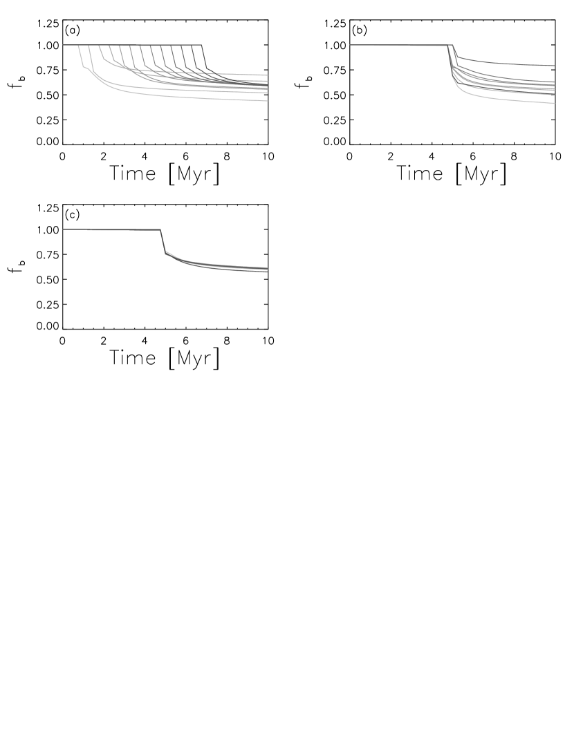
Figure 3: Continuation of Figure 2. Each panel corresponds to a different cluster parameter that is varied: (a) Gas removal time where $t_{gas}$ ranges from $t_{gas}=1$ Myr (lightest curve) to $t_{gas}=7$ Myr (darkest curve), (b) Cluster scaling radius where $R_{sc}$ ranges from $R_{sc}=0.33~{}{\rm pc}$ (lightest curve) to $R_{sc}=3~{}{\rm pc}$ (darkest curve) and (c) Degree of primordial mass segregation where $F_{seg}$ ranges from $F_{seg}=0.01$ (lower curve) to $F_{seg}=0.99$ (upper curve). The individual curves correspond to clusters with different initial values of the cluster parameter of interest. In all simulations (except those in panel (a)), the gas expulsion takes place at $t_{gas}=5~{}{\rm Myr}$. Immediately after gas removal, a significant fraction of stars become unbound from the cluster. As the cluster’s evolution continues, the mass loss rate drops significantly and $f_{b}$ approaches a constant value.

The value of the bound fraction at $t=10~{}{\rm Myr}$ provides one measure of how tightly bound a cluster remains after the embedding gas is removed. Figures 4 and 5 display the value of the bound fraction at $t=10~{}{\rm Myr}$ as a function of the initial cluster parameter values for the range of parameters considered in this survey. Previous theoretical and numerical work has identified a cluster’s star formation efficiency $\varepsilon_{SF}$ as the most important parameter in determining whether or not a cluster will remain gravitationally bound (Hills, 1980; Elmegreen, 1983; Lada et al., 1984). In clusters with high SFEs, a large proportion of the total cluster mass remains behind (in the form of stars) after the embedding gas is removed. Clusters with high SFEs remain more tightly bound after gas dispersal than clusters with low SFEs. In our cluster parameter survey, we also find that the bound fraction $f_{b}$ at $t=10~{}{\rm Myr}$ depends sensitively on the star formation efficiency $\varepsilon_{SF}$ of the cluster. Figure 4 panel (a) displays the cluster bound fraction $f_{b}$ as a function of star formation efficiency, $\varepsilon_{SF}$. The data is well fit by a power-law in $\varepsilon_{SF}$:

$$f_{b}=2.23\left(\varepsilon_{SF}\right)^{1.2}\qquad{\rm where}\qquad\varepsilon_{SF}\leq 0.5\,.$$ (5)

This fit is shown as the solid curve (line) in the figure.

Figure 4: Cluster bound fraction $f_{b}$ at $t=10~{}{\rm Myr}$ plotted as a function of cluster initial conditions, for all clusters included in the parameter space survey. The best fit functions described in the text are displayed in panels (a) – (d). The cluster parameter varied in each panel is as follows: (a) Star formation efficiency $\varepsilon_{SF}$, (b) Initial virial ratio $Q_{i}$, (c) Stellar Membership $N$ for scaling relationship $R_{c}\sim N^{1/2}$, (d) Stellar Membership $N$ for scaling relationship $R_{c}\sim N^{1/4}$. Different curves and circle sizes indicate different initial conditions within each series of simulations. In panels (a) and (b) $N=300,1000$, and $2000$ are indicated by the small, medium, and large circles, respectively, though there are no major differences between the clusters as a function of size. In panels (c) and (d), subvirial clusters are indicated by the solid curve while virial clusters are indicated by the dashed curve.

Figure 5: Continuation of Figure 4. The cluster parameter varied in each panel is as follows: (a) Gas removal time $t_{gas}$, (b) Cluster scaling radius $R_{sc}$, and (c) Degree of primordial mass segregation $F_{seg}$. Different curves and circle sizes indicate different initial conditions within each series of simulations. In panels (a), (b), and (c) $N=300,1000$, and $2000$ are indicated by the small, medium, and large circles connected by thin, medium, and thick curves, respectively. In panel (c) there are no major differences between the clusters as a function of size and the best fit function described in the text is displayed.

In the suite of simulations used to investigate the effects of star formation efficiency, the clusters are initially subvirial. After gas removal, subvirial clusters are more tightly bound than virial clusters (APFM). For even relatively high star formation efficiencies ($\varepsilon_{SF}=0.3$) and small initial virial parameters, conditions which produce the most tightly bound systems, the clusters are significantly disrupted by gas removal and promptly lose $\sim 40\%$ of their stars. Star formation efficiencies larger than $\sim 30\%$ are rarely observed (Lada & Lada, 2003, and references therein), and are difficult to attain theoretically (Matzner & McKee, 2000). Our results are thus in agreement with previous studies indicating that a significant fraction of the stellar population is lost from a cluster during the gas removal phase (e.g., Lada et al. 1984, Adams 2000, Boily & Kroupa 2003ab).

As mentioned above, clusters with subvirial initial velocities are more tightly bound than clusters with virial initial conditions. Figure 4 panel (b) demonstrates this trend by plotting the bound fraction as a function of the initial virial ratio. The bound fraction decreases steadily with the initial virial ratio $Q_{i}$ over the range considered, $0.01\leq Q_{i}\leq 0.5$. Gas removal has a weaker effect on spherical clusters with subvirial initial conditions because as a subvirial cluster collapses, more of the stars spend more of their time inside of the embedding gas (which is assumed to be static, i.e., not in a state of global collapse). When the embedding gas is removed from the cluster, many of the cluster members are interior to the gas and are less affected by the change in potential. The results from this suite of simulations again indicate that a significant fraction of cluster members are lost due to the change in the gravitational potential that occurs during the dispersal of the natal gas. In the most tightly bound subvirial clusters with $Q_{i}=0.025$, approximately $40\%$ of stars become unbound due to dispersal of the gas.

In clusters with subvirial initial conditions, the bound fraction remains constant as a function of cluster membership $N$, for both the $R_{c}\sim N^{1/2}$ and the $R_{c}\sim N^{1/4}$ cluster membership-radius scaling relations. This finding also holds true for virial clusters that have cluster membership-size relations similar to those observed in the solar neighborhood ($R_{c}\sim N^{1/2}$). The bound fraction at $t=10~{}{\rm Myr}$ is plotted as a function of cluster size $N$ in panels (c) and (d) of Figure 4. The upper curves in these panels indicate the bound fraction at $10~{}{\rm Myr}$ in the more tightly bound subvirial clusters, whereas the lower curves correspond to the virial clusters.

In virial clusters with a lower power-law index $\alpha$ in the cluster membership-size relation ($R_{c}\sim N^{1/4}$), the bound fraction decreases as a function of the cluster membership $N$. The bound fraction decreases roughly as $f_{b}\sim N^{-1/4}$ (see Figure 4, panel (c), lower curve). This decrease in $f_{b}(N)$ is due to a combination of effects arising from the relationship between cluster radius and cluster membership defined by equation (1). In clusters with $R_{c}\sim N^{1/4}$, the mean velocity and velocity dispersion scale approximately as $\left<v\right>\sim\sigma_{v}\sim\sqrt{GmN/R_{c}}\sim N^{3/8}$. The velocity distributions in the clusters are nearly Gaussian during the embedded phase (rather than perfectly Maxwellian as would be expected in a collisionless isothermal sphere of stars). As a result, the increased velocity dispersion in clusters with larger $N$ results in more stars with velocities high enough to escape from the cluster $v_{esc}\sim\sqrt{2GmN/R_{c}}$. In addition, the interaction rate between cluster members increases with the stellar density, which increases as $n\sim N^{1/4}$ in these clusters. In virial clusters with $R_{c}\sim N^{1/2}$ (Figure 4, panel (d), lower curve), the bound fraction is roughly constant. This trend occurs because although the average velocity and velocity dispersions increase as a function of cluster membership, the dependence on $N$ is not as strong: $\left<v\right>\sim\sigma_{v}\sim N^{1/4}$. In addition, the stellar density actually decreases with $N$, $n\sim N^{-1/2}$; the competing effects of increased velocities and lower interaction rates are comparable and act to cancel each other out.

The bound fraction does not appear to be simply related to either the gas removal timescale $t_{gas}$ or the scaling radius $R_{sc}$, i.e., the bound fraction $f_{b}$ is not a monotonic function (see Figure 5, panels (a) and (b)). This result occurs because in subvirial clusters, such as the ones considered in these parameter space surveys, changing either the scaling radius or the gas removal time affects the relationship between the gas removal time and the initial collapse and relaxation time. The resulting $f_{b}$ is sensitive to the particular dynamical state of the system at the time of gas removal. For example, if the cluster is re-expanding (after its initial collapse) when the gas is removed, many stars will have trajectories that are directed radially outward and are thus more likely to become gravitationally unbound.

Next, we consider the effects of primordial mass segregation. In general, the effects of mass segregation saturate when more than approximately $20\%$ of the stars are segregated by mass. Mass segregation only slightly affects the bound fraction, and clusters with minimal mass segregation (where the largest star is located at the cluster center) have slightly lower bound fractions than clusters with $F_{seg}=0.2$, as shown in panel (c) of Figure 5.

In summary, the results of this part of the study indicate that the star formation efficiency $\varepsilon_{SF}$ is the parameter that most significantly affects the fraction of a cluster that remains bound after the embedding gas is removed from the system. In addition, the initial virial state of the cluster, as well as the specific dynamical state at the time of gas dispersal, are important parameters in determining how many members remain bound to the cluster. We find that in sufficiently subvirial clusters, $Q_{i}\lesssim 0.2$, the bound fraction is not a sensitive function of the initial stellar density (as indicated by the suite of simulations varying $N$ and the cluster membership-radius relations), but rather is dominated by the fact that the initial global collapse produces a cluster whose members reside interior to the bulk of the embedding gas and thus are not strongly affected by the gas removal.

Two caveats should be included in this discussion. First, current observations of young emerging clusters cannot determine whether a cluster member is gravitationally bound or unbound from its host cluster. Over the first $\sim 10-20~{}{\rm Myr}$, bound and unbound clusters are visibly similar, and the results of simulations such as those presented here are not easily compared directly to observations. Second, this parameter space study focuses on the early evolution of embedded clusters. Additional dynamical evolution of the clusters on timescales greater than $\sim 10~{}{\rm Myr}$ will lead to even lower bound fractions $f_{b}$ at later times. As a result, the bound fractions presented in this work should be considered as upper limits on the expected bound fractions for clusters with older ages.

Finally we note that Tables 2 – 7 provide compilations of the bound fractions $f_{b}$ evaluated at time $t$ = 10 Myr for the simulations presented here. Each table lists the bound fractions $f_{b}$ as a function of a given input variable, including the stellar membership $N$ (Table 2), initial virial parameter $Q_{i}$ (Table 3), cluster scaling radius $R_{sc}$ (Table 4), star formation efficiency $\varepsilon_{SF}$ (Table 5), gas removal time $t_{gas}$ (Table 6), and the mass segregation parameter $F_{seg}$ (Table 7).

3.2 Stellar Interaction Rates

A significant consequence of living in high density environments, such as those found in young embedded clusters, is that close encounters with other cluster members may be relatively frequent. If these interactions are sufficiently close, they can have important ramifications for planet formation in circumstellar disks and for solar system survival. During early stages of solar system formation, encounters can disrupt protoplanetary disks and limit the mass reservoir for planet formation (Ostriker, 1994; Heller, 1993, 1995; Kobayashi & Ida, 2001). At later times, close encounters can disrupt planetary systems themselves, by significantly altering the eccentricities of planets and, in sufficiently close encounters, ejecting planets from the solar system entirely (Adams & Laughlin 2001, APFM).

Throughout the cluster simulations, close encounters with distance of closest approach less than $b=10^{4}$ AU are recorded. Note that the distance of closest approach is somewhat smaller than the impact parameter of the encounter due to gravitational focusing. A cumulative distribution of the close encounters is then constructed, and the interaction rate $\Gamma$ is calculated by averaging the encounter distributions over the time span of interest (here we use the embedded phase $t=0-t_{gas}$, the exposed phase $t=t_{gas}-10~{}{\rm Myr}$, or the entire $10~{}{\rm Myr}$ interval). Specifically, the interaction rate $\Gamma(b)$ is defined as the number of close encounters with distance of closest approach $r\leq b$ per star per million years. We find that the interaction rates have the form of power-laws for encounters with closest approach distances less than $\sim 3000$ AU. In other words, the interaction rate has the form

$$\Gamma=\Gamma_{0}\left(\frac{b}{1000\rm{AU}}\right)^{\gamma}\,,$$ (6)

where $b$ is the distance of closest approach. The fiducial interaction rate $\Gamma_{0}$ and the power-law index $\gamma$ are fit to the cumulative closest approach distribution for each set of cluster simulations. The fiducial interaction rate $\Gamma_{0}$ corresponds to the number of encounters with impact parameter $b$ less than $1000$ AU per star per million years. The fiducial interaction rate $\Gamma_{0}$ is displayed as a function of cluster initial conditions in Figures 6 and 7.

Figure 6: Fiducial interaction rate $\Gamma_{0}$ (in units of the number of interactions per star per Myr) is plotted as a function of initial cluster parameter, for all clusters included in the parameter space survey. The cluster parameter varied in each panel is as follows: (a) Stellar Membership $N$ for scaling relationship $R_{c}\sim N^{1/2}$, (b) Stellar Membership $N$ for scaling relationship $R_{c}\sim N^{1/4}$, and (c) Cluster scaling radius $R_{sc}$. Panel (d) displays the combined data from panels (a) - (c) as a function of initial stellar number density $n_{0}$ and displays the trend $\Gamma_{0}\sim n_{0}$ discussed in the text. In panels (a), (b), and (d) subvirial clusters are indicated by the solid curve while virial clusters are indicated by the dashed curve. In panel (c), clusters with $N=300,1000$, and $2000$ are indicated by the small, medium, and large circles (thin, medium, and thick curves), respectively.

Figure 7: Continuation of Figure 6. The cluster parameter varied in each panel is as follows: (a) Initial virial parameter $Q_{i}$, (b) Gas removal time $t_{gas}$, (c) Degree of primordial mass segregation $F_{seg}$, and (d) Star formation efficiency $\varepsilon_{SF}$. Clusters with $N=300,1000$, and $2000$ are indicated by the small, medium, and large circles (thin, medium, and thick curves), respectively.

Figure 8: The power-law index $\gamma$ for the interaction rates is plotted as a function of initial cluster parameter, for all clusters included in the parameter space survey. The cluster parameter varied in each panel is as follows: (a) Stellar Membership $N$ for scaling relationship $R_{c}\sim N^{1/2}$, (b) Stellar Membership $N$ for scaling relationship $R_{c}\sim N^{1/4}$, (c) Cluster scaling radius $R_{sc}$, and (d) Initial virial ratio $Q_{i}$. In panels (a) and (b), subvirial clusters are indicated by the solid curve while virial clusters are indicated by the dashed curve. In panels (c), and (d) clusters with $N=300,1000$, and $2000$ are indicated by the small, medium, and large circles (thin, medium, and thick curves), respectively.

Figure 9: Continuation of Figure 8. The cluster parameter varied in each panel is as follows: (a) Gas removal time $t_{gas}$, (b) Degree of primordial mass segregation $F_{seg}$, and (c) Star formation efficiency $\varepsilon_{SF}$. Clusters with $N=300,1000$, and $2000$ are indicated by the small, medium, and large circles (thin, medium, and thick curves), respectively.

For the parameter space considered in this study, the interaction rate $\Gamma$ depends most sensitively on a single parameter, the stellar number density $n$. The trends observed as a function of stellar membership $N$ and cluster scaling radius $R_{sc}$ (see Figure 6 panels (a) – (c)) are more fundamentally trends indicating how $\Gamma_{0}$ varies as a function of the average stellar density $n$ (keep in mind that the stellar density varies with $N$ and $R_{sc}$).

We can understand this behavior in simple terms as follows: Consider a cluster with $N$ stars and radius $R_{c}$. For simplicity, we ignore the difference between impact parameters and distances of closest approach $b$. A star passing through the cluster will experience, on average, a number $\delta n$ of close encounters with impact parameters within the range $b$ to $b+db$ (Binney & Tremaine, 1987), where $\delta n$ is given by

$$\delta n=\frac{2N}{R_{c}^{2}}b\delta b\,.$$ (7)

The crossing time in a cluster is given by $\tau_{c}\approx R_{c}/v$, where $v$ is the average stellar velocity. As a result, the star will experience close encounters in the given annulus at the rate

$$\delta\Gamma\approx\frac{2N}{R_{c}^{2}}\left(\frac{v}{R_{c}}\right)b~{}\delta b=2nvb~{}\delta b\,.$$ (8)

The interaction rate for all encounters with impact parameter less than $b$ is then given by $\Gamma\sim nvb^{2}$. Since the mean dynamical speeds are slowly varying over the regime of cluster parameter space considered in this paper, the interaction rate $\Gamma\propto n$ as claimed.

In Figure 6 panel (d), the $\Gamma_{0}$ values are plotted as a function of initial stellar density $n_{0}=N/R_{c}^{3}$ for all of the simulations with varying cluster membership $N$ and scaling radius $R_{c}$ (using the data from Figure 6 panels (a) – (c)). The plus symbols indicate the interaction rate $\Gamma_{0}$ for clusters with initially subvirial velocities, whereas the interaction rates for clusters with initially virial velocities are indicated by the x’s. Straight lines (indicating a power-law with index = $1$) are included in the panel; note that the numerically determined data are roughly consistent with the simple scaling relation $\Gamma_{0}\sim n_{0}$.

Figures 8 and 9 present the values of the index $\gamma$ that provide the best fit to the close encounter distributions as a function of the initial cluster parameters. The value of $\gamma$ does not vary strongly as a function of the initial conditions, but rather remains in the range $\sim 1-2$.

Using the simple argument constructed above, the total rate $\Gamma_{b}$ of close encounters with impact parameter less than $b$ in a cluster of membership size $N$ is given by

$$\Gamma_{b}\approx 0.122\,\,N^{-1/2}\left(\frac{b}{1000~{}{\rm AU}}\right)^{2}{\rm Myr}^{-1}\qquad{\rm for}\qquad R_{c}=1.0~{}{\rm pc}\left(\frac{N}{300}\right)^{1/2}\,,$$ (9)

and

$$\Gamma_{b}\approx 0.0095\,\,N^{1/4}\left(\frac{b}{1000~{}{\rm AU}}\right)^{2}{\rm Myr}^{-1}\qquad{\rm for}\qquad R_{c}=1.0~{}{\rm pc}\left(\frac{N}{300}\right)^{1/4}\,.$$ (10)

These estimates are similar to the interaction rates found for the virial clusters, although the fitted value of the index $\gamma$ is slightly lower than $2$ (due to gravitational focusing) in the numerically determined distributions (see Figures 8 and 9), and the fiducial interaction rate is somewhat higher.

The subvirial clusters have interaction rates that are about 8 times larger than the rates for virial clusters of the same starting density (as defined by $n_{0}\propto N/R_{c}^{3}$). This trend is due to a combination of the smaller effective cluster radius that a subvirial cluster attains after initially collapsing and its higher bound fraction after gas dispersal. During the embedded phase, subvirial clusters ($Q_{i}=0.04$) behave as if they have nearly zero-temperature starting states and thus collapse to roughly $\sqrt{2}$ of their initial size. This decrease in radius corresponds to an increase in density by a factor of $2\sqrt{2}$. In addition, subvirial clusters retain more of their members after the gas is removed from the cluster — we find that the bound fraction is $\sim 3$ times higher for the subvirial starting states. Since the close encounter profiles are averaged over the initial number of stars in the cluster, the interaction rates in subvirial clusters will be roughly 3 times higher than in virial clusters over the exposed phase of cluster evolution (due to increased stellar retention). Note that combining these two factors increases the interaction rates by $\sim 6\sqrt{2}\sim 8$. The results of the parameter survey varying $Q_{i}$ also indicate that subvirial clusters have higher interaction rates. In Figure 7 panel (a), the interaction rate clearly decreases as a function of initial virial parameter $Q_{i}$.

We also find that the interaction rates are somewhat higher in clusters that have more of their massive stars residing near the cluster center (see Figure 7, panel (c)). This finding is consistent with the modeling results of the observed cluster NGC 1333 presented in APFM. The fiducial interaction rate $\Gamma_{0}$ in the simulated NGC 1333 cluster was approximately $5$ times higher than the $\Gamma_{0}$ calculated in equivalent subvirial clusters with minimal mass segregation. We suggested that the increased interaction rate was due to the primordial mass segregation observed in NGC 1333 (see Figure 15 of APFM). For comparison, subvirial clusters with $N$ = 300 stars and $F_{seg}=0.05$ have fiducial interaction rates that are about $5$ times larger than those found in subvirial clusters with $N=300$ members and minimal mass segregation (see Figure 7, panel (c), top curve).

The average interaction rate also increases as a function of gas removal time $t_{gas}$ as shown in Figure 7 panel (b). This interaction rate is averaged over the $10~{}{\rm Myr}$ simulation time. However, the majority of close encounters occur during the embedded phase, and hence the average interaction rate increases as the length of the embedded phase increases. For clusters with embedded phases lasting more than $\sim 2~{}{\rm Myr}$, the rate of close encounters during the embedded phase is roughly constant. When the embedded phase lasts less than $\sim 2~{}{\rm Myr}$, the clusters have lower encounter rates due to lower densities during the first $\sim 1~{}{\rm Myr}$ while the subvirial cluster is still contracting. For completeness, we note that the interaction rate does not display strong trends with varying star-formation efficiency $\varepsilon_{SF}$ (see Figure 7, panel (d)).

For all of the simulations discussed in this section, Tables 8 – 13 provide listings of the parameters ($\Gamma_{0}$, $\gamma$) that specify the interaction rates through equation (6). Each table provides the values of $\Gamma_{0}$ and $\gamma$ as a function of a given input variable, including the stellar membership $N$ (Table 8), initial virial parameter $Q_{i}$ (Table 9), cluster scaling radius $R_{sc}$ (Table 10), star formation efficiency $\varepsilon_{SF}$ (Table 11), gas removal time $t_{gas}$ (Table 12), and the mass segregation parameter $F_{seg}$ (Table 13). These interaction rates, as determined by the values of $(\Gamma_{0},\gamma)$, are one of the primary products of this investigation. They can be used to calculate interaction rates as a function of closest approach distance for a wide variety of cluster environments (see Section 4.1 below for one such application).

3.3 Interaction Velocities

In addition to constructing the distribution of closest approach distances associated with close encounters in the simulated clusters, we also determine the distribution of encounter velocities. The distribution of encounter velocities provides additional information regarding the effect that close encounters may have on the constituent solar systems. For example, the interaction cross sections depend on the encounter speeds.

We define the encounter velocity $v_{enc}$ as the magnitude of the relative velocities of the stars at the moment of closest approach. We then create distributions of the frequency of encounter velocities throughout the simulations. Figure 10 presents the resulting distribution of encounter velocities for a cluster with radius $R_{c}=1~{}{\rm pc}$, $N=300$ stars, and subvirial initial speeds ($Q_{i}=0.04$). A binning size of $0.25~{}{\rm km~{}s}^{-1}$ has been used to construct the histogram, and error bars are included on the distribution to indicate the dispersion within each velocity bin.

Figure 10: The distribution of interaction velocities in a subvirial cluster with $N=300$, $R_{c}\sim N^{1/2}$, and $Q_{i}=0.04$. The distribution averaged over the interval $t=0-10~{}{\rm Myr}$ is presented in panel (a). Panel (b) displays the time averaged distribution of interaction velocities during the embedded phase ($t=0-5~{}{\rm Myr}$) and panel (c) presents the distribution averaged over the remainder of the cluster evolution ($t=5-10~{}{\rm Myr}$). The histogram binning size is $0.25~{}{\rm km~{}s}^{-1}$. Error bars correspond to the dispersion (variance) within each velocity bin. The best fit Gaussian curve is indicated by the dashed curve, and the mean of the Gaussian is indicated by the vertical dash-dot line.

We find that the encounter velocity distribution can be approximated reasonably well by a Gaussian curve where the mean and the width (as measured by the variance $\sigma^{2}$) of the Gaussian are varied to fit the encounter velocity distribution for each particular set of initial conditions. The Gaussian fits to the velocity distributions in Figure 10 are indicated by the dashed curves. We note that the Gaussian fit slightly overestimates the number of low velocity encounters with $v_{enc}\lesssim 0.5~{}{\rm km~{}s}^{-1}$ (and formally even predicts a few encounters with negative velocities). However, the general shape and width of the distribution are well represented by these gaussian forms.

In Figures 11 and 12, the mean encounter velocity $\left<v_{enc}\right>$ is plotted as a function of the initial cluster parameter. The encounter velocity has been normalized by the mean velocity within the cluster’s half-mass radius (the regime where most of the interactions occur within the cluster). The error bars indicate the normalized width (FWHM) of the Gaussian that best fits the velocity distribution. This figure demonstrates that the normalized encounter velocity distributions do not vary strongly as a function of the initial conditions, but rather are a robust function of mean cluster velocity.

The encounter velocities are about twice the average velocity in the interactive region of the cluster. This result is roughly consistent with an analytic estimate of the relative velocities of cluster members whose velocities are sampled from a Maxwellian distribution, so that $\sqrt{v_{rel}^{2}}\sim\sqrt{2\left<v^{2}\right>}$ (Binney & Tremaine, 1987). The encounter velocities are somewhat larger than those predicted by this estimate (about twice the mean velocity) due in part to gravitational focusing. Note that $b\sim 10^{3}$ AU is a typical encounter distance, and that the orbit speed $v_{\rm orb}\sim(GM_{\ast}/b)^{1/2}\sim 1$ km s^-1, so that the gravity of the stars taking part in the encounter does matter. The numerically calculated distribution of interaction velocities includes only a subsample of the relative velocities, because only encounters with impact parameter $b\lesssim 10^{4}$ AU are included in the interaction velocity distribution, and this subsample is likely to have somewhat larger relative velocities.

Figure 11: The parameters specifying the distribution of interaction velocities, specifically the mean $\mu$ and the FWHM of the distribution as a function of initial cluster parameter, for all clusters included in the parameter space survey. The mean interaction velocity $\mu$ (in ${\rm km~{}s}^{-1}$) is indicated by the data points and the FWHM is depicted by the error bars. Velocities are scaled by the cluster mean velocity. The distribution parameters $\mu$ and FWHM are presented as a function of (a) Stellar membership $N$ for virial clusters $Q_{i}=0.5$ and $R_{c}\sim N^{1/2}$, (b) Stellar membership $N$ for subvirial clusters $Q_{i}=0.04$ and $R_{c}\sim N^{1/2}$, (c) Initial cluster scaling radius $R_{sc}$, and (d) Star formation efficiency $\varepsilon_{SF}$.

Figure 12: Continuation of Figure 11. The distribution parameters $\mu$ and FWHM are presented as a function of (a) Initial virial parameter $Q_{i}$, (b) Time of gas removal $t_{gas}$, and (c) Degree of primordial mass segregation $F_{seg}$.

3.4 Mass and Number Distributions

As a cluster evolves, interactions between stars, and between the stars and the background gas potential, produce a distribution of stellar positions and velocities. The distribution of stars within a cluster at a given time $t$ can be characterized by the cumulative mass distribution $M(r,t)/M_{T\ast}$ or the cumulative number distribution $N(r,t)/N$, where $M_{T\ast}$ and $N$ are the total masses and numbers of the stars that are gravitationally bound to the cluster at time $t$, respectively. In the simulated clusters, each of these distributions is calculated at intervals of $0.25$ Myr. The profiles are then averaged over the cluster lifetime and over 100 realizations of the cluster used to produce a statistical description of the mass and number profiles. We find that both of these distributions may be fit by simple functions of the form

$$\frac{M(r)}{M_{T\ast}}=\left(\frac{\xi^{a}}{1+\xi^{a}}\right)^{p},$$ (11)

$$\frac{N(r)}{N}=\left(\frac{\xi^{a}}{1+\xi^{a}}\right)^{p},$$ (12)

where $\xi=r/r_{0}$ and the scale radius $r_{0}$ and index $p$ are free parameters that are fit to the distributions observed in the simulated clusters. The parameter $a$ may also be varied to fit the data. We find that the choice $a=2$ gives the best fit for the subvirial clusters and $a=3$ gives the best fit for the initially virial clusters (this finding is consistent with the results found in APFM). In the series of simulations where the initial virial parameter $Q_{i}$ is varied, the choice $a=2$ works best for simulations for which $Q_{i}<0.25$, and $a=3$ works best for those with $Q_{i}\geq 0.25$. The parameters $r_{0}$ and $p$ that provide the best fit for the radial distributions (equation [12]) and the mass profiles (equation [11]) are similar, although not identical, because stars of different masses have somewhat different radial profiles.

These radial profiles of clusters provide insight into the general evolution of a cluster, and perhaps more importantly, into the expected radiation fields that young solar systems in the cluster will experience. Circumstellar disks and forming solar systems residing in a cluster will be subjected to the FUV and EUV radiation fields produced by the cluster population, and these fields are dominated by the large stars in the cluster. If these radiation fields are strong enough, they are capable of photoevaporating circumstellar disks and thereby preventing (or at least limiting) giant planet formation. The massive young stars that produce the majority of the UV radiation are often located near the center of the cluster (Hillenbrand & Hartmann, 1998; Bonnell & Davies, 1998; Lada & Lada, 2003). To first approximation, the UV radiation is a cluster can be considered as a point source at the center. An understanding of the EUV and FUV fields associated with young clusters combined with the average radial distributions of stars in young clusters thus provides a framework with which to predict how effectively cluster radiation can restrict planet formation (Johnstone et al., 1998; Fatuzzo & Adams, 2008).

Figure 13: The median radius calculated from the radial profiles $N(r)/N$ as a function of initial cluster parameter, for all clusters included in the parameter space survey. The cluster parameter varied in each panel is as follows: (a) Initial virial ratio $Q_{i}$, (b) Gas removal time $t_{gas}$, (c) Stellar Membership $N$ for scaling relationship $R_{c}\sim N^{1/2}$, and (d) Stellar Membership $N$ for scaling relationship $R_{c}\sim N^{1/4}$. In panels (a) and (b) clusters with $N=300,1000$, and $2000$ are indicated by the small, medium, and large circles (thin, medium, and thick curves), respectively. In panels (c) and (d), subvirial clusters are indicated by the solid curve while virial clusters are indicated by the dashed curve.

Figure 14: Continuation of Figure 13. The cluster parameter varied in each panel is as follows: (a) Cluster scaling radius $R_{sc}$, (b) Star formation efficiency $\varepsilon_{SF}$, and (c) Degree of primordial mass segregation $F_{seg}$. Clusters with $N$ = 300, 1000, and 2000 are indicated by the small, medium, and large circles (thin, medium, and thick curves), respectively.

Figure 15: The median radius calculated from the radial profiles $N(r)/N$ normalized by the initial cluster radius $R_{c}$ as a function of initial cluster parameter, for all clusters included in the parameter space survey. The cluster parameter varied in each panel is as follows: (a) Initial virial ratio $Q_{i}$, (b) Gas removal time $t_{gas}$, (c) Stellar Membership $N$ for scaling relationship $R_{c}\sim N^{1/2}$, and (d) Stellar Membership $N$ for scaling relationship $R_{c}\sim N^{1/4}$. In panels (a) and (b) clusters with $N=300,1000$, and $2000$ are indicated by the small, medium, and large circles (thin, medium, and thick curves); in panel (b), the dashed curves (marked by open triangles) show the result for the normalized median radius averaged over the embedded phase only. In panels (c) and (d), subvirial clusters are indicated by the solid curves while virial clusters are indicated by the dashed curves.

Figure 16: Continuation of Figure 15. The cluster parameter varied in each panel is as follows: (a) Cluster scaling radius $R_{sc}$, (b) Star formation efficiency $\varepsilon_{SF}$, and (c) Degree of primordial mass segregation $F_{seg}$. Clusters with $N$ = 300, 1000, and 2000 are indicated by the small, medium, and large circles (thin, medium, and thick curves), respectively, though there are no major differences between the clusters as a function of size.

Although one can use the full distributions (see equations [11, 12]), it is sometimes useful to characterize the distributions in terms of a single parameter. Toward this end, Figures 13 and 14 present the median cluster radius $r_{med}$ calculated from the fits to the cumulative radial distributions for the entire parameter space. The scale $r_{med}$ is defined as the radius at which $N(r)/N=0.5$ and thus represents the radius which, on average, contains half of the cluster members. As these plots indicate, the median cluster radius $r_{med}$ scales with the initial virial parameter $Q_{i}$, the gas removal timescale $t_{gas}$, the cluster membership $N$, and the cluster scaling radius $R_{sc}$. On the other hand, the radius $r_{med}$ does not vary strongly with the either star formation efficiency $\varepsilon_{SF}$ or the degree of primordial mass segregation $F_{seg}$.

Scaling the median radius $r_{med}$ by the initial cluster radius $R_{c}$ removes the dependency on this initial cluster parameter and more readily identifies trends that are distinct from the initial assumptions concerning cluster size. Figure 15 displays the median radius $r_{med}$ normalized by the initial cluster radius $R_{c}$. Panel (a) of this figure clearly shows that the median radius depends almost linearly on the initial virial parameter $Q_{i}$ for $Q_{i}\leq 0.5$. This result is consistent with what we expect from the initial collapse associated with the evolution of a cluster with subvirial velocities: The quasi-equilibrium radius (that obtained after the initial dynamical adjustment) scales linearly with the initial virial parameter. Clusters with completely subvirial starting states have median radii that are approximately $\sqrt{2}$ of the median radii of virial clusters.

The median radius also decreases as a function of the gas removal time $t_{gas}$. The data points connected by a solid line in Figure 15 panel (b) correspond to the time averaged (over $0-10$ Myr) normalized median radius $r_{med}$ of clusters with differing values of $t_{gas}$. During the embedded phase, these (initially subvirial) clusters remain bound and do not expand. As a result, clusters that become unbound early in their history have larger median radii simply due to time averaging (over the $10$ Myr time interval of the simulations). The data points connected by the dashed curve correspond to the normalized median radius averaged over the embedded stage of the cluster evolution ($0-t_{gas}$ Myr). Removing the apparent dependence on $t_{gas}$ that is actually due to the time averaging, we find that in clusters with dispersal times greater than $\sim 2$ Myr, the cluster median radius does not depend sensitively on the gas removal time $t_{gas}$.

Note that clusters with early gas dispersal times ($t_{gas}\lesssim 2$ Myr) have significantly larger median radii than clusters with later gas dispersal times. The average crossing time in a subvirial cluster is $\sim 1$ Myr, and thus gas removal within the first couple crossing times prevents the cluster from approaching a state of virial equilibrium. This behavior also explains why the bound fractions in clusters with $t_{gas}\lesssim 2$ Myr are very low (see Figure 5 panel (a), and the discussion in Section 3.1). In other words, the process of gas dispersal in a cluster that is not in virial equilibrium is more destructive to the cluster than if gas removal occurs after the system approaches an equilibrium state (Goodwin & Bastian, 2006).

Panel (a) in Figure 16 displays the normalized median cluster radius as a function of the initial scaling radius $R_{sc}$ used in equation (1). The normalization of the median cluster radius includes the intrinsic dependence on $R_{sc}$, and hence the trend observed in the normalized median radius $r_{med}/R_{c}$ must be accounted for by another mechanism. The larger normalized median radius observed in clusters with smaller initial values of $R_{sc}$ can be understood in terms of the higher interaction rates observed in these clusters; the interactions keep the cluster cores slightly inflated. This trend should be present, to some extent, in all clusters with high interaction rates; however, it is easiest to observe in the $R_{sc}$ series of simulations because the interaction rates have the widest dynamical range, varying by three orders of magnitude (see Figure 6, panel (c)).

Tables 14 – 19 list the values of the parameters $(p,r_{0},a)$ that specify the mass and number profiles for the clusters considered herein, where the profiles have the form given by equations (11) and (12). Each table lists the fitted parameters as a function of a given input variable, including the stellar membership $N$ (Table 14), initial virial parameter $Q_{i}$ (Table 15), cluster scaling radius $R_{sc}$ (Table 16), star formation efficiency $\varepsilon_{SF}$ (Table 17), gas removal time $t_{gas}$ (Table 18), and the mass segregation parameter $F_{seg}$ (Table 19). These tabulated values, in conjunction with equations (11) and (12), provide analytic descriptions of the mass and number density distributions for a wide variety of clusters. These analytic forms, in turn, can be used to calculate related physical quantities. For example, the cluster median radius $r_{med}$ is given by the formula

$$r_{med}=r_{0}\left(2^{1/p}-1\right)^{-1/a}\,,$$ (13)

where $(p,r_{0},a)$ are the parameters that specify the number density profile. As another example, the mass density of the cluster is given by

$$\rho(r)=\frac{1}{4\pi r^{2}}\frac{dM}{dr}=\frac{M_{T\ast}}{4\pi r^{3}}\frac{ap\,\xi^{ap}}{(1+\xi^{a})^{p+1}}\,=\frac{M(r)}{4\pi r^{3}}\frac{ap}{1+\xi^{a}}\,,$$ (14)

where the parameters $(p,r_{0},a)$ are those of the mass profile. Similarly, the magnitude of the gravitational force is given by $|F|=GM(r)/r^{2}$, and the corresponding potential of the stellar component can be obtained from the integral $\Psi_{\ast}\sim\int Fdr$. Note that the force can be expressed in terms of elementary functions, but the potential integral leads to hypergeometric functions for general values of the indices. These analytic forms can be used in a wide variety of applications to help determine the effects of cluster environments on forming stars and young solar systems.

4 Effects of Cluster Environment on Planetary Formation

In this section, we consider two mechanisms through which young embedded clusters affect their constituent members. Note that for systems in the regime of parameter space considered here, the background cluster environment has more effect on circumstellar disks and planet formation than on the star formation process itself. In Section 4.1, we use the interaction rates calculated from our ensemble of $N$-body simulations (Section 3.2) to determine the effectiveness of close encounters for disrupting circumstellar disks and newly formed planetary systems. In Section 4.2, we use the output number density profiles (from Section 3.4) to determine how much UV radiation the cluster provides to the circumstellar disks surrounding its members.

4.1 Close Encounters

One way that planet formation may be compromised in stellar clusters is through close encounters between planet-forming circumstellar disks and other cluster members. A close encounter will truncate a circumstellar disk down to a radius that is roughly $1/3$ the distance of closest approach (Kobayashi & Ida, 2001). We thus need a metric to determine the importance of close encounters during the 10 Myr embedded phase of cluster evolution (note that this timescale is comparable to the observed lifetimes of circumstellar disks and the expected time required for giant planet formation). Using data from our cluster simulations, we define the characteristic impact parameter $b_{C}$ as the closest encounter that an average star will experience over the course of a given time interval, taken here to be $10~{}{\rm Myr}$. The value of $b_{C}$ is readily calculated from the distribution of interaction rates. For the form given in equation (6), and we define the characteristic radius $b_{C}$ to be

$$b_{C}\equiv 1000\rm{AU}\left(t_{0}\Gamma_{0}\right)^{1/\gamma}\,,$$ (15)

where $t_{0}$ = 10 Myr.

Figure 17: The characteristic impact parameter, $b_{C}$ (in AU) calculated from the close encounter profiles $\Gamma$ plotted as a function of cluster parameter, for all clusters included in the parameter space survey. The cluster parameter varied in each panel is as follows: (a) Stellar Membership $N$ for scaling relationship $R_{c}\sim N^{1/2}$, (b) Stellar Membership $N$ for scaling relationship $R_{c}\sim N^{1/4}$, (c) Cluster scaling radius $R_{sc}$, and (d) Initial virial ratio $Q_{i}$. In panels (a) and (b), subvirial clusters are indicated by the solid curve while virial clusters are indicated by the dashed curve. In panels (c) and (d) clusters with $N=300,1000$, and $2000$ are indicated by the small, medium, and large circles (thin, medium, and thick curves), respectively. The dashed (solid) horizontal lines correspond to benchmark distances of 190 AU (120 AU).

Figure 18: Continuation of Figure 17. The cluster parameter varied in each panel is as follows: (a) Gas removal time $t_{gas}$, (b) Degree of primordial mass segregation $F_{seg}$, and (c) Star formation efficiency $\varepsilon_{SF}$. Clusters with $N=300,1000$, and $2000$ are indicated by the small, medium, and large circles (thin, medium, and thick curves), respectively. The dashed (solid) horizontal lines correspond to benchmark distances of 190 AU (120 AU).

Figures 17 and 18 display the characteristic impact parameter $b_{C}$ as a function of initial cluster parameter for the clusters considered in this parameter space survey. The horizontal dashed and solid lines (at $190$ AU and $120$ AU) indicate encounter distances that restrict planet formation in a circumstellar disk to distances less than $55$ AU and $30$ AU, respectively (Kobayashi & Ida, 2001). These latter distances correspond to the outer edge of the Kuiper Belt and the orbit of the planet Neptune in our solar system.

These figures indicate that most of the clusters in this parameter space survey do not have interaction rates that are high enough to seriously compromise planet formation within the $55$ AU Kuiper Belt radius, or even within $100$ AU. Equivalently, disruptive encounters at these close distances are predicted to be rare. In the most interactive clusters, those with the highest number densities due to small values of $R_{sc}$ (Figure 17, panel (c)), and those with significant amounts of mass segregation (Figure 18, panel (b)), the characteristic scale $b_{C}$ is small enough that planet-forming disks may be truncated at radii $r_{d}\lesssim 100$ AU and hence giant planet formation in this class of clusters can be partially inhibited. Nonetheless, the cluster environment provides only moderate constraints on the planet forming process.

Interactions remain important even after planet formation in the circumstellar disk has taken place. Close encounters with other cluster members are capable of disrupting newly formed planetary systems. In this context, the primary channel of “disruption” is to increase the orbital eccentricity and/or the inclination angles of the planetary orbits. Sufficiently close encounters can eject planets from their orbits entirely, and produce free floating planets in the clusters. The stellar interaction rates presented in this paper may be combined with scattering calculations to investigate the rate of solar system disruption in young clusters.

One way to characterize the possible effects of clusters on newly formed planetary systems is to pose the following question: Under the assumption that planet formation naturally produces systems similar to our solar system (with planets in relatively circular orbits with small inclination angles), how many planetary systems in a young cluster will be noticeably different due to an encounter with another cluster member? Previous work provides cross sections for disrupting solar systems in a variety of ways (e.g., Adams & Laughlin 2001, APFM); as expected, scattering interactions are most effective at altering the orbits of the outermost planets. For the sake of definiteness, we consider a collection of solar systems that have the same architecture as our own (same masses and semimajor axes for the outer planets) except that the orbits are circular. We then designate a solar system to be “noticeably different” (due to an encounter) when the analog of Neptune has its orbital eccentricity increased (from zero) to values $\epsilon\geq 0.05$ (about twice the value observed in our solar system). We note that nothing especially dramatic happens when orbital eccentricities are increased by this amount, only that the solar system is changed enough to be noticed. Previous work shows that the cross section for increasing Neptune’s eccentricity to $\epsilon\geq 0.05$ during an encounter with a cluster member is $\langle\sigma\rangle\approx$ 167,000 AU² (Adams & Laughlin, 2001), which corresponds to a closest approach distance of approximately 230 AU. This cross section for increasing Neptune’s eccentricity is about the same as the cross section for increasing the spread in inclination angles beyond that observed in our solar system ($\Delta i\geq 3.5^{\circ}$). For completeness, we note that in these solar system scattering calculations, the perturber is assumed to be a binary star system, which is reasonable since a large fraction of stars are members of multiple systems.

As shown in Figures 17 and 18, the typical interaction distance $b_{C}$ is somewhat larger than the $230$ AU encounter distance required to “disrupt” the solar system. However, some fraction of stars in a cluster will experience encounters that are significantly closer. For instance, consider a cluster with $N$ = 300 stars, subvirial initial conditions characterized by $Q_{i}$ = 0.04, and an initial cluster radius $R_{c}=0.67$ pc. In this cluster, $b_{c}\approx 400$ (see Figure 17, panel (c)). The rate of interactions with an encounter distance less than or equal to $b$ can be determined from equation (6) using the values $\Gamma_{0}$ = 0.333 and $\gamma=1.47$. The rate of close encounters with $b\leq 230$ AU is thus about $0.038$ interactions per star per Myr. As a result, in this cluster approximately 115 stars will experience close encounters severe enough to change their planetary systems. In contrast, in a cluster similar in all respects except with a slightly larger initial radius (i.e., $N=300$, $Q_{i}=0.04$, and $R_{c}1$ pc), this number drops to $\sim 50$ planetary systems ($\Gamma_{0}=0.1290,\gamma=1.39$).

This example illustrates the type of calculations that are possible using the interaction rates and fitting parameters presented in this numerical study. The close encounter distributions may also be combined with results presented by other scattering calculations to determine the efficacy of circumstellar disk and planetary system disruption in young stellar clusters (Heller, 1993, 1995; de La Fuente Marcos & de La Fuente Marcos, 1997, 1999; Kobayashi & Ida, 2001; Adams & Laughlin, 2001; Adams et al., 2006; Pfalzner, 2008).

Before leaving this section, we can use the interaction rates determined here to provide a consistency check. Although this ensemble of simulations does not include binary systems (only single stars), the presence of binaries could affect the energy budget of the system. As outlined above, relatively few stellar interactions take place with distances of closest approach less than 100 AU, and the characteristic radii $b_{C}$ are typically much larger ($\sim 1000$ AU). For comparison, for solar type stars, the peak of the binary period distribution occurs at a period $P\approx 10^{5}$ days (Duquennoy & Mayor 1991), which corresponds to a distance of $\sim 40$ AU. As a result, the closest encounter experienced by the the vast majority of stars (during the 10 Myr window of interest) is much wider than the typical binary separation. These results thus vindicate the approach of ignoring binarity for this class of simulations. However, we note that for more extreme regimes of parameters space (e.g., dense stellar systems destined to become globular clusters), neglecting binaries is not a good approximation.

4.2 Radiation Fields

Another mechanism through which cluster environments may affect planet formation is by photoevaporation of protoplanetary disks due to the enhanced FUV radiation fields produced by massive young stars. It is well known that radiation from the central host star can heat and dissipate its surrounding planet-forming disk (Shu et al., 1993; Hollenbach et al., 1994). Most stars are not massive enough to produce large quantities of FUV radiation, the wavelength range that most effectively photoevaporates the disk. In young clusters, however, the most massive cluster stars can provide FUV radiation fields that are strong enough to photoevaporate the disks associated with other cluster members (Johnstone et al., 1998; Adams & Myers, 2001) and dominate over the radiation produced by the host star.

Recent studies have determined the FUV (and EUV) luminosities of clusters as a function of cluster membership $N$, the mass function of the cluster, and various amounts of extinction within the cluster (e.g., Armitage 2000, APFM, Fatuzzo & Adams 2008). In this section, we combine these previous determinations of the typical FUV background luminosities in stellar clusters with the radial profiles presented in Section 3.4. Taken together, these stellar positions and the FUV luminosities determine the expected FUV flux that impinges upon the circumstellar disks in young stellar clusters. In these systems, this FUV flux places limits on both the timescale over which planets may form and the region of the disk that has the potential to form planets.

The total FUV luminosity of a cluster originates primarily from the most massive stars in the cluster. As a result, the cluster FUV luminosity is sensitive to the membership size $N$ of the cluster and the mass function of the stars in the cluster. APFM presented detailed calculations of the expected FUV luminosity in a cluster of size $N$ (see their Figure 6). For each cluster membership size $N$, the distribution of possible FUV luminosities is quite wide due to under-sampling of the stellar initial mass function; for clusters with $N\lesssim 700$, the width of the FUV luminosity distribution is larger than the mean (or median) value. As a result, clusters are predicted to display substantial system to system variation in the radiation fields they produce (especially for $N\lesssim$ 700).

Each individual cluster member will experience a FUV flux that is time-dependent as it orbits through the cluster potential. For purposes of this paper, we estimate the typical flux experienced by a circumstellar disk in a simulated cluster by combining the FUV luminosity $L_{\rm FUV}(N)$ with the median radial position of the stars in a simulated cluster. The vast majority of the FUV radiation in a cluster is produced by the most massive stars, which typically reside near the cluster’s center (see Section 2.2.6). The FUV source is thus modeled as a point source at the center of the cluster. For a given cluster with FUV luminosity $L_{\rm FUV}(N)$ and median radius $r_{med}$, the corresponding median FUV flux ${\cal F}_{\rm FUV}$ experienced by the protoplanetary disks in the cluster is defined to be

$${\cal F}_{\rm FUV}\equiv\frac{L_{\rm FUV}(N)}{4\pi r_{med}^{2}}\,,$$ (16)

where $r_{med}$ is defined by the radial probability distribution of the cluster (equation [12]) and $L_{\rm FUV}(N)$ is taken from the results presented in APFM.

In addition to the FUV flux provided by the background cluster, a circumstellar disk is also subjected to FUV radiation from its host star. Observations of T Tauri stars provide estimates of the FUV flux experienced by their disks at distances of $\sim 100$ AU due to the central star (Bergin et al., 2004). For three T Tauri stars, these authors determine FUV fluxes of $G_{0}$ = 240, 340, and 1500 where $G_{0}=1$ corresponds to a benchmark value of $1.6\times 10^{-3}$  erg s^-1 cm^-2 (close to the value of the interstellar radiation field at FUV wavelengths). As a rough estimate, the FUV flux associated with the host star can be taken to be $G_{\rm host}\approx 500$. When the background FUV radiation field of the cluster exceeds this benchmark value, the environment can, in principle, affect the evolution of circumstellar disks and planet formation. However, in the outer regions of a cluster, where flux levels from the central massive stars are relatively low, the FUV flux from the host star can be more important than the FUV flux from the background cluster.

Figures 19 and 20 present the median cluster FUV flux ${\cal F}_{\rm FUV}$ (defined by equation [16]) as a function of the initial cluster parameters for the clusters considered in this parameter space survey. The dashed horizontal lines correspond to FUV radiation levels of $G_{0}$ = 300 and 3000, values for which the effects of photoevaporation on circumstellar disks have been calculated in detail (Adams et al., 2004). The results of these photoevaporation models provide a rough scaling law: Over the course of $10$ Myr, an FUV flux of $G_{0}=3000$ is capable of truncating a circumstellar disk down to a radius $r_{d}$ given by

$$r_{d}\approx 36~{}{\rm AU}\left(\frac{M_{\ast}}{\rm M_{\odot}}\right)\,,$$ (17)

where the result depends on the stellar mass $M_{\ast}$. This nominal radius is close to the size of our solar system. As a rough rule of thumb, significant evaporation around solar type stars thus requires flux levels $G_{0}\gtrsim 3000$, with a weaker requirement for smaller stars.

Figure 19: The FUV flux experienced due to the cluster environment for all clusters included in the parameter space survey. The cluster parameter varied in each panel is as follows: (a) Initial virial ratio $Q_{i}$, (b) Gas removal time $t_{gas}$, (c) Stellar Membership $N$ for scaling relationship $R_{c}\sim N^{1/2}$, and (d) Stellar Membership $N$ for scaling relationship $R_{c}\sim N^{1/4}$. In panels (a) and (b) clusters with $N=300,1000$, and $2000$ are indicated by the small, medium, and large circles (thin, medium, and thick curves), respectively. In panels (c) and (d), subvirial clusters are indicated by the solid curve while virial clusters are indicated by the dashed curve. The horizontal lines at $G_{0}=300$ and $3000$ are benchmark values for which the effects of photoevaporation of circumstellar disks have been calculated (Adams et al., 2004).

Figure 20: Continuation of Figure 19. The cluster parameter varied in each panel is as follows: (a) Cluster scaling radius $R_{sc}$, (b) Degree of primordial mass segregation $F_{seg}$, and (c) Star formation efficiency $\varepsilon_{SF}$. Clusters with $N$ = 300, 1000, and 2000 are indicated by the small, medium, and large circles (thin, medium, and thick curves), respectively.

The FUV luminosity of a cluster is an increasing function of the cluster membership $N$, and this trend is visible in the FUV fluxes shown in Figures 19 and 20. In subvirial clusters with more than $N\sim 1000$ members, circumstellar disks are exposed to median FUV fluxes that are of order $G_{0}\approx 3000$ (see Figure 19, panels (c) and (d)). In this class of clusters, significant photoevaporation of the outer disk is predicted to take place. Many of the circumstellar disks in such cluster systems will be truncated, so that planet formation is limited to the inner $\sim 35$ AU for solar type stars. For the more numerous red dwarf stars, planet formation is limited to the inner $\sim 12$ AU. In clusters with smaller memberships $N$, the radiation fields are more modest and disks will not be significantly photoevaporated by cluster radiation. We note that in this latter class of clusters, the FUV radiation from the host star is comparable to that of the background cluster. Finally, we note that in clusters where gas expulsion takes place on short time scales ($t_{gas}\leq$ 3 Myr), the FUV fluxes are lower due to early expansion of the cluster and larger values of $r_{med}$ (see panel (b) of Figure 19).

5 Conclusion

In this paper, we have presented the results from a large ensemble of numerical simulations designed to study the dynamics young embedded clusters over a wide range of conditions. The choice of parameter space was motivated by recent catalogs and surveys of star-forming environments in the solar neighborhood. We consider clusters with a range of stellar memberships $N$, a variety of parameter values $R_{sc}$ and $\alpha$ that define the cluster membership-radius relation (equation [1]), a range of gas removal timescales $t_{gas}$, initial virial states $Q_{i}$, star formation efficiencies $\varepsilon_{SF}$, and amounts of primordial mass segregation $F_{seg}$. The range of parameter space surveyed is summarized in Table 1.

The results of this survey show how the evolutionary parameters that describe the properties of evolving young clusters vary as a function of the initial cluster conditions. Section 3.1 considers how the cluster’s bound fraction $f_{b}$ (generally evaluated at time $t=10~{}{\rm Myr}$) varies with the input parameters. The bound fraction depends most sensitively on the star formation efficiency $\varepsilon_{SF}$, but also depends quite strongly on the initial virial state of the system. As a general rule, clusters in which the stars are formed with subvirial velocities have higher bound fractions than clusters in which stars are formed with initially virialized velocities.

In Sections 3.2 and 3.3, we considered the distributions of close encounters between cluster members over the first 10 Myr of cluster evolution. We find that the encounter rates scale linearly with the average stellar density, so that $\Gamma\sim\langle n\rangle$ as expected, and that the interaction rates increase as the initial virial parameter $Q_{i}$ decreases. Subvirial clusters have interaction rates that are roughly $8$ times higher than those found in clusters that start in a virialized state. We also show that the interaction rates are higher in clusters that have larger amounts of primordial mass segregation. In addition, the distributions of interaction velocities are nearly Gaussian (see Figure 10). The interaction velocities themselves do not vary strongly as a function the initial conditions in the cluster; instead, the interaction velocities are always about twice the average stellar velocity in the cluster.

In Section 3.4, we present the results of empirical fits to the cluster radial profiles $M(r)$ and $N(r)$. We find that, in general, the median cluster radius $r_{med}$ scales as the initial cluster radius $R_{c}$, so that the ratio $r_{med}/R_{c}$ is nearly invariant. In some clusters, however, significant interactions between stellar members produce a break in the $r_{med}\sim R_{c}$ relationship. More specifically, clusters that are initially subvirial develop smaller median radii than those that are initially in virial equilibrium. In addition, if the embedding gas is removed from a subvirial cluster early in the cluster’s evolution ($t_{gas}\lesssim 2~{}{\rm Myr}$), the resulting median cluster radius is much larger than it would be if gas removal occurred at a later time. This difference occurs because the cluster is not in (or near) virial equilibrium at the time of gas removal; as a result, gas dispersal is more destructive in a cluster that has not yet approached virial equilibrium.

We note that these general trends in the output parameters found in this study (e.g., the interaction rates $\Gamma$ are proportional to the mean density $\langle n\rangle$) are not unexpected. However, this work puts these results on a firm, statistically significant footing. We find quantitative results, with accuracy and precision well beyond that obtained from qualitative scaling arguments. In addition, we obtain these results for varying values of the input parameters that characterize the cluster.

In summary, the principle contribution of this work is to provide a collection of output parameters that describe cluster properties and cluster evolution as a function of initial conditions (see Tables 2 – 19). The interaction rates for close encounters between cluster members are given by the power-law form of equation (6), where the parameters $(\Gamma_{0},\gamma)$ are listed in Tables 8 – 13. Taken together, these results provide us with an analytic description of the interaction rates for a wide range of cluster input parameters. Similarly, the radial profiles of mass and stellar number take the forms given by equations (11) and (12), where the parameters $(p,r_{0},a)$ are listed in Tables 14 – 19. We thus also have an analytic description of cluster mass $M(r)$ and number $N(r)$ distributions. From these functions, additional physical quantities can be derived, including mass density, number density, stellar potential, median radius, and many others (see equations [13] and [14]). Furthermore, all of these analytic quantities are specified as a function of stellar membership $N$, initial virial parameter $Q_{i}$, scale radius $R_{sc}$, star formation efficiency $\varepsilon_{SF}$, gas removal time $t_{gas}$, and degree of mass segregation $F_{seg}$. These results can be combined with calculations of the radiation fields in young clusters and cross sections for planetary system disruption to determine the effects of a wide variety of cluster environments on planetary formation. In Section 4, we have provided a few examples of the types of information that can be readily extracted from this data set. These results — along with analogous follow-up studies — will provide a more complete statistical description of cluster evolution and can be used to help understand the impact of the cluster environment on planet formation.

 

Table 2: Bound Fraction as a Function of $N$

	($R_{c}\sim N^{1/2}$)		($R_{c}\sim N^{1/4}$)
	($Q_{i}=0.04$)	($Q_{i}=0.5$)	($Q_{i}=0.04$)	($Q_{i}=0.5$)
$N$	$f_{b}$	$f_{b}$	$f_{b}$	$f_{b}$
100	0.502	0.226	0.562	0.269
200	0.568	0.224	0.590	0.238
300	0.590	0.218	0.589	0.222
400	0.620	0.207	0.595	0.200
500	0.630	0.217	0.595	0.193
600	0.641	0.207	0.592	0.188
700	0.632	0.207	0.591	0.183
800	0.632	0.212	0.596	0.177
900	0.624	0.206	0.600	0.170
1000	0.609	0.199	0.598	0.165
1100	0.604	0.195	0.600	0.159
1200	0.599	0.198	0.603	0.159
1300	0.593	0.199	0.605	0.155
1400	0.595	0.201	0.605	0.149
1500	0.593	0.195	0.607	0.149
1600	0.594	0.196	0.606	0.148
1700	0.597	0.198	0.609	0.141
1800	0.596	0.197	0.609	0.145
1900	0.595	0.199	0.608	0.142
2000	0.598	0.200	0.614	0.136
2100	0.593	0.200	0.613	0.133
2200	0.600	0.203	0.608	0.128
2300	0.599	0.202	0.610	0.124
2400	0.603	0.202	0.611	0.120
2500	0.602	0.205	0.605	0.122
2600	0.602	0.204	0.609	0.121
2700	0.603	0.209	0.605	0.115
2800	0.608	0.210	0.604	0.116
2900	0.614	0.211	0.603	0.111
3000	0.614	0.211	0.603	0.111

Table 3: Bound Fraction as a Function of $Q_{i}$

	($N=300$)	($N=1000$)	($N=2000$)
$Q_{i}$	$f_{b}$	$f_{b}$	$f_{b}$
0.025	0.599	0.627	0.616
0.050	0.587	0.599	0.585
0.075	0.575	0.570	0.553
0.100	0.559	0.539	0.526
0.125	0.529	0.508	0.503
0.150	0.507	0.478	0.480
0.175	0.487	0.447	0.457
0.200	0.464	0.416	0.436
0.225	0.433	0.393	0.416
0.250	0.396	0.375	0.396
0.275	0.367	0.355	0.368
0.300	0.347	0.333	0.342
0.325	0.317	0.311	0.315
0.350	0.300	0.297	0.289
0.375	0.274	0.279	0.267
0.400	0.261	0.263	0.249
0.425	0.247	0.245	0.233
0.450	0.236	0.229	0.218
0.475	0.231	0.217	0.208
0.500	0.217	0.203	0.199

Table 4: Bound Fraction as a Function of $R_{sc}$

	($N=300$)	($N=1000$)	($N=2000$)
$R_{sc}$	$f_{b}$	$f_{b}$	$f_{b}$
0.33	0.414	0.562	0.586
0.50	0.501	0.583	0.597
0.67	0.546	0.597	0.592
0.75	0.559	0.590	0.636
1.00	0.591	0.609	0.592
1.33	0.598	0.703	0.780
1.50	0.628	0.780	0.822
2.00	0.792	0.700	0.590
3.00	0.507	0.410	0.443

Table 5: Bound Fraction as a Function of $\varepsilon_{SF}$

	($N=300$)	($N=1000$)
$\varepsilon_{SF}$	$f_{b}$	$f_{b}$
0.10	0.102	0.130
0.15	0.196	0.246
0.20	0.326	0.354
0.25	0.426	0.506
0.30	0.520	0.580
0.40	0.696	0.711
0.50	0.782	0.864
0.75	0.843	0.946

Table 6: Bound Fraction as a Function of $t_{gas}$

	($N=300$)	($N=1000$)	($N=2000$)
$t_{gas}$	$f_{b}$	$f_{b}$	$f_{b}$
1.0	0.439	0.496	0.666
1.5	0.519	0.397	0.331
2.0	0.697	0.602	0.503
2.5	0.636	0.761	0.685
3.0	0.554	0.735	0.794
3.5	0.564	0.633	0.747
4.0	0.601	0.577	0.659
4.5	0.596	0.588	0.600
5.0	0.592	0.618	0.595
5.5	0.591	0.647	0.603
6.0	0.593	0.667	0.633
6.5	0.589	0.657	0.670
7.0	0.600	0.641	0.696

Table 7: Bound Fraction as a Function of $F_{seg}$

	($N=300$)	($N=1000$)	($N=2000$)
$F_{seg}$	$f_{b}$	$f_{b}$	$f_{b}$
1/$N$	0.598	0.634	0.610
0.05	0.600	0.660	0.630
0.10	0.601	0.675	0.651
0.20	0.602	0.691	0.668
0.30	0.604	0.700	0.671
0.40	0.612	0.699	0.670
0.50	0.609	0.703	0.675
0.60	0.610	0.703	0.672
0.70	0.606	0.703	0.675
0.80	0.608	0.707	0.673
0.90	0.604	0.705	0.673
0.99	0.604	0.708	0.672

Table 8: Interaction Rate Parameters as a Function of $N$

	($R_{c}\sim N^{1/2}$)				($R_{c}\sim N^{1/4}$)
	($Q_{i}=0.04$)		($Q_{i}=0.5$)		($Q_{i}=0.04$)		($Q_{i}=0.5$)
$N$	$\Gamma_{0}$	$\gamma$	$\Gamma_{0}$	$\gamma$	$\Gamma_{0}$	$\gamma$	$\Gamma_{0}$	$\gamma$
100	0.2580	1.03	0.0933	0.66	0.1240	1.09	0.0434	0.61
200	0.1630	1.24	0.0263	1.30	0.1170	1.32	0.0297	1.01
300	0.1320	1.35	0.0324	1.03	0.1200	1.43	0.0269	1.17
400	0.1370	1.31	0.0188	1.37	0.1310	1.50	0.0230	1.38
500	0.0939	1.58	0.0183	1.32	0.1370	1.54	0.0187	1.60
600	0.0917	1.62	0.0127	1.55	0.1270	1.69	0.0262	1.41
700	0.0846	1.64	0.0140	1.41	0.1300	1.74	0.0260	1.47
800	0.0860	1.63	0.0151	1.34	0.1530	1.69	0.0231	1.62
900	0.0766	1.72	0.0101	1.64	0.1620	1.70	0.0323	1.40
1000	0.0770	1.69	0.0082	1.75	0.1640	1.74	0.0250	1.66
1100	0.0679	1.80	0.0088	1.69	0.1660	1.78	0.0271	1.64
1200	0.0656	1.82	0.0093	1.62	0.1830	1.76	0.0278	1.66
1300	0.0674	1.80	0.0093	1.60	0.1770	1.82	0.0271	1.72
1400	0.0667	1.81	0.0073	1.78	0.1800	1.84	0.0334	1.57
1500	0.0619	1.86	0.0080	1.67	0.1900	1.83	0.0287	1.71
1600	0.0602	1.88	0.0083	1.64	0.1960	1.84	0.0364	1.57
1700	0.0627	1.85	0.0070	1.77	0.2030	1.85	0.0351	1.62
1800	0.0605	1.88	0.0072	1.73	0.2020	1.87	0.0313	1.73
1900	0.0599	1.87	0.0078	1.66	0.2100	1.87	0.0337	1.70
2000	0.0575	1.90	0.0063	1.82	0.2180	1.88	0.0339	1.72
2100	0.0578	1.89	0.0062	1.81	0.2170	1.90	0.0367	1.68
2200	0.0563	1.91	0.0060	1.83	0.2330	1.87	0.0379	1.66
2300	0.0547	1.93	0.0059	1.83	0.2300	1.91	0.0367	1.73
2400	0.0569	1.90	0.0060	1.80	0.2370	1.91	0.0466	1.54
2500	0.0547	1.92	0.0052	1.92	0.2410	1.92	0.0402	1.68
2600	0.0547	1.92	0.0059	1.83	0.2430	1.92	0.0476	1.56
2700	0.0549	1.92	0.0055	1.86	0.2510	1.93	0.0433	1.67
2800	0.0540	1.93	0.0061	1.76	0.2550	1.93	0.0470	1.61
2900	0.0522	1.95	0.0057	1.80	0.2540	1.95	0.0363	1.84
3000	0.0533	1.93	0.0050	1.92	0.2640	1.93	0.0395	1.78

Table 9: Interaction Rate Parameters as a Function of $Q_{i}$

	($N=300$)		($N=1000$)		($N=2000$)
$Q_{i}$	$\Gamma_{0}$	$\gamma$	$\Gamma_{0}$	$\gamma$	$\Gamma_{0}$	$\gamma$
0.025	0.1660	1.30	0.0865	1.75	0.0714	1.90
0.050	0.1210	1.39	0.0666	1.73	0.0527	1.87
0.075	0.1165	1.28	0.0559	1.69	0.0400	1.89
0.100	0.1231	1.14	0.0466	1.69	0.0328	1.88
0.125	0.1066	1.14	0.0394	1.69	0.0279	1.86
0.150	0.0850	1.21	0.0339	1.70	0.0242	1.85
0.175	0.0875	1.12	0.0309	1.66	0.0206	1.86
0.200	0.0820	1.10	0.0250	1.73	0.0181	1.86
0.225	0.0774	1.06	0.0225	1.73	0.0158	1.87
0.250	0.0547	1.25	0.0196	1.75	0.0155	1.79
0.275	0.0523	1.20	0.0180	1.73	0.0135	1.82
0.300	0.0580	1.07	0.0168	1.71	0.0127	1.78
0.325	0.0514	1.08	0.0172	1.61	0.0109	1.83
0.350	0.0399	1.21	0.0127	1.79	0.0106	1.78
0.375	0.0401	1.15	0.0112	1.81	0.0104	1.73
0.400	0.0336	1.22	0.0115	1.74	0.0089	1.78
0.425	0.0323	1.18	0.0097	1.81	0.0088	1.73
0.450	0.0358	1.06	0.0141	1.44	0.0076	1.79
0.475	0.0334	1.08	0.0102	1.64	0.0071	1.78
0.500	0.0311	1.06	0.0097	1.62	0.0068	1.75

Table 10: Interaction Rate Parameters as a Function of $R_{sc}$

	($N=300$)		($N=1000$)		($N=2000$)
$R_{sc}$	$\Gamma_{0}$	$\gamma$	$\Gamma_{0}$	$\gamma$	$\Gamma_{0}$	$\gamma$
0.33	2.0550	1.36	1.6120	1.69	1.4570	1.79
0.50	0.7730	1.40	0.4800	1.78	0.4060	1.89
0.67	0.3330	1.47	0.2120	1.75	0.1760	1.88
0.75	0.2270	1.53	0.1620	1.71	0.1250	1.89
1.00	0.1290	1.39	0.0716	1.75	0.0588	1.88
1.33	0.0624	1.42	0.0342	1.75	0.0266	1.90
1.50	0.0487	1.39	0.0245	1.77	0.0199	1.88
2.00	0.0207	1.52	0.0126	1.75	0.0099	1.89
3.00	0.0084	1.57	0.0047	1.74	0.0033	1.86

Table 11: Interaction Rate Parameters as a Function of $\varepsilon_{SF}$

	($N=300$)		($N=1000$)
$\varepsilon_{SF}$	$\Gamma_{0}$	$\gamma$	$\Gamma_{0}$	$\gamma$
0.10	0.136	1.73	0.0777	1.98
0.15	0.138	1.53	0.0717	1.90
0.20	0.123	1.52	0.0704	1.83
0.25	0.146	1.32	0.0671	1.83
0.30	0.134	1.36	0.0690	1.79
0.40	0.155	1.25	0.0781	1.71
0.50	0.198	1.13	0.0894	1.69
0.75	0.288	1.03	0.1480	1.65

Table 12: Interaction Rate Parameters as a Function of $t_{gas}$

	($N=300$)		($N=1000$)		($N=2000$)
$t_{gas}$	$\Gamma_{0}$	$\gamma$	$\Gamma_{0}$	$\gamma$	$\Gamma_{0}$	$\gamma$
1.0	0.0618	1.04	0.0377	1.20	0.0196	1.68
1.5	0.0922	1.02	0.0355	1.59	0.0259	1.79
2.0	0.0721	1.33	0.0413	1.65	0.0306	1.87
2.5	0.0799	1.38	0.0431	1.73	0.0344	1.88
3.0	0.1131	1.20	0.0551	1.64	0.0410	1.84
3.5	0.0953	1.42	0.0639	1.62	0.0455	1.85
4.0	0.1014	1.45	0.0621	1.73	0.0503	1.86
4.5	0.1019	1.51	0.0726	1.68	0.0557	1.86
5.0	0.1160	1.47	0.0777	1.69	0.0599	1.87
5.5	0.1090	1.56	0.0826	1.70	0.0644	1.88
6.0	0.1220	1.53	0.0847	1.73	0.0678	1.89
6.5	0.1430	1.45	0.0891	1.74	0.0709	1.90
7.0	0.1310	1.55	0.0941	1.74	0.0759	1.89

Table 13: Interaction Rate Parameters as a Function of $F_{seg}$

	($N=300$)		($N=1000$)		($N=2000$)
$F_{seg}$	$\Gamma_{0}$	$\gamma$	$\Gamma_{0}$	$\gamma$	$\Gamma_{0}$	$\gamma$
1/$N$	0.187	1.23	0.134	1.42	0.193	1.16
0.050	0.406	0.89	0.371	0.94	0.406	0.93
0.100	0.464	0.86	0.446	0.91	0.444	0.94
0.200	0.528	0.84	0.487	0.91	0.450	0.98
0.300	0.588	0.81	0.480	0.93	0.455	0.98
0.400	0.532	0.88	0.470	0.94	0.460	0.97
0.500	0.585	0.82	0.495	0.91	0.446	1.00
0.600	0.551	0.85	0.502	0.91	0.442	0.99
0.700	0.532	0.88	0.482	0.93	0.430	1.00
0.800	0.539	0.87	0.459	0.97	0.434	1.02
0.900	0.559	0.85	0.474	0.94	0.428	1.02
0.990	0.607	0.82	0.504	0.91	0.434	1.01

Table 14: Radial Profile Parameters as a Function of $N$

	($R_{c}\sim N^{1/2}$)						($R_{c}\sim N^{1/4}$)
	($Q_{i}=0.04$)			($Q_{i}=0.5$)			($Q_{i}=0.04$)			($Q_{i}=0.5$)
$N$	$p$	$r_{0}$	$a$	$p$	$r_{0}$	$a$	$p$	$r_{0}$	$a$	$p$	$r_{0}$	$a$
100	0.80	0.44	2	0.65	0.55	3	0.86	0.51	2	0.70	0.68	3
200	0.90	0.53	2	0.71	0.72	3	0.90	0.58	2	0.71	0.79	3
300	0.94	0.62	2	0.71	0.89	3	0.94	0.61	2	0.72	0.88	3
400	0.96	0.68	2	0.73	0.99	3	0.95	0.64	2	0.72	0.94	3
500	0.97	0.75	2	0.73	1.12	3	0.96	0.68	2	0.72	1.00	3
600	0.97	0.81	2	0.74	1.21	3	0.95	0.72	2	0.74	1.02	3
700	0.98	0.87	2	0.75	1.30	3	0.96	0.73	2	0.73	1.07	3
800	0.98	0.92	2	0.75	1.37	3	0.96	0.76	2	0.73	1.11	3
900	0.99	0.95	2	0.75	1.46	3	0.97	0.77	2	0.73	1.14	3
1000	1.00	0.99	2	0.75	1.55	3	0.97	0.79	2	0.75	1.14	3
1100	1.00	1.03	2	0.76	1.59	3	0.98	0.80	2	0.74	1.17	3
1200	0.97	1.09	2	0.76	1.66	3	0.98	0.80	2	0.74	1.20	3
1300	0.96	1.13	2	0.76	1.72	3	0.97	0.83	2	0.74	1.22	3
1400	0.95	1.18	2	0.76	1.80	3	0.97	0.86	2	0.74	1.25	3
1500	0.96	1.21	2	0.77	1.84	3	0.97	0.87	2	0.74	1.28	3
1600	0.96	1.24	2	0.76	1.92	3	0.96	0.90	2	0.74	1.29	3
1700	0.92	1.32	2	0.76	1.98	3	0.97	0.90	2	0.74	1.31	3
1800	0.93	1.34	2	0.77	2.03	3	0.97	0.92	2	0.74	1.33	3
1900	0.93	1.37	2	0.76	2.10	3	0.97	0.92	2	0.74	1.35	3
2000	0.94	1.39	2	0.76	2.15	3	0.97	0.93	2	0.74	1.37	3
2100	0.93	1.43	2	0.77	2.18	3	0.97	0.95	2	0.74	1.38	3
2200	0.94	1.44	2	0.77	2.23	3	0.96	0.96	2	0.74	1.40	3
2300	0.94	1.48	2	0.77	2.29	3	0.97	0.96	2	0.74	1.41	3
2400	0.94	1.50	2	0.77	2.34	3	0.97	0.97	2	0.74	1.42	3
2500	0.95	1.52	2	0.77	2.40	3	0.97	0.97	2	0.74	1.44	3
2600	0.95	1.54	2	0.77	2.43	3	0.97	0.99	2	0.74	1.46	3
2700	0.94	1.58	2	0.77	2.48	3	0.97	1.00	2	0.75	1.44	3
2800	0.94	1.61	2	0.77	2.54	3	0.96	1.02	2	0.75	1.46	3
2900	0.95	1.63	2	0.77	2.58	3	0.97	1.02	2	0.75	1.47	3
3000	0.95	1.65	2	0.78	2.59	3	0.97	1.03	2	0.75	1.49	3

Table 15: Radial Profile Parameters as a Function of $Q_{i}$

	($N=300$)			($N=1000$)			($N=2000$)
$Q_{i}$	$p$	$r_{0}$	$a$	$p$	$r_{0}$	$a$	$p$	$r_{0}$	$a$
0.025	0.89	0.63	2	0.95	1.02	2	0.87	1.47	2
0.050	0.95	0.61	2	1.01	0.99	2	0.96	1.39	2
0.075	1.00	0.60	2	1.07	0.97	2	1.04	1.34	2
0.100	1.02	0.60	2	1.10	0.97	2	1.09	1.33	2
0.125	1.05	0.60	2	1.15	0.96	2	1.13	1.34	2
0.150	1.07	0.61	2	1.17	0.97	2	1.16	1.36	2
0.175	1.09	0.61	2	1.18	0.99	2	1.17	1.40	2
0.200	1.10	0.62	2	1.19	1.01	2	1.20	1.41	2
0.225	1.12	0.62	2	1.20	1.03	2	1.20	1.46	2
0.250	0.65	0.81	3	0.71	1.34	3	0.71	1.89	3
0.275	0.67	0.80	3	0.72	1.35	3	0.72	1.91	3
0.300	0.67	0.81	3	0.73	1.36	3	0.73	1.93	3
0.325	0.69	0.80	3	0.73	1.39	3	0.74	1.94	3
0.350	0.69	0.82	3	0.74	1.40	3	0.75	1.95	3
0.375	0.69	0.83	3	0.75	1.41	3	0.75	1.99	3
0.400	0.70	0.84	3	0.75	1.44	3	0.75	2.02	3
0.425	0.70	0.85	3	0.75	1.46	3	0.76	2.03	3
0.450	0.71	0.85	3	0.75	1.49	3	0.76	2.07	3
0.475	0.70	0.88	3	0.75	1.51	3	0.76	2.11	3
0.500	0.71	0.89	3	0.75	1.54	3	0.76	2.15	3

Table 16: Radial Profile Parameters as a Function of $R_{sc}$

	($N=300$)			($N=1000$)			($N=2000$)
$R_{sc}$	$p$	$r_{0}$	$a$	$p$	$r_{0}$	$a$	$p$	$r_{0}$	$a$
0.33	0.72	0.30	2	0.87	0.41	2	0.91	0.53	2
0.50	0.80	0.39	2	0.94	0.56	2	0.94	0.78	2
0.67	0.87	0.46	2	0.96	0.73	2	0.98	0.98	2
0.75	0.89	0.50	2	0.97	0.80	2	1.00	1.07	2
1.00	0.92	0.62	2	0.99	1.00	2	0.94	1.39	2
1.33	0.97	0.74	2	0.95	1.31	2	0.95	1.85	2
1.50	0.98	0.81	2	0.94	1.51	2	0.97	2.00	2
2.00	0.95	1.09	2	0.99	1.71	2	1.02	2.20	2
3.00	0.97	1.33	2	0.99	2.36	2	0.99	3.26	2

Table 17: Radial Profile Parameters as a Function of $\varepsilon_{SF}$

	($N=300$)			($N=1000$)
$\varepsilon_{SF}$	$p$	$r_{0}$	$a$	$p$	$r_{0}$	$a$
0.10	0.86	0.55	2	0.91	0.98	2
0.15	0.88	0.58	2	0.94	0.99	2
0.20	0.91	0.59	2	0.97	0.98	2
0.25	0.92	0.60	2	0.97	1.02	2
0.30	0.93	0.61	2	0.99	1.00	2
0.40	0.95	0.60	2	0.99	0.97	2
0.50	0.94	0.60	2	0.96	0.95	2
0.75	0.90	0.61	2	0.87	0.92	2

Table 18: Radial Profile Parameters as a Function of $t_{gas}$

	($N=300$)			($N=1000$)			($N=2000$)
$t_{gas}$	$p$	$r_{0}$	$a$	$p$	$r_{0}$	$a$	$p$	$r_{0}$	$a$
1.0	0.96	0.94	2	0.92	1.62	2	0.97	2.11	2
1.5	0.92	0.92	2	0.92	1.42	2	0.92	1.83	2
2.0	0.92	0.89	2	0.93	1.42	2	0.90	1.93	2
2.5	0.91	0.82	2	0.89	1.47	2	0.91	1.88	2
3.0	0.91	0.75	2	0.90	1.34	2	0.91	1.84	2
3.5	0.92	0.71	2	0.94	1.18	2	0.92	1.70	2
4.0	0.92	0.68	2	0.97	1.08	2	0.92	1.55	2
4.5	0.93	0.65	2	0.98	1.04	2	0.93	1.45	2
5.0	0.94	0.61	2	0.98	1.01	2	0.93	1.40	2
5.5	0.96	0.58	2	1.00	0.96	2	0.93	1.36	2
6.0	0.96	0.56	2	1.02	0.91	2	0.95	1.30	2
6.5	0.97	0.54	2	1.04	0.86	2	0.96	1.26	2
7.0	0.98	0.52	2	1.05	0.83	2	0.98	1.20	2

Table 19: Radial Profile Parameters as a Function of $F_{seg}$

	($N=300$)			($N=1000$)			($N=2000$)
$F_{seg}$	$p$	$r_{0}$	$a$	$p$	$r_{0}$	$a$	$p$	$r_{0}$	$a$
1/$N$	0.87	0.64	2	0.87	1.09	2	0.83	1.52	2
0.05	0.77	0.71	2	0.77	1.21	2	0.75	1.65	2
0.10	0.73	0.74	2	0.74	1.24	2	0.73	1.68	2
0.20	0.71	0.76	2	0.72	1.25	2	0.70	1.73	2
0.30	0.70	0.77	2	0.72	1.25	2	0.69	1.76	2
0.40	0.70	0.76	2	0.72	1.25	2	0.69	1.77	2
0.50	0.72	0.74	2	0.72	1.25	2	0.68	1.79	2
0.60	0.71	0.74	2	0.72	1.25	2	0.68	1.79	2
0.70	0.71	0.74	2	0.72	1.26	2	0.68	1.80	2
0.80	0.70	0.76	2	0.72	1.25	2	0.68	1.79	2
0.90	0.70	0.75	2	0.72	1.25	2	0.68	1.79	2
0.99	0.70	0.75	2	0.71	1.27	2	0.68	1.79	2

References

- Aarseth (1999) Aarseth, S. J. 1999, PASP, 111, 1333
- Aarseth (2001) ——–. 2001, NewA, 6, 277
- Adams (2000) Adams, F. C. 2000, ApJ, 542, 964
- Adams & Fatuzzo (1996) Adams, F. C., & Fatuzzo, M. 1996, ApJ, 464, 256
- Adams et al. (2004) Adams, F. C., Hollenbach, D., Laughlin, G., & Gorti, U. 2004, ApJ, 611, 360
- Adams & Laughlin (2001) Adams, F. C., & Laughlin, G. 2001, Icarus, 150, 151
- Adams & Myers (2001) Adams, F. C., & Myers, P. C. 2001, ApJ, 553, 744
- Adams et al. (2006) Adams, F. C., Proszkow, E.-M., Fatuzzo, M., & Myers, P. C. 2006, ApJ, 641, 504 (APFM)
- Allen et al. (2007) Allen, L., et al. 2007, in Protostars and Planets V, ed. B. Reipurth, D. Jewitt, & K. Keil, 361–376
- Allison et al. (2009) Allison, R. J., Goodwin, S. P., Parker, R. J., de Grijs, R., Portegies Zwart, S. F., & Kouwenhoven, M.B.N. 2009, ApJ 700, L99
- André (2002) André, P. 2002, Ap&SS, 281, 51
- Armitage (2000) Armitage, P. J. 2000, A&A, 362, 968
- Bastian et al. (2008) Bastian, N., Gieles, M., Goodwin, S. P., Trancho, G., Smith, L. J., Konstantopoulos, I., & Efremov Yu. 2008, MNRAS, 389, 223
- Bastian & Goodwin (2006) Bastian, N., & Goodwin, S. P. 2006, MNRAS, 369, L9
- Bate et al. (2003) Bate, M. R., Bonnell, I. A., & Bromm, V. 2003, MNRAS, 339, 577
- Battinelli & Capuzzo-Dolcetta (1991) Battinelli, P., & Capuzzo-Dolcetta, R. 1991, MNRAS, 249, 76
- Bergin et al. (2004) Bergin, E., et al. 2004, ApJ, 614, L133
- Beuther et al. (2007) Beuther, H., Churchwell, E. B., McKee, C. F., & Tan, J. C. 2007, in Protostars and Planets V, ed. B. Reipurth, D. Jewitt, & K. Keil, 165–180
- Binney & Tremaine (1987) Binney, J., & Tremaine, S. 1987, Galactic Dynamics (Princeton: Princeton Univ. Press)
- Boily & Kroupa (2003a) Boily, C. M., & Kroupa, P. 2003a, MNRAS, 338, 665
- Boily & Kroupa (2003b) ——–. 2003b, MNRAS, 338, 673
- Bonnell et al. (2001) Bonnell, I. A., Bate, M. R., Clarke, C. J., & Pringle, J. E. 2001, MNRAS, 323, 785
- Bonnell & Davies (1998) Bonnell, I. A., & Davies, M. B. 1998, MNRAS, 295, 691
- Carpenter (2000) Carpenter, J. M. 2000, AJ, 120, 3139
- Chandar et al. (1999) Chandar, R., Bianchi, L., & Ford, H. C. 1999, ApJS, 122, 431
- de La Fuente Marcos & de La Fuente Marcos (1997) de La Fuente Marcos, C., & de La Fuente Marcos, R. 1997, A&A, 326, L21
- de La Fuente Marcos & de La Fuente Marcos (1999) ——–. 1999, New Astronomy, 4, 21
- Duerr et al. (1982) Duerr, R., Imhoff, C. L., & Lada, C. J. 1982, ApJ, 261, 135
- Duquennoy & Mayor (1991) Duquennoy, A., & Mayor, M. 1991, A&A, 248, 485
- Elmegreen (1983) Elmegreen, B. G. 1983, MNRAS, 203, 1011
- Elmegreen & Clemens (1985) Elmegreen, B. G., & Clemens, C. 1985, ApJ, 294, 523
- Evans & Lada (1991) Evans, II, N. J., & Lada, E. A. 1991, in IAU Symposium, Vol. 147, Fragmentation of Molecular Clouds and Star Formation, ed. E. Falgarone, F. Boulanger, & G. Duvert, 293–+
- Fatuzzo & Adams (2008) Fatuzzo, M., & Adams, F. C. 2008, ApJ, 675, 1361
- Geyer & Burkert (2001) Geyer, M. P., & Burkert, A. 2001, MNRAS, 323, 988
- Goodwin & Bastian (2006) Goodwin, S. P., & Bastian, N. 2006, MNRAS, 373, 752
- Goodwin & Whitworth (2004) Goodwin, S. P., & Whitworth A. 2004, A&A, 413, 929
- Gutermuth et al. (2005) Gutermuth, R. A., Megeath, S. T., Pipher, J. L., Williams, J. P., Allen, L. E., Myers, P. C., & Raines, S. N. 2005, ApJ, 632, 397
- Heggie & Hut (2003) Heggie, D., & Hut, P. 2003, The gravitational million-body problem (Cambridge: Cambridge Univ. Press)
- Heller (1993) Heller, C. H. 1993, ApJ, 408, 337
- Heller (1995) ——–. 1995, ApJ, 455, 252
- Hernández et al. (2007) Hernández, J., et al. 2007, ApJ, 662, 1067
- Hernquist (1990) Hernquist, L. 1990, ApJ, 356, 359
- Hillenbrand & Hartmann (1998) Hillenbrand, L. A., & Hartmann, L. W. 1998, ApJ, 492, 540
- Hills (1980) Hills, J. G. 1980, ApJ, 235, 986
- Hollenbach et al. (1994) Hollenbach, D., Johnstone, D., Lizano, S., & Shu, F. 1994, ApJ, 428, 654
- Jijina et al. (1999) Jijina, J., Myers, P. C., & Adams, F. C. 1999, ApJS, 125, 161
- Johnstone et al. (1998) Johnstone, D., Hollenbach, D., & Bally, J. 1998, ApJ, 499, 758
- Kirk et al. (2006) Kirk, H., Johnstone, D., & Di Francesco, J. 2006, ApJ, 646, 1009
- Kobayashi & Ida (2001) Kobayashi, H., & Ida, S. 2001, Icarus, 153, 416
- Kroupa (1995) Kroupa, P. 1995, MNRAS, 277, 1507
- Kroupa et al. (1993) Kroupa, P., Bouvier, J., Duchene, G., Moraux, E. 2003, MNRAS, 346, 354
- Lada & Lada (2003) Lada, C. J., & Lada, E. A. 2003, ARA&A, 41, 57
- Lada et al. (1984) Lada, C. J., Margulis, M., & Dearborn, D. 1984, ApJ, 285, 141
- Lada et al. (1991) Lada, E. A., Depoy, D. L., Evans, II, N. J., & Gatley, I. 1991, ApJ, 371, 171
- Larson (1985) Larson, R. B. 1985, MNRAS, 214, 379
- Leisawitz et al. (1989) Leisawitz, D., Bash, F. N., & Thaddeus, P. 1989, ApJS, 70, 731
- Lissauer & Stevenson (2007) Lissauer, J. J., & Stevenson, D. J. 2007, in Protostars and Planets V, ed. B. Reipurth, D. Jewitt, & K. Keil, 591–606
- Luhman et al. (2003) Luhman, K. L., Stauffer, J. R., Muench, A. A., Rieke, G. H., Lada, E. A., Bouvier, J., & Lada, C. J. 2003, ApJ, 593, 1093
- Malmberg et al. (2007) Malmberg, D., de Angeli, F., Davies, M. B., Church, R. P., Mackey, D., & Wilkinson, M. I. 2007, MNRAS, 378, 1207
- Matzner & McKee (2000) Matzner, C. D., & McKee, C. F. 2000, ApJ, 545, 364
- McMillan et al. (2007) McMillan, S.L.W., Vesperini, E., Portegies Zwart, S. F. 2007, ApJ, 655, L45
- Megeath et al. (2004) Megeath, S. T., et al. 2004, ApJS, 154, 367
- Mengel et al. (2008) Mengel, S., Lehnert, M. D., Thatte, N. A., Vacca, W. D., Whitmore, B., & Chandar, R. 2008, A&A, 489, 1091
- Miller & Scalo (1979) Miller, G. E., & Scalo, J. M. 1979, ApJS, 41, 513
- Moeckel & Bonnell (2009) Moeckel, N., & Bonnell, I. A. 2009, submitted to MNRAS, arXiv 0908.0253
- Muench et al. (2002) Muench, A. A., Lada, E. A., Lada, C. J., & Alves, J. 2002, ApJ, 573, 366
- Myers & Fuller (1993) Myers, P. C., & Fuller, G. A. 1993, ApJ, 402, 635
- Ostriker (1994) Ostriker, E. C. 1994, ApJ, 424, 292
- Peretto et al. (2006) Peretto, N., André, P., & Belloche, A. 2006, A&A, 445, 979
- Pfalzner (2008) Pfalzner, S. 2008, A&A, 492, 735
- Pfalzner (2009) ——–. 2009, A&A, 498, 37
- Piskunov et al. (2006) Piskunov, A. E., Kharchenko, N. V., Röser, S., Schilbach, E., & Scholz, R.-D. 2006, A&A, 445, 545
- Porras et al. (2003) Porras, A., Christopher, M., Allen, L., Di Francesco, J., Megeath, S. T., & Myers, P. C. 2003, AJ, 126, 1916
- Portegies Zwart et al. (1999) Portegies Zwart, S. F., Makino, J., McMillan, S. L. W., & Hut, P. 1999, A&A, 348, 117
- Proszkow (2009) Proszkow, E.-M. 2009, PhD Thesis, University of Michigan
- Proszkow et al. (2009) Proszkow, E.-M., Adams, F. C., Hartmann, L. W., & Tobin, J. J. 2009, ApJ, 697, 1020
- Rasio et al. (1995) Rasio, F. A., McMillan, S., & Hut, P. 1995, ApJ, 438, L33
- Shu et al. (1987) Shu, F. H., Adams, F. C., & Lizano, S. 1987, ARA&A, 25, 23
- Shu et al. (1993) Shu, F. H., Johnstone, D., & Hollenbach, D. 1993, Icarus, 106, 92
- Sterzik & Durisen (1998) Sterzik, M. F., & Durisen, R. H. 1998, A&A, 339, 95
- Teixeira et al. (2006) Teixeira, P. S., et al. 2006, ApJ, 636, L45
- Verschueren & David (1989) Verschueren, W., & David, M. 1989, A&A, 219, 105
- Walsh et al. (2004) Walsh, A. J., Myers, P. C., & Burton, M. G. 2004, ApJ, 614, 194
- Whitworth (1979) Whitworth, A. 1979, MNRAS, 186, 59
- Woosley (2002) Woosley, S. E., Heger, A., & Weaver, T. A. 2002. Rev. Mod. Phys., 74, 1015