Near-threshold boson pair production in the model
of smeared-mass unstable particles

Abstract

Near-threshold production of boson pairs is considered within the framework of the model of unstable particles with smeared mass. We describe the principal aspects of the model and consider the strategy of calculations including the radiative corrections. The results of calculations are in good agreement with LEP II data and Monte-Carlo simulations. Suggested approach significantly simplifies calculations with respect to the standard perturbative one.

I Introduction

Near-threshold production of the unstable particles (UPs) is the most suitable process to observe the finite-width effects (FWEs). These effects are closely connected with the instability which depends on the width and energy of the products $E-E_{thr}$ with $E_{thr}$ being the threshold energy. It equals to the sum of masses of the final state particles. The measurements of boson-pair production at the threshold (e.g. LEP II experiments) have provided us with an important information about the masses of bosons and non-abelian triple gauge-boson couplings. To extract the exact information from the boson-pair production we have to calculate the radiative corrections (RCs), which give a noticeable contribution to the corresponding cross-section. Ideally, one would like to have the full RCs to the processes $e^{+}e^{-}\to ZZ,\,ZH,\,W^{+}W^{-}\to\sum_{f}4f$. In practice, this problem is very complicated and can not be considered analytically.

For discussion of the LEP II situation and strategy it is useful to distinguish three levels of sophistication in description of the boson-pair production 1 ; 2 :

1. On-shell boson-pair production, $e^{+}e^{-}\to ZZ,ZH,W^{+}W^{-}$, with subsequent on-shell boson decays. All $O(\alpha)$ RCs to these processes are well-known.

2. Off-shell production of boson pairs which then decay into four fermions. Full set of the RCs is very bulky for the analytical observation and analysis.

3. Total process $e^{+}e^{-}\to 4f$ with an account of the complete set of the $O(\alpha)$ corrections. This problem leads to the additional diagrams with the same final states, and complete electroweak (EW) $O(\alpha)$ corrections are described by many thousands diagrams.

On-shell $W$-pair production was considered in Refs. 1 ; 2 ; 3 , where the cross-section of the process $e^{+}e^{-}\to W^{+}W^{-}$ was given. At the tree level, this process is described by two $s$-channel diagrams with $Z,\gamma$-exchange and one $t$-channel diagram with $\nu$-exchange. The complete $O(\alpha)$ radiative corrections, comprising the virtual one-loop corrections and real-photon bremsstrahlung, were calculated and represented in Refs. 4 – 11 . The description of the on-shell $W$-pair production and their subsequent decays with an account of RCs was fulfilled in Refs. 12 – 18 . Off-shell production of $W$-pairs, which then decay into four fermions, was considered in Ref. 19 .

In description of the $W$- and $Z$-pairs production we should take into consideration the fact that the gauge bosons are not stable particles and the real process is not $e^{+}e^{-}\to W^{+}W^{-},ZZ$ 2 . This is only an approximation with a level of goodness, which may depend on several factors, while the real process is $e^{+}e^{-}\to W^{+}W^{-},ZZ\to 4f$. There are many papers devoted to comprehensive analysis and description of all possible processes with the four-fermion final states. Because of a large number of diagrams, describing these processes, the classification scheme was applied in Refs. 20 – 23 . The possible processes are divided into three classes: charge current (CC), neutral current (NC) and mixed current (MIX). Born processes $e^{+}e^{-}\to W^{+}W^{-},ZZ$ are designated as CC03 and NC02, which correspond to three charge current and two neutral current diagrams. According to this classification the off-shell $W$-pair production with consequent $W$ decay can be described in the framework of the Double-Pole Approximation (DPA) 23 – 26 . The DPA selects only diagrams with two nearly resonant $W$ bosons and the number of graphs is considerably reduced 23 .

Complete description of the total set of $4f$-production processes including radiative corrections is not analytically available due to a huge number of diagrams and presence of non-factorizable corrections. But the complete EW $O(\alpha)$ corrections have been calculated for some exclusive processes, for instance, for the processes $e^{+}e^{-}\to\nu_{\tau}\tau^{+}\mu^{-}\bar{\nu}_{\mu},\,u\bar{d}\mu^{-}\bar{\nu}_{\mu}$, and $u\bar{d}s\bar{c}$ 26a ; 26b . Because of complexity of the problem, some approximation schemes are practically applied, namely, Semi-Analytical Approximation (SAA) 2 ; 26ab , improved Born approximation 26bb , an asymptotic expansion of the cross-section in powers of the coupling constant 26bbb , fermion-loop scheme, etc. (see, Introduction in Refs. 26a ; 26b ). There are many computer tools of calculations, for instance, Monte-Carlo (MC) simulations, such as RacoonWW 26b ; 26c ; 26d and YFSWW 26e ; 26f ; 28 . All above mentioned methods are based on the traditional quantum field theory of unstable particles 2 . At the same time, there are some alternative approaches for description of the UPs such as the effective theory of UP 29 – 31 , modified perturbation theory 31a , and the model of UPs with smeared mass 32 ; 32a ; 32b .

Now, we consider the effects of finite (large) width of the bosons $Z$ and $W$, which occur in the vicinity of the threshold. Similar approach was used for the study of $e^{+}e^{-}\to W^{+}W^{-}$ in Ref. Ginzburg . The main feature of the FWEs is the “smearing” (fuzzing) of the threshold. In the standard treatment, this effect is described by taking into account all virtual states of UP, i.e. its off-shellness. So, the cross-section $\sigma(e^{+}e^{-}\to ZZ)$ is defined as the cross-section of exclusive four-fermion production $\sigma(e^{+}e^{-}\to 4f)$ in DPA. Analogous definitions can be applied also in the case of another boson-pair production processes ($W^{+}W^{-},\,ZH,\,Z\gamma$). Such a description is usually realized with the help of the dressed propagators of UPs.

In this paper, we describe FWEs in the near-threshold boson-pair production within the framework of the model of UPs with smeared masses 32a ; 32b . The conception of the mass smearing as the main element of the model is tested by comparison of its predictions with experimental data on the corresponding cross-sections. In the second section, we consider the formulation of the mass-smearing conception and give a short description of the model. In Section 3, we present the formalism of the model which is used for the description of the processes with UP in the initial or final state. Calculation strategy and results are considered in the fourth and fifth sections.

The main conclusion of our work is the statement that the mass-smearing conception is in the good agreement with the experimental data on the near-threshold boson-pair production. Moreover, this approach leads to a simple and transparent formalism for description of the processes with participation of unstable particles.

II Smeared-mass unstable particles model

The model is based on the time-energy uncertainty relation (UR). Despite of the formal universality, various URs have different physical nature. This issue has been discussed all the time starting from Heisenberg formulation of the uncertainty principle (see, for instance, Refs. 33 – 33c and references therein). Here, we shortly consider this problem in close analogy with Ref. 33c .

Formally, all URs are based on the Cauchy-Schwarz inequality:

$$\Delta f\cdot\Delta g\eqslantgtr\frac{1}{2}|\langle\Psi|[\hat{f},\hat{g}]|\Psi\rangle|\,,$$ (1)

where $\hat{f}$ and $\hat{g}$ are the Hermitian operators of some physical quantities $f$ and $g$, $\Delta f$ and $\Delta g$ are the standard deviations, and $|\Psi\rangle$ is some vector state. For example, the Heisenberg UR for momentum and coordinate follows from Eq. (1) and commutation relation

$$[\hat{p},\hat{q}]=-i\hbar\,\,\,\longrightarrow\,\,\,\Delta p\cdot\Delta q\eqslantgtr\frac{1}{2}\hbar\,.$$ (2)

The time-energy UR has a completely different character since time $t$ is not an operator but parameter in Quantum Mechanics. This relation follows from Eq. (1) and equation for the time-dependent operator $\hat{Q}(t)$ in the Heisenberg representation

$$i\hbar\frac{d\hat{Q}(t)}{dt}=[\hat{Q}(t),\hat{H}],$$ (3)

where $\hat{H}$ is Hamiltonian (which does not depend on time). From (1) and (3) it follows the formal relation

$$\Delta E\cdot\Delta t\eqslantgtr\frac{1}{2}\hbar,\,\,\,\Delta t=\frac{\Delta Q(t)}{|dQ(t)/dt|}\,,$$ (4)

where $\Delta t$ is the life-time of an excited state 33 ; 33a .

The first model of UP, based on the time-energy UR, was suggested in Ref. 32 . The time-dependent wave function of UP in the rest frame was written in terms of its Fourier transform as

$$\Phi(t)\sim\exp\{iMt-\Gamma|t|/2\}\longrightarrow\frac{\Gamma}{2\pi}\int\frac{\exp\{-imt\}}{(m-M)^{2}+\Gamma^{2}/4}dm,$$ (5)

where $\Gamma=1/\tau$ is the decay width of UP. The right-hand side of Eq. (5) may be interpreted as a mass distribution with a spread, $\delta m$, related to the mean life $\delta\tau=1/\Gamma$ by the uncertainty relation:

$$\delta m\cdot\delta\tau\sim 1,\,\,\,\mbox{or}\,\,\,\delta m\sim\Gamma\,\,\,(c=\hbar=1).$$ (6)

Thus, from the time-energy UR (4) for the unstable quantum system, it follows the conception of UP mass smearing which is described by UR (6). Implicit (non-direct) account of the time-energy uncertainty relation, or instability, is usually performed by using the complex pole in $S$-matrix or propagator which describes UP in an intermediate state. Explicit account of this relation is realized in the description of UP in the final or initial state with the help of the mass-smearing effect. From Eq. (6) it follows that this effect is noticeable when UP has a relatively large width. Previously, it was observed in various fields of particle physics, in particular, in decay processes with large-width UP participation 32b , in the boson-pair production 34 ; 35 , and in the phenomenon of neutrino oscillations 36 ; 33c .

Now, let us consider the main ingredients of the model of smeared-mass unstable particles 32b . The field function of the UP can be considered as a superposition of the standard ones, i.e.

$$\Phi_{a}(x)=\int\Phi_{a}(x,\mu)\,\omega(\mu)\,d\mu,$$ (7)

where $\omega(\mu)$ is some weight function, and the spectral component $\Phi_{a}(x,\mu)$ has the standard form in the case of fixed mass $m^{2}=\mu\,:$

$$\Phi_{a}(x,\mu)=\frac{1}{(2\pi)^{3/2}}\int\Phi_{a}(k)\delta(k^{2}-\mu)e^{ikx}\,dk\,.$$ (8)

Using representation (8) we suppose that for an arbitrary mass parameter $\mu$ the spectral component of the field $\Phi_{a}(x,\mu)$ satisfies the Klein-Gordon equation

$$(\square-\mu)\Phi_{a}(x,\mu)=0,\,\,\,k^{0}=\pm\sqrt{k^{2}+\mu}.$$ (9)

In another words, within the framework of the model, UP is on the smeared mass shell characterized by an arbitrary mass parameter $\mu=k^{2}$.

The third element of the model is the commutation relations:

$$[\dot{\Phi}^{-}_{a}(\bar{k},\mu),\,\Phi^{+}_{b}(\bar{q},\mu^{\prime})]_{\pm}=\delta(\mu-\mu^{\prime})\delta(\bar{k}-\bar{q})\delta_{ab},$$ (10)

The presence of additional $\delta(\mu-\mu^{\prime})$ in Eq. (10) means an assumption, namely, creation and annihilation of the unstable particles with various masses do not interfere. The expressions (7) – (10) are the main elements of the model under consideration.

The model Green function has a spectral form. In particular, for the case of scalar UP it reads

$$D(x)=\int D(x,\mu)\,\rho(\mu)\,d\mu,\,\,\,\rho(\mu)=|\omega(\mu)|^{2}\,,$$ (11)

where $D(x,\mu)$ is defined in a standard way for the fixed $m^{2}=\mu$, and $\rho(\mu)$ is the probability density of the mass parameter $\mu$. From the definition (7) and commutation relations (10) it follows that the amplitude of the process with UP in a final or initial state takes the form

$$A(k,\mu)=\omega(\mu)A^{st}(k,\mu)\,,$$ (12)

where $A^{st}(k,\mu)$ is the amplitude at fixed $\mu$ which is defined in a standard way.

Determination of the weight function $\omega(\mu)$ or corresponding probability density $\rho(\mu)=|\omega(\mu)|^{2}$ can be done with the help of various methods (see Ref. 32b for more details). Here we consider the definition of $\rho(\mu)$ which leads to the factorisation property of the amplitude 39 .

We match the model propagator of scalar UP to the standard dressed one as

$$\int\frac{\rho(\mu)d\mu}{k^{2}-\mu+i\epsilon}\longleftrightarrow\frac{1}{k^{2}-M^{2}_{0}-\Pi(k^{2})}\,,$$ (13)

where $\Pi(k^{2})$ is the conventional polarisation function. It was shown in Ref. 32b that the correspondence (13) leads to the following prescription

$$\rho(\mu)=\frac{1}{\pi}\,\frac{\mathrm{Im}\,\Pi(\mu)}{[\mu-M^{2}(\mu)]^{2}+[\mathrm{Im}\,\Pi(\mu)]^{2}}\,,$$ (14)

where $M^{2}(\mu)=M^{2}_{0}+\mathrm{Re}\,\Pi(\mu)$. The relations between scalar, vector and spinor Green functions following from equations of motion together with definition (14) lead to the correspondences

$$\int\frac{-g_{mn}+k_{m}k_{n}/\mu}{k^{2}-\mu+i\epsilon}\rho(\mu)\,d\mu\;\longleftrightarrow\;\frac{-g_{mn}+k_{m}k_{n}/k^{2}}{k^{2}-M^{2}(k^{2})-i\mathrm{Im}\,\Pi(k^{2})}\,.$$ (15)

and

$$\int\frac{\hat{k}+\sqrt{\mu}}{k^{2}-\mu+i\epsilon}\,\rho(\mu)d\mu\;\longleftrightarrow\;\frac{\hat{k}+k}{k^{2}-M^{2}(k^{2})-ik\Sigma(k^{2})}\,,$$ (16)

Note that in Eq. (16) we have done the exchange $\Pi(k^{2})\to k\Sigma(k^{2})$.

The correspondences (13) – (16) define some effective theory of UPs. In this theory, the structure of numerators in Eqs. (15) and (16) differs from the standard one. The correspondence between the standard and model expressions in the cases of vector (in unitary gauge) and spinor UP is given by transition $m\leftrightarrow k$, where $k=\sqrt{k_{i}k^{i}}$:

$$\eta_{mn}(m)=-g_{mn}+k_{m}k_{n}/m^{2},\,\,\,\hat{\eta}(m)=\hat{k}+m\,\,\,\mbox{(Standard)};$$

$$\eta_{mn}(k)=-g_{mn}+k_{m}k_{n}/k^{2},\,\,\,\hat{\eta}(k)=\hat{k}+k\,\,\,\mbox{(Model)}.$$ (17)

The unstable particles in initial or final states are described by the following polarisation matrices

$$\sum_{a=1}^{3}e^{a}_{m}(\bar{k})\dot{e}^{a}_{n}(\bar{k})=-g_{mn}+\frac{k_{m}k_{n}}{k^{2}}\,\,\,\,\,\mbox{(vector UP)};$$

$$\sum_{a=1}^{2}u^{a,\mp}_{i}(\bar{k})\bar{u}^{a,\pm}_{k}(\bar{k})=\frac{1}{2k^{0}}(\hat{k}+k)_{ik}\,\,\,\,\,\mbox{(spinor UP)}.$$ (18)

The coincidence of expressions for numerators of propagators (II) and polarisation matrices (II) leads to the effect of exact factorisation (see Section 3), while the standard propagators lead to approximate factorisation. This important property of the model directly leads to the convolution formula for the decay rates 37 and universal factorized formula for the cross-sections 38 . The general factorisation method was suggested in Ref. 39 on the basis of results in Refs. 37 ; 38 .

III Cross-section of the boson-pair production

The processes with UP in initial or final states are described with the help of the polarisation matrices (II) and probability density (14). Substituting the relation $\mathrm{Im}\Pi(m)=m\Gamma(m)$ into Eq. (14) with $\mu=m^{2}$, we come up with the following definition

$$\rho(m)=\frac{1}{\pi}\,\frac{m\Gamma(m)}{[m^{2}-M^{2}(m)]^{2}+[m\Gamma(m)]^{2}}\,,$$ (19)

where $M^{2}(m)=M^{2}_{0}+\mathrm{Re}\,\Pi(m)$. The value $\Gamma(m)$ is defined in a standard way by substitution $M\to m$, where $M$ is the fixed standard mass of the particle and $m$ is variable mass parameter. In the case $e^{+}e^{-}\to Z\gamma$, when there is one UP in a final state, the model cross-section at the tree level has a convolution form:

$$\sigma^{tr}(s)=\int\sigma^{tr}(s,m_{Z})\rho(m_{Z})\,dm^{2}_{Z},$$ (20)

where $\sigma^{tr}(s,m_{Z})$ is defined in a standard way, $m_{Z}$ is variable mass of $Z$-boson and $\rho(m_{Z})$ is defined by Eq. (19).

In the case of the boson-pair production $e^{+}e^{-}\to ZZ,\,W^{+}W^{-},\,ZH$, the model cross-section has a double-convolution form:

$$\sigma^{tr}(s)=\int\int\sigma^{tr}(s,m_{1},m_{2})\rho(m_{1})\rho(m_{2})\,dm^{2}_{1}\,dm^{2}_{2},$$ (21)

where $m_{1}$ and $m_{2}$ are variable masses of bosons. The limits of integrations in Eqs. (20) and (21) will be given in the next section.

In the framework of the standard treatment the expressions (20) and (21) can be derived as approximations in convolution method (CM) and semi-analytical approach (SAA). In the framework of the model these expressions are direct consequences of model approach (i.e. of the mass-smearing effect). Moreover, as it was shown in Ref. 37 , the convolution formula for the factorized cross-section can be strictly derived for the processes with UP in an intermediate state. This result is caused by the effect of exact factorisation of the total process, for instance, $e^{+}e^{-}\to Z\gamma\to f\bar{f}\gamma$. Such an effect makes it possible to divide the full process into two stages – the scattering and decay of the products. Note that such a separation is exact in the framework of the model under consideration, while in the standard treatment it is considered as an approximation (Narrow-Width Approximation).

Now, we illustrate the effect of the threshold smearing in the process $e^{+}e^{-}\to ZZ$, as an example. In Fig. 1 we present the Born cross-section $\sigma(e^{+}e^{-}\to ZZ)$ in the standard approach with fixed mass $M_{Z}$ (dashed line) and in the UP model with smeared mass (solid line). One can see a transparent effect of the threshold smearing at $\sqrt{s}\approx M_{Z}$, which gradually disappears with the increasing of energy. This effect has close analogy with “standard smearing of threshold” which caused by virtual states of $Z$-bosons in the total process $e^{+}e^{-}\to ZZ\to f_{i}\bar{f}_{i}f_{k}\bar{f}_{k}$ 21 . We show also LEP2 experimental data on the cross-section with corresponding error bars. From comparison with these data it follows that the smearing effect improves theoretical description, however we need to take into account large radiative corrections (see the next section).

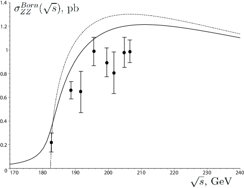
Figure 1: Born $ZZ$ cross-section in the Stable Particle Approximation (dashed line) and in the smeared-mass UP approach (solid line).

IV Calculation strategy and formalism

In this section we give the expressions for tree-level cross-sections and consider the strategy of radiative corrections (RC) accounting in the framework of the considering model. As it was shown in Refs. 32b ; 39 , the model description of UP is equivalent to some effective theory of UP, which includes the self-energy type RCs in all orders of perturbation theory. Moreover, the UP is the nonperturbative object in the vicinity of the resonance. So, the traditional program of RCs calculation is not valid in the framework of the model. We have no well defined set of the diagrams which is gauge invariant and renormalized. The model of UPs 32b is effective and not a gauge one, and we have no any rigid criteria for definition of such a set. So, we follow the strategy which is based on the simple phenomenology and was successfully applied earlier 34 ; 35 . For the preliminary analysis of the model applicability in description of the boson-pair production we restrict ourselves by taking into account of the major part of RCs which is common for all processes under consideration. This is so-called Initial State Radiation (ISR) correction which includes hard and soft real and virtual $\gamma$-radiation. It is needed for compensation of IR divergences.

We do not take into account any corrections to the final states of UPs because of the effective nature of these states in the framework of the model. We use the effective couplings $g(M_{Z})$ and $\alpha(M_{W})=1/127.9$ in the vertex with the final $Z,\,W,\,H$- and $\gamma$-states and $\alpha=1/137$ in the calculations of RCs. So, the principal part of the vertex corrections is effectively included into the coupling, and the low-energy behavior of the bremsstrahlung and radiative corrections to the initial states is taken into consideration.

The set of corrections, caused by the final state interactions in the $s$-channel diagrams is included into the effective coupling $\alpha(M_{W})$. The principal part of the so-called Coulomb singularity contributions, which were considered in Refs. 1 , 26a and 26bbb , can be also absorbed by the effective coupling. The one-loop calculation shows that this correction gives from $5.7\%$ at the threshold to 1.8% at 190 GeV 1 , while the total change of the effective coupling $\alpha(M_{W})$ with respect to $\alpha$ is about $7\%$. In the calculation we explicitly take into account the $O(\alpha)$ corrections including soft and hard bremsstrahlung, which are not described by the model and by the effective coupling. The real and virtual electromagnetic radiation should enter into the set of these RCs and mutually compensates the total IR divergences.

The program of RCs calculations, which is similar to above discussed one, was fulfilled in the series of papers (see, for example, Ref. 11 and references therein) for the case of the on-shell $W$-pair production (the limit of fixed masses $\mu_{1}=\mu_{2}=M^{2}_{W}$). The analytical expression for these corrections is represented in the compact and convenient form in Ref. 11 . We generalized this expression to the case of smeared-shell boson-pair production, that is for arbitrary values of mass parameters $\mu_{k}$, and applied it in our calculations. As a result, we get the cross-section $\sigma_{B_{1}B_{2}}(s;\mu_{1},\mu_{2})$ in the case of $B_{1}(\mu_{1})$ and $B_{2}(\mu_{2})$ production including above described corrections in the following form (see also Ref. 11 )

$$\sigma_{B_{1}B_{2}}(s;\mu_{1},\mu_{2})=\int_{0}^{k_{max}}\rho_{\gamma}(k)\sigma^{tr}_{B_{1}B_{2}}(s(1-k),\mu_{1},\mu_{2})\,dk\,,$$ (22)

where $\rho_{\gamma}(k)$ is the photon radiation spectrum 40 – 42 , $k=E_{\gamma}/E_{b}$ is the photon energy in units of beam energy and $s(1-k)$ is the effective $s$ available for the $B$-pair production after the photon has been emitted 11 . In the case of the on-shell $W$-pair production ($\mu_{1}=\mu_{2}=M^{2}_{W}$) the value $k_{max}=1-4M^{2}_{W}/s$ is the maximal part of the photon energy. The generalization of this value to the case $\mu_{1}\neq\mu_{2}$ leads to

$$k_{max}=1-2\frac{\mu_{1}+\mu_{2}}{s}+\frac{(\mu_{1}-\mu_{2})^{2}}{s^{2}}\equiv\lambda^{2}(\mu_{1},\mu_{2};s).$$ (23)

The photon distribution function is written in the form 11

$$\rho_{\gamma}(k)=\beta k^{\beta-1}(1+\delta^{v+s}_{1}+...)+\delta^{h}_{1}+...,$$ (24)

where we keep $O(\alpha)$ corrections only (i.e. $\delta_{n>1}=0$). The corresponding corrections are given ($v+s=$ virtual+soft, $h=$ hard) in Ref. 11 by

$$\beta=\frac{2\alpha}{\pi}(L-1),\,\,\,L=\ln\frac{s}{m^{2}_{e}},\,\,\,\alpha=\frac{1}{137};$$

$$\delta^{v+s}_{1}=\frac{\alpha}{\pi}(\frac{3}{2}L+\frac{\pi^{2}}{3}-2),\,\,\,\delta^{h}_{1}=\frac{\alpha}{\pi}(1-L)(2-k).$$ (25)

In analogy with Ref. 11 , we take into account an effective QCD correction factor in the multiplicative form $k_{QCD}=1+0.133/\pi$ 43 .

Now, we present the expressions for the cross-sections under consideration at the tree level. The scattering $e^{+}e^{-}\to ZZ$ is described by two standard $t$-channel diagrams. The model cross-section differs from the standard one due to various masses of $Z_{1}$ and $Z_{2}$ 34

$$\sigma^{st}(e^{+}e^{-}\rightarrow Z(m_{1})Z(m_{2}))=\frac{g^{4}(1+6c^{2}+c^{4})}{2^{10}\pi s\cos^{4}{\theta_{W}}}\bar{\lambda}(m_{1},m_{2};\sqrt{s})f(m_{1},m_{2};\sqrt{s}),$$ (26)

where $c=1-4\sin^{2}{\theta_{W}}$ and $g$ is the weak coupling constant. The functions $\bar{\lambda}(m_{1},m_{2};\sqrt{s})$ (normalized Källen function) and $f(m_{1},m_{2};\sqrt{s})$ are defined by the following expressions

$$\bar{\lambda}(m_{1},m_{2};\sqrt{s})=\left[1-2\,\frac{m^{2}_{1}+m^{2}_{2}}{s}+\frac{(m^{2}_{1}-m^{2}_{2})^{2}}{s^{2}}\right]^{1/2}$$ (27)

and

$$f(m_{1},m_{2};\sqrt{s})=-1+\frac{s^{2}+(m^{2}_{1}+m^{2}_{2})^{2}}{s(s-m^{2}_{1}-m^{2}_{2})\bar{\lambda}(m_{1},m_{2};\sqrt{s})}\arctan{\frac{s\bar{\lambda}(m_{1},m_{2};\sqrt{s})}{s-m^{2}_{1}-m^{2}_{2}}}.$$ (28)

The scattering $e^{+}e^{-}\to W^{+}W^{-}$ is described by one $t$-channel and two $s$-channel ($\gamma$, which is neglected, and $Z$ in the intermediate state) standard diagrams. The model cross-section at the tree level is as follows 35

$$\sigma^{tr}_{WW}(s;x_{1},x_{2})=\frac{\pi\alpha^{2}}{128s\sin^{4}\theta_{W}}F(s;x_{1},x_{2})\,,$$ (29)

where dimensionless function $F(s;x_{1},x_{2})$ is defined by the expression

$$F(s;x_{1},x_{2}) =\frac{16}{3(a^{2}-b^{2})(1-x_{Z})^{2}}\{3(a^{2}-b^{2})(a^{2}-b^{2}+2(1+a))(1-x_{Z})^{2}L(a,b)$$

$$+x_{Z}\cos(2\theta_{W})[3(b^{4}-2ab^{2}(2+a)+a^{3}(4+a))(1-x_{Z})L(a,b)$$

$$+2\lambda(a,b)(2b^{2}-3a^{2}-10a-1)(b^{2}(1-2x_{Z})-a(1-3x_{Z})-x_{Z})]$$

$$+\lambda(a,b)[x^{2}_{Z}\lambda^{2}(a,b)\cos(4\theta_{W})(2b^{2}-3a^{2}-10a-1)+12a^{3}z^{2}_{Z}$$

$$-a^{2}(3b^{2}(3x^{2}_{Z}-2x_{Z}+1)-49x^{2}_{Z}+30x_{Z}-15)-2a(b^{2}(19x^{2}_{Z}-10x_{Z}+5)$$

$$+8x^{2}_{Z})+2b^{4}(3x^{2}_{Z}-2x_{Z}+1)-2b^{2}(7x^{2}_{Z}-16x_{Z}+8)-2x^{2}_{Z}]\}.$$ (30)

In Eq. (IV) the dimensionless variables $a,b,x_{1},x_{2},x_{Z}$ and the functions $L(a,b)$ and $\lambda(a,b)$ are defined as follows

$$L(a,b)=\ln\biggl{[}\frac{1-a-\lambda(a,b)}{1-a+\lambda(a,b)}\biggr{]},\,\,\,\lambda(a,b)=\sqrt{1-2a+b^{2}},$$

$$x_{1,2}=\frac{m^{2}_{1,2}}{s},\,\,\,a=x_{1}+x_{2},\,\,\,b=x_{1}-x_{2},\,\,\,x_{Z}=\frac{M^{2}_{Z}}{s}.$$ (31)

The scattering $e^{+}e^{-}\to Z\gamma$ is described by two $t$-channel standard diagrams. The model cross-section at the tree level coincides with the standard one

$$\sigma^{tr}_{\gamma Z}(s,m_{Z})=\frac{\alpha g^{2}}{16\cos^{2}\theta_{W}s}\cdot\frac{1}{1-\mu_{Z}}\left[(1+c^{2}_{V})(1+\mu^{2}_{Z})[\ln(\frac{s}{m^{2}_{Z}}-1]+\frac{4m^{2}_{e}}{s}\right],$$ (32)

where $\mu_{Z}=m^{2}_{Z}/s$.

The scattering $e^{+}e^{-}\to ZH$, where $H$ is standard scalar Higgs boson, is described by one $s$-channel standard diagram with $ZZH$ vertex. This process is the most interesting one from the two points of view. Besides of its conceptual importance for the Standard Model verification, this process in the framework of the model has multiple factorisation structure. From the one hand, due to unstable $Z$ in the intermediate state, it is described by the universal factorized formula for the two-particle cross-section 38 . In the case under consideration, it has a simple factorized form

$$\sigma^{tr}(e^{+}e^{-}\to Z(s)\to ZH)=\frac{64\pi}{3(1-4m^{2}_{e}/s)}\frac{\Gamma^{ee}_{Z}(s)\Gamma^{ZH}_{Z}(s)}{(s-M^{2}_{Z})^{2}+s\Gamma^{2}_{Z}(s)}\,,$$ (33)

where $\Gamma^{ab}_{Z}(s)$ is the partial width of $Z$-boson, which has the mass $m^{2}=s$. Substitution of the expressions for the $\Gamma^{ee}_{Z}(s)$ and $\Gamma^{ZH}_{Z}(s)$ into Eq. (33) leads to the final expression for the cross-section in the limit of zero electron masses:

$$\sigma^{tr}_{ZH}(s;m_{Z},m_{H})=\frac{g^{4}M^{2}_{Z}}{108\pi\cos^{4}\theta_{W}}\frac{1-4\sin^{2}\theta_{W}+8\sin^{4}\theta_{W}}{(s-M^{2}_{Z})^{2}+s\Gamma^{2}_{Z}(s)}\bar{\lambda}(m^{2}_{Z},m^{2}_{H};s)\Big{[}1+\frac{(s+m^{2}_{Z}-m^{2}_{H})^{2}}{8sm^{2}_{Z}}\Big{]},$$ (34)

where $m_{Z}$ and $m_{H}$ are variable masses of $Z$-boson and Higgs boson. The value $\Gamma_{Z}(s)$ is defined in a standard way with the change $M^{2}_{Z}\to s$.

V Results

In this section we represent the results of the cross-section calculations in the smeared-shell UP model. In this approach we take into account the FWEs and the most important RCs (see the previous section). The model cross-section $\sigma(e^{+}e^{-}\to ZZ)$ including above mentioned corrections is represented in Fig. 2 (the solid line) together with result of the Monte-Carlo simulation (the dashed line) and LEP data points 44 . Both results are consistent with the data within the error bars and coincide with a very high precision. From this result it follows that the contribution of non-factorisable corrections in the considered energy range is negligibly small. So, one can apply our approach to the process $e^{+}e^{-}\to W^{+}W^{-}$ in this range. The lines start to differ slightly at energies larger than that of the available data, i.e. at $\sqrt{s}>200\,\mathrm{GeV}$. Note, however, that the difference between model and Monte-Carlo curves is an order of differences between results of various Monte-Carlo calculations.

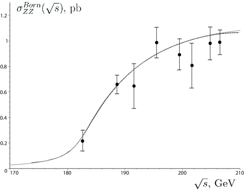
Figure 2: Total $ZZ$ cross-section obtained with the Monte-Carlo simulations (dashed line) and in the model of UP with smeared mass (solid line).

Now, we consider the corrected cross-section of the $W$-pair production.

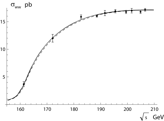
Figure 3: Model (dashed line) and Monte-Carlo RacconWW and YFSWW (solid lines) cross-sections of the process $e^{+}e^{-}\to W^{+}W^{-}$.

The model cross-section $\sigma_{WW}(s)$ was calculated numerically and represented in Fig. 3 as a function of $s$ by dashed line. The results of MC simulations, RacconWW 26c ; 26d and YFSWW 26e ; 26f , are represented for comparison by two barely distinguishable solid lines, and the experimental LEP II data 45 are given with the corresponding error bars. From Fig. 3, one can see that the model cross-section with RCs is in good agreement with the experimental data. Moreover, the deviation of the model from MC curves is significantly less then the experimental errors ($\lesssim 1\%$).

The cross-sections of the process $e^{+}e^{-}\to Z\gamma$ are given in Fig. 4 at the tree level for fixed ($M_{Z}$, short-dashed curve) and smeared boson mass (with an account of FWEs, dashed curve). The corrected cross-section (ISR, effective couplings, etc.) is represented in this figure by the solid curve. From the results of calculation it follows that the contribution of the FWEs and RCs is significant at threshold energy region $\sqrt{s}\gtrsim M_{Z}$. Unfortunately, we have no experimental data on the cross-section at this interesting energy range.

Figure 4: Born $Z\gamma$ cross-section in the Stable Particle Approximation (short-dashed line) and smeared mass approach (dashed line). Solid line represents the corrected cross-section.

The comparison of the model cross-section with the experimental data was fulfilled for exclusive process $e^{+}e^{-}\to\nu\bar{\nu}\gamma$ and $e^{+}e^{-}\to q\bar{q}\gamma$ at $160\lesssim\sqrt{s}\gtrsim 200\,\mbox{GeV}$. The model exclusive cross-section of the process with the final decays $Z\to f\bar{f}$ can be obtained by the changing $\rho(m)\to\rho(m)Br(Z(m)\to f\bar{f})$ in the formula (20). In Fig. 5 we represent the cross-section as a function of $\sqrt{s}$ within the UP model (solid curve) in comparison with the experimental data L3 applying the experimental cuts on the phase space.

Figure 5: Cross-section of the exclusive process $e^{+}e^{-}\to Z\gamma\to\nu\bar{\nu}\gamma$. Solid line represents corrected model cross-section.

One can see that the model description of the process under consideration is in good agreement with the experimental data. Some exceeding of the experimental points over the model curve at high-energy sector can be explained, for instance, by neglecting of the non-factorisable corrections.

Figure 6: Born $e^{+}e^{-}\to Z\to ZH$ cross-section in the Stable Particle Approximation (short-dashed line) and smeared mass approach (dashed line). Solid line represents the corrected cross-section.

Finally, we consider the cross-section of the process $e^{+}e^{-}\to Z\to ZH$ which is doubly factorisable within the UP model. In the Fig. 6 we represent the cross-section at the tree level in the case of fixed boson masses ($M_{Z}$ and $M_{H}=140$ GeV, short-dashed line) and the smeared masses (dashed line). The solid line represents the corrected model cross-section with an account of the above discussed RCs. From this figure, one can see the significant role of the threshold smearing at the threshold energy range. Analogously to previous case, RCs give quite noticeable contribution, especially in the peak region at $\sqrt{s}\sim 250-300$ GeV.

VI conclusion

The Finite Width Effects in the processes with participation of the unstable particles are usually described by the renormalized propagator, the decay-chain method, the convolution method and by the effective theory of unstable particles (UPs). In this paper, we applied the model of UPs with smeared mass for the description of the boson-pair production. The model describes the process $e^{+}e^{-}\to B_{1}B_{2}$ where bosons are on the smeared mass-shell. This approach is similar to the standard description of the off-shell $Z$- and $W$-pair production in the Semi-Analytical Approach. We have taken into account the soft and hard initial state radiation and a part of the virtual radiative corrections which are relevant in the framework of the model.

From our results it follows that the model is applicable to description of the near-threshold boson-pair production with LEP II accuracy. We get the total cross-section which is in good accordance with the experimental data; it coincides with the Monte Carlo calculations with a high precision. At the same time, the model provides a compact analytical expression for the cross-section in terms of convolution of the Born cross section with probability densities (or mass distributions) of bosons masses. However, we did not fulfill the detailed analysis of an accounting of the EW corrections, so this phenomenological formalism can not be directly applied for the precise description of the boson-pair production at high energies and for future experiments at ILC. From our results it follows, that the formalism under consideration can be convenient, simple and transparent framework for such a description. It is reasonable to consider the possibility of improvement of the approach and its applicability in the high precision calculations.

References

- (1) W. Beenakker et al., in Physics at LEP2, eds. G. Altarelli, T. Sjöstrand and F. Zwirner (CERN 96-01, Geneva, 1996), Vol. 1, p. 79; arXiv:hep-ph/9602351.
- (2) D. Bardin and G. Passarino, The Standard Model in the Making (Oxford University Press, 1999).
- (3) W Alles et al., Nucl. Phys. B 119, 125 (1977).
- (4) M. Lemoine and M. Veltman, Nucl. Phys. B 164, 445 (1980).
- (5) R. Philippe, Phys. Rev. D 26, 1588 (1982).
- (6) M. Bohm et al., Nucl. Phys. B 304, 463 (1988).
- (7) J. Fleischer et al., Z. Phys. C 42, 409 (1089).
- (8) W. Beenakker et al., Phys. Lett. B 258, 469 (1991).
- (9) W. Beenakker et al., Nucl. Phys. B 367, 287 (1991).
- (10) K. Kolodziej and M. Zralek, Phys. Rev. D 43, 3619 (1991).
- (11) J. Fleischer et al., Phys. Rev. D 47, 830 (1993).
- (12) W. J. Marciano and D. Wyler, Z. Phys. C 3, 181 (1979).
- (13) D. Albert et al., Nucl. Phys. B 166, 460 (1980).
- (14) K. Inoue et al., Prog. Theor. Phys. 64, 1008 (1980).
- (15) T. H. Chang et al., Nucl. Phys. B 202, 407 (1982).
- (16) F. Jegerlehner, Z. Phys. C 32, 425 (1986).
- (17) D. Yu. Bardin et al., Z. Phys. C 32, 121 (1986).
- (18) A. Denner and T. Sack, Z. Phys. C 46, 653 (1990).
- (19) T. Muta et al., Mod. Phys. Lett. A 1, 203 (1986).
- (20) G. Altarelli et al., in Physics at LEP2, CERN 96-01 (1996).
- (21) D. Y. Bardin et al., in Physics at LEP2, eds. G. Altarelli, T. Sjöstrand and F. Zwirner (CERN 96-01, Geneva, 1996), Vol. 2, p. 3; arXiv:hep-ph/9709270.
- (22) F. Boudjema et al., in Physics at LEP2, eds. G. Altarelli, T. Sjöstrand and F. Zwirner (CERN 96-01, Geneva, 1996), Vol. 1, p. 207; arXiv:hep-ph/9601224.
- (23) M. W. Grunewald and G. Passarino at al., CERN 2000-009 (2000); arXiv:hep-ph/0005309.
- (24) W. Beenakker et al., Nucl. Phys. B 548, 3 (1999).
- (25) A. Denner et al., Nucl. Phys. B 440, 95 (1995).
- (26) A. Denner et al., Nucl. Phys. B 519, 39 (1998).
- (27) A. Denner et al., Phys. Lett. B 612, 223 (2005); arXiv:hep-ph/0502063.
- (28) A. Denner et al., Nucl. Phys. B 724, 247 (2005); arXiv:hep-ph/0505042.
- (29) D. Bardin et al., arXiv:hep-ph/9602339.
- (30) S. Dittmaier et al., Nucl. Phys. B 376, 29 (1992).
- (31) M. L. Necrasov, arXiv:0709.3046.
- (32) A. Denner et al., Nucl. Phys. B 587, 67 (2000); arXiv:hep-ph/0006307.
- (33) A. Denner et al., Comput. Phys. Commun. 153, 462 (2003); arXiv:hep-ph/0209330.
- (34) S. Jadach et al., Phys. Rev. D 61, 113010 (2000).
- (35) S. Jadach et al., Comput. Phys. Commun. 140, 432 (2001).
- (36) A. Ballestrero et al., Comput. Phys. Commun. 152,175 (2003); arXiv:hep-ph/0210208.
- (37) M. Beneke et al., Phys. Rev. Lett. 93, 011602 (2004).
- (38) M. Beneke et al., Nucl. Phys. B 792, 89 (2008); arXiv:0707.0773 [hep-ph].
- (39) C. Schwinn, ECONFC0705302:LOOP 03 (2007); arXiv:0708.0730 [hep-ph].
- (40) M. L. Necrasov, arXiv:hep-ph/0002164.
- (41) P. T. Matthews and A. Salam, Phys. Rev. 112,283 (1958).
- (42) V. I. Kuksa, in Proceedings of the 17th Intl. Workshop on Quantum Field Theory and High Energy Physics, QFTHEP’03, Samara-Saratov, Russia, September 4-11, 2003, edited by M. Dubinin, V. Savrin (Skobeltsyn Institute of Nuclear Physics, Moscow State University), p. 350; arXiv:hep-ph/0612064].
- (43) V. I. Kuksa, Int. J. Mod. Phys. A 24, 1185 (2009).
- (44) I. F. Ginzburg, G. L. Kotkin, S. L. Panfil and V. G. Serbo, Nucl. Phys. B 228, 285 (1983) [Erratum-ibid. B 243, 550 (1984)].
- (45) L. Mandelstam and I. E. Tamm, J. Phys. (USSR) 9, 249 (1945).
- (46) P. Bush, arXiv:quant-ph/0105049.
- (47) A. D. Sukhanov, Phys. Part. Nucl. 32, 1177 (2001).
- (48) S. M. Bilenky et al., arXiv:0803.0527.
- (49) V. I. Kuksa, R. S. Pasechnik, Int. J. Mod. Phys. A 23, 4125 (2008).
- (50) V. I. Kuksa, R. S. Pasechnik, Int. J. Mod. Phys. A (in print) (2009); arXiv:0902.2857 [hep-ph].
- (51) O. Lalakulich, E. A. Paschos and M. Flanz, Phys. Rev. D 62, 053006 (2000).
- (52) V. I. Kuksa, Phys. Lett. B 633, 545 (2006).
- (53) V. I. Kuksa, Int. J. Mod. Phys. A 23, 4509 (2008).
- (54) V. I. Kuksa, Yad. Fiz. 72, 1108 (2009); arXiv:0902.4892 [hep-ph].
- (55) G. Bonneau and F. Martin, Nucl. Phys. B 27, 381 (1971).
- (56) M. Greco et al., Nucl. Phys. B 171, 118 (1980).
- (57) M. Bohm and W. Hollik, Nucl. Phys. B 204, 45 (1982).
- (58) F. Jegerlehner, in Testing the Standard Model (World Scientific, Singapore, 1991), p. 569.
- (59) DELPHI Collab. (J. Abdallah et al. Eur. Phys. J. C 30, 447 (2003); arXiv:hep-ex/0307050.
- (60) R. Strohmer, arXiv:hep-ex/0412019.
- (61) P. Achard et al. [L3 Collaboration], Phys. Lett. B 597, 119 (2004) [arXiv:hep-ex/0407012].