Large-scale collective motion of RFGC galaxies

Abstract

We processed the data about radial velocities and HI linewidths for $1678$ flat edge-on spirals from the Revised Flat Galaxy Catalogue. We obtained the parameters of the multipole components of large-scale velocity field of collective non-Hubble galaxy motion as well as the parameters of the generalized Tully-Fisher relationship in the “HI line width – linear diameter” version. All the calculations were performed independently in the framework of three models, where the multipole decomposition of the galaxy velocity field was limited to a dipole, quadrupole and octopole terms respectively. We showed that both the quadrupole and the octopole components are statistically significant.

On the basis of the compiled list of peculiar velocities of $1623$ galaxies we obtained the estimations of cosmological parameters $\Omega_{m}$ and $\sigma_{8}$. This estimation is obtained in both graphical form and as a constraint of the value $S_{8}=(\Omega_{m}/0.3)^{0.35}\sigma_{8}=0.91\pm 0.05$.

Keywords galaxies; large-scale structure; collective motion of galaxies; cosmological parameters

1 Introduction

The distribution of matter, including dark matter, in the Universe is inhomogeneous on the scales of about $100\,Mpc$. This is manifested, for example, in the existence of superclusters and voids. A galaxy, besides the cosmological expansion, is also attracted to the regions with greater density. As a result, the galaxies are involved in a non-Hubble large-scale collective motion on the background of Hubble expansion. In a more sophisticated way this can be considered as a development of initial density and velocity fluctuations in the early Universe due to the gravitational instability.

Investigation of such a motion is important at least for two reasons. First of all, it allows to plot the distribution of matter, including dark matter, in the surrounding region of the Universe, which is the main goal of cosmography, and to compare this distribution with the distribution of luminous matter. The second reason is that the parameters of this motion are linked with certain cosmological parameters, so we can obtain new independent estimations of these parameters. Of course, the accuracy of such estimation will not be very high, but the agreement of different estimations of cosmological parameters can support the correctness of the standard cosmological model.

In 1989 Karachentsev proposed to use flat edge-on spiral galaxies as a tool for studying their large-scale collective motion. They are good in this role for the following reasons:

1. The linear diameter is strongly correlated with the HI linewidth for thin bulgeless galaxies. This allows to determine distances without photometric data.

2. Flat galaxies can be easily identified by their axes ratio.

3. Flat galaxies have a nearly 100 per cent HI detection rate.

4. Galaxies in clusters are usually not flat due to interaction with neighbours. This means that flat galaxies avoid clustering and do not interact with the intergalactic gas in clusters.

5. Peculiar velocities of isolated flat galaxies are not perturbed by neighbours.

To implement this idea the Flat Galaxy Catalogue (FGC, Karachentsev et al., 1993) was created. It contained data about $N=4455$ galaxies, which satisfied the conditions $a_{b}/b_{b}\geq 7$ and $a_{b}>0.6^{\prime}$. Here $a_{b}$ and $b_{b}$ are the major and minor axial diameters directly measured on POSS-I and ESO/SERC plates. In accordance with the original photographic material, the Catalogue consists of two parts: FGC ($N=2573$) and its southern extension, FGCE ($N=1882$). The first part is based on the POSS-I and covers the sky region with declinations between $-20\deg$ and $+90\deg$. The second one is based on the ESO/SERC and covers the rest of the sky area up to $\delta=-90\deg$.

After thorough studies of the catalogue’s properties, both these parts were joined. The angular diameters from the FGCE were converted to the POSS-I system of the FGC, which appeared to be close to the $a_{25}$ system. This system, where galaxy size is taken at $B=25\,mag/\square^{\prime\prime}$ isophotal level, was used, in particular, by de Vaucouleurs et al. (1991). Some FGCE galaxies, which did not satisfy the condition $a>0.6^{\prime}$ after conversion, were removed from the resulting Revised Flat Galaxy Catalogue (RFGC, Karachentsev et al., 1999). It contained data about $N=4236$ galaxies including the information on the following parameters: Right Ascension and Declination for the epochs J2000.0 and B1950.0, galactic longitude and latitude, major and minor blue and red diameters in arcminutes in the POSS-I diameter system, morphological type of the spiral galaxies according to the Hubble classification, index of the mean surface brightness (I – high, IV – very low) and some other parameters, which are not used in this article. More detailed description of the catalogue can be found in the paper (Karachentsev et al., 1999).

The original goal of this catalogue was to estimate the distance to galaxies according to the Tully-Fisher relationship in the “HI line width – linear diameter” version without using their redshifts. The difference between the velocity $V$ derived from the redshift and the Hubble velocity $R=Hr$ corresponding to the distance $r$ estimated by Tully-Fisher relationship is called a peculiar velocity $V_{pec}=cz-Hr$. We can use such a simple form of the Hubble’s law because our sample has $z<0.1$.

There are some important things to take into account about peculiar velocities. The redshift includes not only the velocity of the galaxy, but also the velocities of our Galaxy, Solar System and the Earth. Thus, to eliminate these factors, all velocities were reduced to the frame, where CMB is isotropic. Naturally, the redshift gives us only the radial component of the velocity and the tangential components cannot be measured. Additionally, Tully-Fisher relationship is statistical and thus has a certain error. Thus, we can only estimate the peculiar velocity for each galaxy, sometimes with a significant error.

However, we believe that there is a large-scale velocity field. We consider the individual galaxies as test particles in the velocity field of large-scale collective motion. Thus, having data about the peculiar velocities of a large number of galaxies, we can restore the radial component of the velocity field. Using some additional assumptions, like the potentiality of the flux, it is possible to restore the 3D velocity field. For this reason we need ample samples of peculiar velocities, preferably uniformly covering the celestial sphere.

These conditions are satisfied by the RFGC catalogue, which covers the whole celestial sphere in both hemispheres with the natural exclusion of the Milky Way region. However, not all of the RFGC galaxies have data required to estimate the distance to them using the Tully-Fisher relationship. Nevertheless, the sample of galaxies having such data is also quite uniform, as shown on Fig. 1.

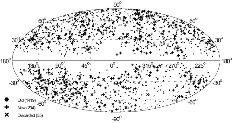
Fig. 1 : Distribution of galaxies over the celestial sphere in galactic coordinates

Naturally, RFGC is not the only sample that can be used for this purpose. Possible alternatives include SBF (Tonry et al., 1997, 2000), ENEAR (da Costa et al., 2000a), SFI (Haynes et al., 1999a, b), SFI++ (Springob et al., 2007), EFAR (Wegner et al., 1996; Colless et al., 2001), SMAC (Hudson et al., 1999, 2004), 2MFGC (Mitronova et al., 2003). However, in this article we use only the RFGC catalogue.

To apply the Tully-Fisher relationship the data from the catalogue is not sufficient; we also need to know the HI linewidth $W$ (in this article we take it at $50$ per cent level), or the gas rotation velocity $V_{rot}$ obtained from optical observations. Additionally, we need redshift data. The number of galaxies with such data increases constantly.

Since FGC and RFGC were assembled, a number of articles were published dealing with collective motions of RFGC galaxies. Very preliminary results were published by Karachentsev et al. (1995). The parameters of the bulk motion were calculated by Karachentsev et al. (2000b). In the paper
(Parnovsky et al., 2001) not only new data were added, but also the models featuring the quadrupole and octopole components of the velocity field were proposed. Also, the generalized Tully-Fisher relationship for RFGC galaxies was finalized. It included data not only about HI linewidth and angular diameter in red and blue bands, but also about the morphological type of the galaxy and its surface brightness index. By that time the authors had information about radial velocities and HI $21\,cm$ line widths or $V_{rot}$ for $1327$ RFGC galaxies from the different sources listed in the paper (Karachentsev et al., 2000b). From this number, $1271$ galaxies were included in the sample, and the rest of them were considered to be outliers. As a result, the first list of peculiar velocities of RFGC galaxies was prepared by Karachentsev et al. (2000a). Four years later, the number of galaxies with available data increased and reached $1561$ (Parnovsky & Tugay, 2004); $1493$ of them entered the sample. A new version of the list of peculiar velocities was prepared by Parnovsky & Tugay (2005). This list was the basis for solving the two abovementioned problems, namely mapping the matter density and estimation of cosmological parameters. The distribution of matter density was obtained in the paper (Sharov & Parnovsky, 2006) up to $75h^{-1}\,Mpc$ in the supergalactical plane and 8 more planes. In the same article, the excess masses of attractors in this region were estimated, and the estimation of $\beta$ parameter was obtained. The estimations of the cosmological parameters $\Omega_{m}$ and $\sigma_{8}$ were obtained in the paper (Parnovsky et al., 2006). The model was expanded taking into account the effects of general theory of relativity in the paper (Parnovsky & Gaydamaka, 2004).

An important result, obtained in the paper
(Parnovsky et al., 2001), and confirmed by
Parnovsky & Tugay (2004), was the statistical significance of quadrupole and octopole components (both at more than $99$ per cent confidence level). This result relied on the F-test, which assumes normal distribution of errors (see Hudson, 1964). However, even the normally distributed errors of angular diameters and HI linewidths and deviations from Tully-Fisher relationship lead to non-Gaussian distribution of peculiar velocities. Thus, the statistical significance of these terms required additional consideration. In the article (Parnovsky & Parnowski, 2008) it was shown using Monte-Carlo simulations that the statistical significance of these components appeared to be less than perceived from the F-test, but still large enough to be considered: the quadrupole was statistically significant at $96$ per cent confidence level and the octopole – at $90..93$ per cent confidence level.

In the four years that passed since the last list of peculiar velocities of RFGC galaxies was compiled, not only new data have appeared, but also some old data were remeasured. This led to a necessity of repeating all the steps required to obtain the new list. This means that not only new data have to be added, but the process of sample selection must be repeated from the very beginning. As it will be shown further, some results appeared to be notably different from the ones obtained with the previous sample.

In this paper we present the parameters of the large-scale collective velocity field in the framework of the multipole model as well as the estimations of some cosmological parameters. The distribution of matter density will be discussed in a separate article.

2 Multipole models of collective motion of galaxies

In the paper (Parnovsky et al., 2001) the velocity field components in the CMB reference frame were expanded in terms of galaxy’s radial vector $\vec{r}$. The first three terms are

$$V_{i}=D_{i}+A_{ik}r_{k}+O^{\prime}_{ikl}r_{k}r_{l}.$$ (1)

In our notation we use the Einstein rule: summation by all the repeating indices. Hence, for the radial velocity $V_{3K}$ in the CMB reference frame we get

$$V_{3K}=D_{i}n_{i}+rA_{ik}n_{i}n_{k}+r^{2}O^{\prime}_{ikl}n_{i}n_{k}n_{l},\,$$ (2)

where $\vec{n}=\vec{r}/r$ and $r=|\vec{r}|$. Let us decompose the tensor $\mathbf{A}$ in two parts: $A_{ik}=H\delta_{ik}+Q^{\prime}_{ik}$. Here $H$ is a trace, corresponding to the Hubble constant, $\delta_{ik}$ is the Kronecker delta, and $\mathbf{Q}^{\prime}$ is a traceless tensor. Next we switch from distance $r$ to the corresponding Hubble velocity $R=Hr$.

$$V_{3K}=R+D_{i}n_{i}+RQ_{ik}n_{i}n_{k}+R^{2}O_{ikl}n_{i}n_{k}n_{l},$$ (3)

where $\mathbf{Q}=H^{-1}\mathbf{Q}^{\prime}$ and $\mathbf{O}=H^{-2}\mathbf{O}^{\prime}$.

This decomposition was used to obtain some models of dependence of galaxy’s radial velocity $V$. In the simplest D-model (Hubble law + dipole) we have

$$V_{3K}=R+V^{dip}+\delta V,\,V^{dip}=D_{i}n_{i},$$ (4)

where $\vec{D}$ is a velocity of homogeneous bulk motion, $\delta V$ is a random deviation and $\vec{n}$ is a unit vector towards galaxy. After the addition of quadrupole terms we obtain a DQ-model

$$V_{3K}=R+V^{dip}+V^{qua}+\delta V,\,V^{qua}=RQ_{ik}n_{i}n_{k}$$ (5)

with symmetrical traceless tensor $\mathbf{Q}$ describing quadrupole components of the velocity field. It characterises the relative deviation of an effective “Hubble constant” in a given direction from the mean value. More detailed discussion will be given further. The DQO-model includes the octopole component of velocity field described by a symmetrical tensor $\mathbf{O}$ of rank 3:

$$\begin{array}[]{l}V_{3K}=R+V^{dip}+V^{qua}+V^{oct}+\delta V,\\ V^{oct}=R^{2}O_{ikl}n_{i}n_{k}n_{l}.\end{array}$$ (6)

In some cases it makes sense to use another way of describing the octopole component in the DQO-model. For this purpose the tensor $\mathbf{O}$ can be considered a sum of a traceless tensor $\mathbf{\hat{O}}$, and a trace, characterized by the vector $\vec{P}$

$$O_{ijk}=\hat{O}_{ijk}+P_{(i}\delta_{jk)},P_{i}=\frac{3}{5}O_{ijk}\delta_{jk}.$$ (7)

Here the indices in parantheses are symmetrized. Thus an alternative form of the DQO-model is

$$\begin{array}[]{l}V_{3K}=R+(D_{i}+R^{2}P_{i})n_{i}+RQ_{ik}n_{i}n_{k}\\ \phantom{V_{3K}=}{}+R^{2}\hat{O}_{ikl}n_{i}n_{k}n_{l}+\delta V.\end{array}$$ (8)

We will use Cartesian components of the vector $\vec{n}$ in the galactic coordinates:

$$\begin{array}[]{l}n_{1}=n_{z}=\sin b,n_{2}=n_{x}=\cos l\cos b,\\ n_{3}=n_{y}=\sin l\cos b.\end{array}$$ (9)

These three models were used for processing data on RFGC galaxies. To estimate the distances to galaxies a generalized Tully-Fisher relationship was used in the ‘linear diameter – HI line width’ version. It has a form (Parnovsky et al., 2001)

$$\begin{array}[]{l}R=(C_{1}+C_{2}B+C_{3}BT+C_{4}U)\frac{W}{a}\\ \phantom{R=}{}+C_{5}\left(\frac{W}{a}\right)^{2}+C_{6}\frac{1}{a},\end{array}$$ (10)

where $W$ is a corrected HI line width in $km\,s^{-1}$ measured at $50$ per cent of the maximum, $a$ is a corrected major galaxies’ angular diameter in arcminutes on red POSS and ESO/SERC reproductions, $U$ is a ratio of major galaxies’ angular diameters on red and blue reproductions, $T$ is a morphological type indicator ($T=I_{t}-5.35$, where $I_{t}$ is a Hubble type; $I_{t}=5$ corresponds to type Sc), and $B$ is a surface brightness indicator ($B=I_{SB}-2$, where $I_{SB}$ is a surface brightness index from RFGC; brightness decreases from I to IV). Details of corrections one can find in the papers (Parnovsky et al., 2001; Parnovsky & Tugay, 2004). The reasons for choosing this form of Tully-Fisher relationship for RFGC galaxies are given ibid. We only note that the statistical significance of each term in eq. (10) is greater than $99$ per cent.

Note that eq. (10) differs from the classical Tully-Fisher relationship, which has the form

$$R=C\frac{W^{\alpha}}{a}.$$ (11)

The corresponding analysis was performed in the paper (Parnovsky & Gaydamaka, 2004) for the relativistic model of motion. It was shown that the power $\alpha$ for the classical form of Tully-Fisher relationship (11) somewhat differs from 1. However, after including the corrections for the surface brightness and the morphological type of the galaxy, the value of $\alpha$ appeared to be close enough to 1 to use the form given by (10). If we repeat this analysis for the new data, the minimal variance is reached at $\alpha\sim 1.16$. At the same time the standard deviation $\sigma$ for the form (11) is $5..7$ per cent more than for the form (10) depending on the depth of the subsample and model used. If we combine the forms (10) and (11) into

$$\begin{array}[]{l}R=(C_{1}+C_{2}B+C_{3}BT+C_{4}U)\frac{W^{\alpha}}{a}\\ \phantom{R=}{}+C_{5}\left(\frac{W^{\alpha}}{a}\right)^{2}+C_{6}\frac{1}{a},\end{array}$$ (12)

we obtain the minimal variance at $\alpha\sim 1.05$, which is very close to 1. This correction does not reduce $\sigma$ due to the decreased number of degrees of freedom. This makes the introduction of $\alpha$ senseless. For this reason we will use only the form (10). This is additionally justified by the fact that all the coefficients enter this equation linearly and thus we can use the linear regression analysis.

The D-model has 9 parameters (6 coefficients $C$ and 3 components of vector $\vec{D}$), DQ-model has 14 parameters (5 components of tensor $\mathbf{Q}$ are added), and DQO-model is described by 24 coefficients. The values and errors of the coefficients were calculated by the least square method for different subsamples with distances limitation to make the sample more homogeneous in the depth (Parnovsky et al., 2001). We used the same weights for all datapoints. Since the quadrupole and octopole terms explicitly depend on $R$, an iteration procedure was used. Note that the coefficients of the generalised Tully-Fisher relationship and components of the velocity model were fitted simultaneously. The iterations converge rather quickly.

3 Description of data

Directly from the RFGC catalogue we take the angular diameters on blue and red reproductions, morphological type of a galaxy and its surface brightness index. The angular diameters are corrected for intrinsic absorption. From other sources we take the radial velocity in the CMB frame and the HI line width or the gas rotation velocity $V_{rot}$ obtained from optical observations. The line widths are corrected for cosmological expansion and for turbulence. The data on HI line widths for RFGC galaxies in the HyperLeda (Paturel et al., 2003a) catalogue are based on 149 sources, which have different reliability. The main sources used in previous versions of our samples are listed in the papers (Parnovsky et al., 2001; Parnovsky & Tugay, 2004; Karachentsev et al., 2000a, b; Parnovsky & Tugay, 2005). Since that time new large volumes of data on radial velocities and HI linewidths of galaxies were published (e.g., ref:Springob). For this reason we rechecked the original data on HI line widths of galaxies in previous samples and changed some of them. For each galaxy we used only the data of original measurements and did not average the data of different papers. In the cases when data from reliable sources differed significantly, we used less reliable sources to choose between them. We also checked the deviation of the distance to galaxy from the Tully-Fisher relationship in the D-model.

After revising data from the previous samples, we added new data measured during the last 5 years. We took HI linewidths from the original articles (Koribalski et al., 2004; Theureau et al., 2005; Doyle et al., 2005; Springob et al., 2005). In the case when $W$ was unavailable we converted $V_{rot}$ from the HyperLeda catalogue (Paturel et al., 2003b) to $W$ using the relationship $W=2.016*V_{rot}+20.6$, obtained by processing data for galaxies, which have both records. Note that there are rare cases of significant deviations from this relationship.

In the process of data preparation we constantly checked the deviations of the radial velocities from the velocities calculated in the D-model. Some data were obvious outliers. Such galaxies were rejected from the sample. As a result, we had all the necessary data for $1678$ galaxies, including $55$ outliers. Thus the sample contained $1623$ galaxies, including $204$ new and $1419$ old ones. It is noteworthy that some of the old data changed as well. The distribution of these galaxies over the celestial sphere is shown on Fig. 1. The mean radial velocity of old galaxies is $6000\,km\,s^{-1}$, and of new ones it is $5600\,km\,s^{-1}$. The mode in both cases is about $4800\,km\,s^{-1}$. The sample has $90\%$ completeness up to about $6000\,km\,s^{-1}$.

The farthest galaxies in the sample have radial velocities above $20000\,km\,s^{-1}$. However, at such scales the sample is inhomogeneous and incomplete. To deal with more homogeneous samples, we consider subsamples with distance limitation. They include all the galaxies satisfying the condition $R<R_{max}$ in the D-model and are used for all the three models. For this purpose we used the following iterative procedure. First, we calculate the distances to the galaxies using seed coefficients from the whole sample or another subsample with close $R_{max}$. Then we select the galaxies with $R<R_{max}$ and recalculate the coefficients using only their data, once again calculate the distances and so on. In most cases these iterations converge, but in some cases, more often for small $R_{max}$, we get a limit cycle. In this case we select only the galaxies whose distances are below $R_{max}$ for all sets of coefficients in this limit cycle.

We used different subsamples with $R_{max}$ ranging from $3000$ to $12000\,km\,s^{-1}$. In this paper we mostly present information for the subsamples with $R_{max}$ equal to $8000\,km\,s^{-1}$ ($r=80h^{-1}\,Mpc$) and $10000\,km\,s^{-1}$ ($r=100h^{-1}\,Mpc$).

4 Multipole structure of collective motion

The parameters of a generalized Tully-Fisher relationship for all three models and two $R_{max}$ values are given in Table 1 together with their statistical significance levels according to F-test. The $F$ values should be compared to $3.8$, $6.6$, $7.9$, $10.8$ and $12.1$, which correspond to $95$, $99$, $99.5$, $99.9$ and $99.95$ per cent confidence levels respectively. Most of them are statistically significant at $99.95$ per cent confidence level with the exception of $C_{3}$ for $R_{max}=10000\,km\,s^{-1}$. Comparing the coefficients to that of Parnovsky & Tugay (2004) one can see that $C_{1}$, $C_{4}$, $C_{5}$ and $C_{6}$ remain the same within the margin of error, and $C_{2}$ and especially $C_{3}$ are reduced, which means lesser influence of the morphological type of galaxies. This also leads to some decrease of statistical significance, which is still more than $95$ per cent.

Table 1 : Parameters of the generalized Tully-Fisher relationship (10)

$i$	D-model DQ-model DQO-model $C_{i}$ $F_{i}$ $c_{i}$ $F_{i}$ $c_{i}$ $F_{i}$

$R_{max}=8000$ km/s (1240 galaxies)
$1$	$15.8$ $\pm$	$1.6$	$103$	$17.2$ $\pm$	$1.6$	$122$	$17.4$ $\pm$	$1.6$	$126$
$2$	$1.84$ $\pm$	$0.20$	$80.5$	$1.96$ $\pm$	$0.21$	$90.0$	$1.95$ $\pm$	$0.21$	$88.4$
$3$	$-0.46$ $\pm$	$0.12$	$13.4$	$-0.49$ $\pm$	$0.13$	$15.2$	$-0.45$ $\pm$	$0.13$	$12.9$
$4$	$8.29$ $\pm$	$1.33$	$38.6$	$7.13$ $\pm$	$1.34$	$28.6$	$7.24$ $\pm$	$1.33$	$29.6$
$5$	$(-5.54$ $\pm$	$1.53)\times 10^{-3}$	$13.1$	$(-6.63$ $\pm$	$1.53)\times 10^{-3}$	$18.7$	$(-7.85$ $\pm$	$1.57)\times 10^{-3}$	$25.0$
$6$	$-825$ $\pm$	$86$	$92.4$	$-867$ $\pm$	$85$	$103$	$-883$ $\pm$	$85$	$107$
$R_{max}=10000$ km/s (1459 galaxies)
$1$	$16.3$ $\pm$	$1.4$	$143$	$17.3$ $\pm$	$1.4$	$157$	$17.2$ $\pm$	$1.4$	$156$
$2$	$1.38$ $\pm$	$0.18$	$59.3$	$1.44$ $\pm$	$0.18$	$62.1$	$1.55$ $\pm$	$0.18$	$70.6$
$3$	$-0.24$ $\pm$	$0.11$	$4.55$	$-0.26$ $\pm$	$0.11$	$5.32$	$-0.27$ $\pm$	$0.11$	$5.54$
$4$	$7.62$ $\pm$	$1.17$	$42.4$	$6.80$ $\pm$	$1.18$	$33.0$	$6.99$ $\pm$	$1.18$	$35.3$
$5$	$(-5.96$ $\pm$	$1.05)\times 10^{-3}$	$32.0$	$(-6.41$ $\pm$	$1.06)\times 10^{-3}$	$36.4$	$(-6.71$ $\pm$	$1.13)\times 10^{-3}$	$34.9$
$6$	$-785$ $\pm$	$87$	$81.8$	$-817$ $\pm$	$87$	$88.2$	$-845$ $\pm$	$87$	$94.9$

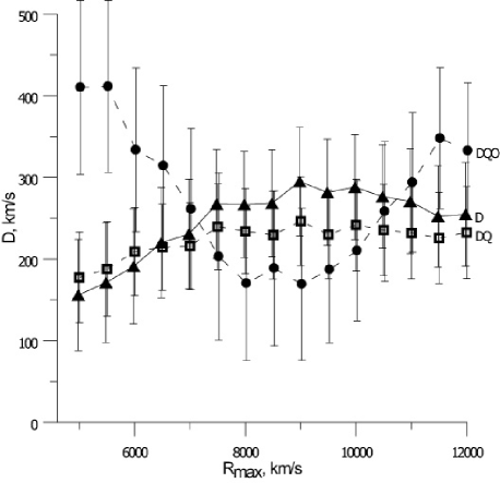
Fig. 2 : Dependence of the dipole component of the velocity on the sample depth for 3 models. Triangles correspond to the D-model, squares – to the DQ-model, and circles – to the DQO-model

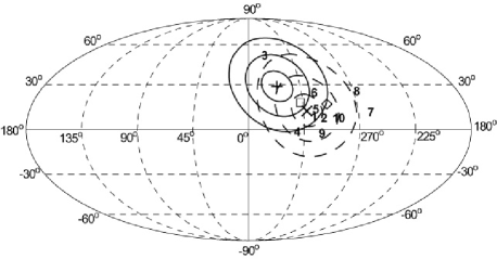
Fig. 3 : Bulk motion apices in galactic coordinates for $R_{max}=10000\,km\,s^{-1}$. Crosses mark the apices of the bulk motion in the D-model surrounded by $1\sigma$, $2\sigma$ and $3\sigma$ confidence areas. The square marks the apex position of the galaxies from the previous sample with corrected data. The diamond marks the apex position in the DQO-model. Solid boundaries correspond to new results, and dashed ones – to the results of Parnovsky & Tugay (2004). Numbers denote the results of other authors: 1 – (Lynden-Bell et al., 1988), 2 – (Hudson et al., 1995), 3 – (Lauer & Postman, 1994), 4 – (Parnovsky et al., 2001), 5 – (Dekel et al., 1999), 6 – (da Costa et al., 2000b), 7 – (Hudson et al., 2004), 8 – (Dale et al., 1999), 9 – (Kudrya et al., 2003), 10 – (Watkins et al., 2009)

The inclusion of the octopole component for subsamples with $R_{max}$ about $8000\,km\,s^{-1}$ leads to a drastic decrease of the dipole component up to $1\sigma$ level, as Parnovsky et al. (2001) have shown. This effect appeared to be even more evident in the paper (Parnovsky & Tugay, 2004). Such a strong dipole-octopole coupling can be explained by the same symmetry of these components with respect to the inversion of space. For the new sample this effect appeared to be weaker as the dipole component decreases only up to $2\sigma$ level (see Fig. 2). Naturally this effect is caused by incompleteness and asymmetry of the sample, which lead to dipole and octopole components being non-orthogonal.

This effect is important because D and DQO models yield the values of the bulk motion velocity differing by a factor of 2. Thus the dependence of the bulk motion velocity on the sample depth will be totally different for D and DQO models as one can see from Fig. 2. One should take this into account when analysing the convergence scale.

In comparison with the papers (Parnovsky et al., 2001) and (Parnovsky & Tugay, 2004), the apex direction of the dipole component has changed. In Table 2 we present its parameters for 2 subsamples together with the standard deviation $\sigma$ for D-model. Note that $\sigma$ includes both the intrinsic scatter in the generalised Tully-Fisher relationship and the stochastic component of the velocities, resulting in high values.

Table 2 : Parameters of the dipole component

Model	$R_{max}\hfil$ $D_{z}$ $D_{x}$ $D_{y}$ $D$ km/s	$l$, deg	$b$, deg	$\sigma$, km/s

D	$8000$	$147$ $\pm$	$47$	$176$ $\pm$	$58$	$-136$ $\pm$	$56$	$267$ $\pm$	$65$	$322$	$33$	$1045$
DQ	$8000$	$81$ $\pm$	$50$	$174$ $\pm$	$60$	$-134$ $\pm$	$58$	$234$ $\pm$	$52$	$323$	$20$	$1033$
DQO	$8000$	$-59$ $\pm$	$79$	$122$ $\pm$	$104$	$-103$ $\pm$	$100$	$170$ $\pm$	$95$	$320$	$-20$	$1020$
D	$10000$	$139$ $\pm$	$49$	$229$ $\pm$	$59$	$-106$ $\pm$	$59$	$288$ $\pm$	$64$	$335$	$29$	$1159$
DQ	$10000$	$70$ $\pm$	$53$	$200$ $\pm$	$62$	$-116$ $\pm$	$62$	$242$ $\pm$	$56$	$330$	$17$	$1151$
DQO	$10000$	$61$ $\pm$	$77$	$85$ $\pm$	$98$	$-182$ $\pm$	$97$	$210$ $\pm$	$86$	$295$	$17$	$1138$

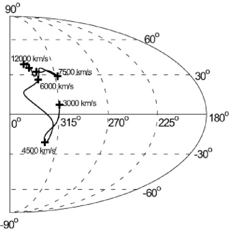
Fig. 4 : Dependence of bulk motion apex on the sample depth

The comparison of the results from Table 2 with those obtained earlier (Parnovsky et al., 2001; Parnovsky & Tugay, 2004) shows that the norm of the velocity hasn’t changed significantly, but the apex direction has. Let us discuss this question in detail. On Fig. 3 we present the Mollweide projection upon the celestial sphere of the ellipsoids corresponding to $1\sigma$, $2\sigma$ and $3\sigma$ confidence levels for the apex direction in the framework of D-model for $R_{max}=10000\,km\,s^{-1}$. Solid boundaries correspond to new results, and dashed ones – to the results of Parnovsky & Tugay (2004). One can see that the apex direction has changed at slightly more than $2\sigma$. Besides, on the Fig 3 we show the results of other authors: 1 – (Lynden-Bell et al., 1988), 2 – (Hudson et al., 1995), 3 – (Lauer & Postman, 1994), 4 – (Parnovsky et al., 2001), 5 – (Dekel et al., 1999), 6 – (da Costa et al., 2000b), 7 – (Hudson et al., 2004), 8 – (Dale et al., 1999), 9 – (Kudrya et al., 2003), 10 – (Watkins et al., 2009). One can see that the result of Parnovsky & Tugay (2004) matches other results better. The new result became closer to the result of Lauer & Postman (1994), but our norm is 2 times less. What caused such a deviation? We found the apex for ‘old’ galaxies used in previous samples but with corrected data for the HI linewidth. At this stage the apex has notably deviated from its original position. This position is shown on Fig. 3 by a square. After adding new data this deviation increased.

Let us discuss how much this deviation affects the global picture of the large-scale motion. Some authors believe that the norm and the apex of the dipole component are the most prominent characteristics of large-scale motion. This was true for very old samples with small depth. Our sample, however, has so large depth that it includes most nearest superclasters like the Great Attractor and Perseus-Pisces. For this reason, the first few components of the multipole decomposition (3) can not adequately describe all the radial velocity field of the large-scale motion. Moreso, this is hard to do with a single component (4). This phenomenon is due to the fact that a multipole decomposition is capable of describing very-large-scale motion with characteristic scale much larger than the scale of the sample, but can not describe the not-so-large-scale motions with characteristic scale less than the scale of the sample caused by attraction to these superclusters for any reasonable number of components.

Table 3 : Coefficients of the quadrupole component

$i$	$R_{max}=8000$ km/s $R_{max}=10000$ km/s DQ-model DQO-model DQ-model DQO-model $q_{i},\,\%$ $F_{i}$ $q_{i},\,\%$ $F_{i}$ $q_{i},\,\%$ $F_{i}$ $q_{i},\,\%$ $F_{i}$

1	$8.1$ $\pm$	$1.5$	$28.8$	$7.7$ $\pm$	$1.6$	$22.6$	$5.7$ $\pm$	$1.4$	$16.6$	$7.6$ $\pm$	$1.6$	$22.6$
2	$-2.1$ $\pm$	$1.6$	$1.6$	$-1.9$ $\pm$	$1.7$	$1.2$	$-1.9$ $\pm$	$1.5$	$1.7$	$-2.5$ $\pm$	$1.6$	$2.3$
3	$-0.8$ $\pm$	$2.2$	$0.1$	$-1.1$ $\pm$	$2.3$	$0.2$	$2.1$ $\pm$	$1.9$	$1.2$	$-1.2$ $\pm$	$2.1$	$0.3$
4	$0.9$ $\pm$	$2.3$	$0.1$	$1.2$ $\pm$	$2.5$	$0.2$	$4.1$ $\pm$	$2.1$	$4.0$	$2.6$ $\pm$	$2.5$	$1.1$
5	$1.7$ $\pm$	$2.7$	$0.4$	$0.1$ $\pm$	$2.8$	$0.0$	$1.7$ $\pm$	$2.5$	$0.5$	$-0.2$ $\pm$	$2.7$	$0.0$
Total			$6.44$			$5.10$			$4.63$			$4.85$

Table 4 : Eigenvalues and eigenvectors of the quadrupole tensor

$R_{max}$, km/s

$N$

Maximum Minimum Third axis $Q_{1},\,\%$ $l$ $b$ $Q_{2},\,\%$ $l$ $b$ $Q_{3},\,\%$ $l$ $b$

DQ-model
$3000$	$292$	$19.2$ $\pm$	$3.7$	$151$	$-7$	$-19.8$ $\pm$	$4.2$	$80$	$68$	$0.6$ $\pm$	$5.6$	$58$	$-20$
$6000$	$916$	$5.6$ $\pm$	$1.6$	$186$	$74$	$-8.5$ $\pm$	$1.8$	$59$	$10$	$2.9$ $\pm$	$2.4$	$327$	$13$
$7000$	$1068$	$7.3$ $\pm$	$1.5$	$198$	$81$	$-5.9$ $\pm$	$1.7$	$77$	$4$	$-1.3$ $\pm$	$2.3$	$347$	$7$
$8000$	$1240$	$8.1$ $\pm$	$1.4$	$142$	$87$	$-6.2$ $\pm$	$1.5$	$102$	$-2$	$-1.9$ $\pm$	$2.1$	$12$	$2$
$8500$	$1322$	$6.8$ $\pm$	$1.3$	$68$	$85$	$-5.2$ $\pm$	$1.5$	$106$	$-4$	$-1.6$ $\pm$	$2.0$	$16$	$-3$
$9000$	$1379$	$7.0$ $\pm$	$1.2$	$53$	$79$	$-5.6$ $\pm$	$1.4$	$109$	$-6$	$-1.4$ $\pm$	$1.8$	$18$	$-9$
$9500$	$1417$	$6.9$ $\pm$	$1.2$	$41$	$78$	$-5.4$ $\pm$	$1.4$	$109$	$-4$	$-1.5$ $\pm$	$1.8$	$18$	$-11$
$10000$	$1459$	$6.3$ $\pm$	$1.2$	$55$	$75$	$-4.4$ $\pm$	$1.3$	$105$	$-10$	$-1.9$ $\pm$	$1.8$	$13$	$-11$
DQO-model
$3000$	$292$	$22.3$ $\pm$	$4.3$	$153$	$-9$	$-19.9$ $\pm$	$4.3$	$80$	$63$	$-2.4$ $\pm$	$6.1$	$59$	$-26$
$6000$	$916$	$5.1$ $\pm$	$1.9$	$156$	$71$	$-7.8$ $\pm$	$1.9$	$56$	$3$	$2.8$ $\pm$	$2.7$	$325$	$19$
$7000$	$1068$	$6.6$ $\pm$	$1.8$	$124$	$81$	$-5.4$ $\pm$	$1.7$	$75$	$-6$	$-1.2$ $\pm$	$2.5$	$346$	$7$
$8000$	$1240$	$7.8$ $\pm$	$1.6$	$141$	$86$	$-5.9$ $\pm$	$1.6$	$90$	$-3$	$-1.9$ $\pm$	$2.3$	$360$	$3$
$8500$	$1322$	$7.5$ $\pm$	$1.6$	$133$	$84$	$-4.9$ $\pm$	$1.5$	$92$	$-5$	$-2.6$ $\pm$	$2.2$	$2$	$4$
$9000$	$1379$	$8.2$ $\pm$	$1.6$	$101$	$84$	$-5.1$ $\pm$	$1.5$	$90$	$-6$	$-3.1$ $\pm$	$2.2$	$359$	$1$
$9500$	$1417$	$7.8$ $\pm$	$1.6$	$93$	$86$	$-4.8$ $\pm$	$1.5$	$99$	$-4$	$-3.0$ $\pm$	$2.2$	$9$	$-1$
$10000$	$1459$	$7.8$ $\pm$	$1.6$	$120$	$83$	$-5.3$ $\pm$	$1.5$	$89$	$-6$	$-2.5$ $\pm$	$2.2$	$359$	$3$

As a result, the variation of the subsample depth $R_{max}$ can lead to significant deviation of the vector $\vec{D}$, especially when the supsample boundary crosses a large attractor. At smaller $R_{max}$ values we observe only the increase of radial velocity in the direction of the attractor. At larger $R_{max}$ we see also the backfall. In the framework of DQO-model these effects can be taken into account, but it is too much for the simple D-model to handle. On Fig. 4 we show the variation of the apex position in dependence from the sample depth. One can see that at small $R_{max}$ the apex crosses the galactic plane and approaches the results of most authors depicted on Fig. 3. An additional argument in favour of the apex deviation being not much of a problem is the following consideration. If in the framework of D-model with the same $R_{max}$ for each galaxy we introduce statistical weights corresponding to the variance of the radial velocity as a function of distance, the apex will correspond to the position $l=327\deg;\,b=18\deg$, which is closer to the result of Parnovsky & Tugay (2004). It is obvious that in such an approach the input from the nearest galaxies will dominate over the more distant galaxies.

Another possible explanation is that the velocity field is not well described by a pure dipole, and the dipole one recovers is unstable with respect to the limiting distance of the sample used. Furthermore, although the dipole is (in principle) a well-defined property of the field, and its mean convergence with distance is predictable within a given cosmological model, the problem here (as noted previously) is that the multipole basis is not orthogonal for this sample, so that in practice the dipole is not well-defined (in addition to varying stochastically with sample volume). As (Watkins et al., 2009) have shown, this sample bias in the measurement of the dipole is substantial, and has to be taken into account when comparing results from different samples.

As we mentioned before, the usage of the more complex DQO-model allows to describe such phenomena as the backfall. Besides, as it was shown by Parnovsky & Parnowski (2008), the mean deviation of the calculated apex from its true value, caused by measurement errors and the deviations from the Tully-Fisher relationship, is less in the DQO-model in comparison to the D-model. On Fig. 3 the relevant apex position for the DQO-model is denoted by a diamond. We can see that it fairly corresponds to the results of other authors.

As it was mentioned above, we used the generalised Tully-Fisher relationship in the form 10. However, we also calculated the bulk motion parameters in the D-model using the classical form 11. We obtained that the bulk motion velocity is $274\,km\,s^{-1}$ and the apex coordinates are $l=317$, $b=36$ for $R_{max}=10000\,km\,s^{-1}$. For $R_{max}=8000\,km\,s^{-1}$ the corresponding values are $254\,km\,s^{-1}$, $l=306$, $b=41$. As one can see from Table 2 and Fig. 3 these values fall in $1\sigma$ confidence areas.

Let us consider the quadrupole component. In Table 3 we present the corresponding coefficients. The traceless quadrupole tensor is described by 5 coefficients:

$$\begin{array}[]{l}V_{r}^{qua}=RQ_{ij}n_{i}n_{j}=R[q_{1}(n_{1}^{2}-n_{3}^{2})+q_{2}(n_{2}^{2}\\ \phantom{V_{r}^{qua}=}{}-n_{3}^{2})+q_{3}n_{1}n_{2}+q_{4}n_{1}n_{3}+q_{5}n_{2}n_{3}].\end{array}$$ (13)

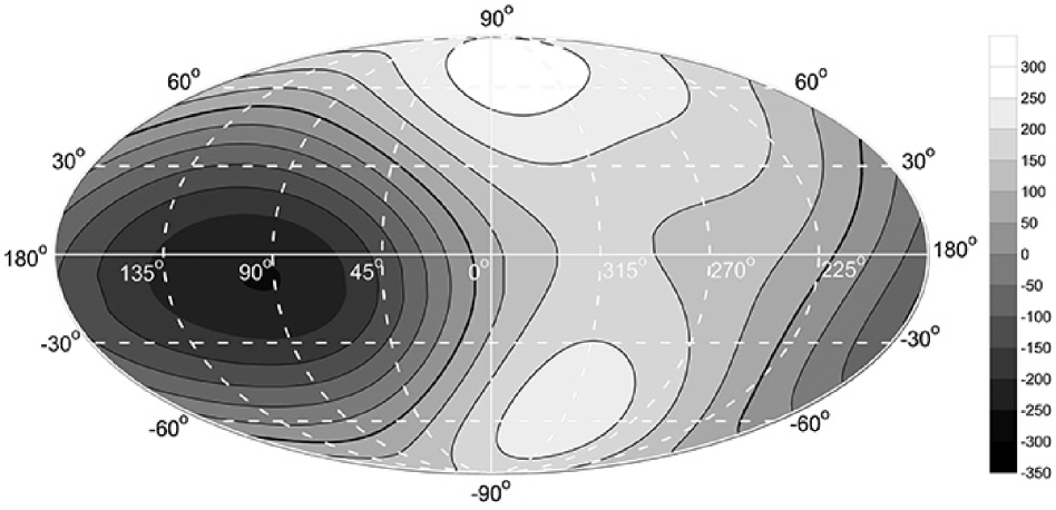
Fig. 5 : Distribution of radial velocity of collective non-Hubble motion at $20h^{-1}\,Mpc$

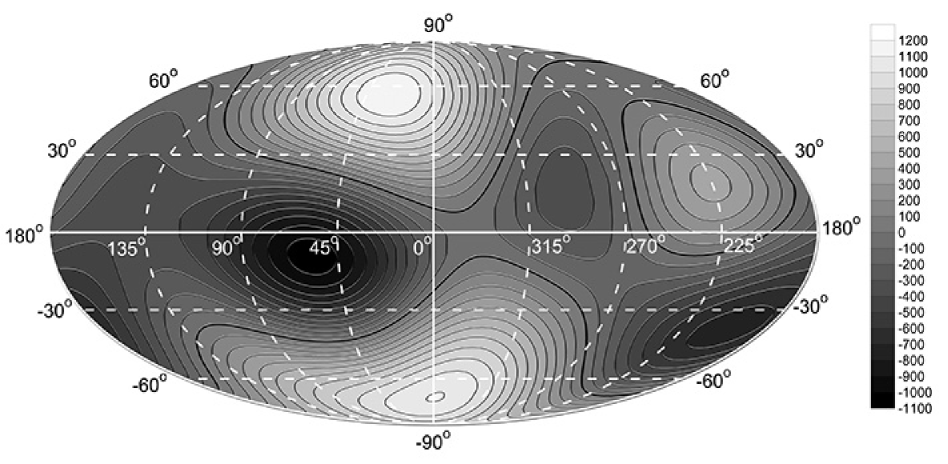
Fig. 6 : Distribution of radial velocity of collective non-Hubble motion at $80h^{-1}\,Mpc$

Table 5 : Coefficients of the octopole component

$i$	$R_{max}=8000$ km/s $R_{max}=10000$ km/s $d_{i}\cdot 10^{6}$ $F_{i}$ $d_{i}\cdot 10^{6}$ $F_{i}$

1	$7.2$ $\pm$	$3.9$	$3.5$	$-4.1$ $\pm$	$3.0$	$1.8$
2	$-2.1$ $\pm$	$5.2$	$0.2$	$-0.4$ $\pm$	$3.7$	$0.0$
3	$-3.7$ $\pm$	$5.4$	$0.5$	$-1.6$ $\pm$	$4.6$	$0.1$
4	$20.3$ $\pm$	$7.1$	$8.2$	$10.6$ $\pm$	$4.9$	$4.7$
5	$-7.8$ $\pm$	$7.4$	$1.1$	$4.3$ $\pm$	$6.1$	$0.5$
6	$24.0$ $\pm$	$7.6$	$9.8$	$23.0$ $\pm$	$5.5$	$17.5$
7	$-13.0$ $\pm$	$9.6$	$1.8$	$-12.5$ $\pm$	$8.0$	$2.4$
8	$10.9$ $\pm$	$7.8$	$2.0$	$15.8$ $\pm$	$6.1$	$6.8$
9	$-17.9$ $\pm$	$9.0$	$3.9$	$-6.2$ $\pm$	$6.9$	$0.8$
10	$33.8$ $\pm$	$10.2$	$11.1$	$25.9$ $\pm$	$7.6$	$11.7$
Total			$4.16$			$4.37$

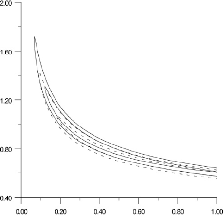
Fig. 7 : $1\sigma$ and $2\sigma$ confidence levels of cosmological constants $\Omega_{m}$ and $\sigma_{8}$ for the complex (solid) and simple (dashed) models

In Table 3 we also present the errors of these coefficients and their significances according to F-test. The quadrupole coefficients $q_{i}$ are close to the coefficients obtained by Parnovsky & Tugay (2004). One can see that the significance of all components except the first one is low. Nevertheless, the significance of the first component is high enough for the total significance of the whole quadrupole component to be sufficient. The $F$ values of the quadrupole component are the following: $4.63$ for the DQ-model and $R_{max}=10000\,km\,s^{-1}$, $4.85$ for the DQO-model and $R_{max}=10000\,km\,s^{-1}$, $6.44$ for the DQ-model and $R_{max}=8000\,km\,s^{-1}$, and $5.10$ for the DQO-model and $R_{max}=8000\,km\,s^{-1}$. This should be compared to $3.35$, which corresponds to the confidence level of $99.5$ per cent for 5 degrees of freedom. Thus the quadrupole component is statistically significant according to F-test at $99.5$ per cent confidence level both in DQ and DQO-models.

What is the physical sense of the quadrupole component? As one can see from the paper (Parnovsky et al., 2001), it can be naturally combined with the Hubble constant. As a result, we obtain the effective ‘Hubble constant’ depending on direction

$$H(l,b)=H(1+Q_{ik}n_{i}n_{k}).$$ (14)

Naturally, this effective ‘Hubble constant’ is caused by large-scale collective motion on the sample scale. To estimate the value of its anisotropy we found the eigenvalues and eigenvectors of tensor $Q$. The three eigenvectors are orthogonal and the sum of three eigenvalues is equal to zero because $\mathbf{Q}$ is a traceless tensor.

In Table 4 we present the maximum, minimum and medium eigenvalues and the corresponding eigenvectors for DQ and DQO-models and different $R_{max}$. To obtain the eigenvalues of this ‘Hubble constant’ we should add $100$ per cent to each of the listed values. For example, for the subsample with $R_{max}=10000\,km\,s^{-1}$ in the framework of DQ-model the maximal ‘Hubble constant’ is equal to $106.3$ per cent of the actual Hubble constant, and the minimal – $95.6$ per cent. We can see that the anisotropy is weak but statistically significant. The anisotropy is large only for very small scales less than $60h^{-1}\,Mpc$. As one can see from the Table 4, the maximum axis is dominant over the other two. However, the direction of the minimum axis is more stable for both DQ- and DQO-model. In the DQO-model the maximum axis is also stable at $R_{max}>6000\,km\,s^{-1}$. It lies almost in the supergalactic plane. The minimum direction deviates from this plane by approximately $30$ degrees of arc.

In the DQ-model the situation is different. As one can see from the Table 4, the variation of the maximum eigenvector is more evident. With the increase of $R_{max}$ the eigenvector starts deviating from the supergalactic plane and at $R_{max}=10000\,km\,s^{-1}$ this deviation reaches approximately $20$ degrees of arc. This effect can be explained by the fact that the Local Supercluster in this case constitutes the smaller fraction of the sample.

We also calculated the statistical significance of the octopole component in the DQO-model. The corresponding $F$ values are equal to $4.37$ for $R_{max}=10000\,km\,s^{-1}$ and $4.16$ for $R_{max}=8000\,km\,s^{-1}$. These values should be compared to the value $2.52$, which corresponds to the confidence level of $99.5$ per cent for $10$ degrees of freedom. Thus, the octopole component is also statistically significant according to F-test at $99.5$ per cent confidence level. The same qualitative conclusion was achieved in the paper (Parnovsky & Parnowski, 2008). We can also calculate the statistical significance of $\vec{P}$ in eq. (7) as in the paper (Parnovsky et al., 2001; Parnovsky & Tugay, 2004). Its $F$ values are equal to $0.21$ for $R_{max}=10000\,km\,s^{-1}$ and $2.50$ for $R_{max}=8000\,km\,s^{-1}$. This should be compared to $3.78$, $2.60$, $2.14$ and $0.79$, which correspond respectively to $99$, $95$, $90$ and $50$ per cent confidence levels for $3$ degrees of freedom. Thus, for $R_{max}=10000\,km\,s^{-1}$ the octopole trace is insignificant at $50$ per cent confidence level, and for $R_{max}=8000\,km\,s^{-1}$ it is significant at $90$ per cent confidence level, but this is insufficient to claim that this value is significant for all subsamples.

In Table 5 we present the coefficients of the octopole component, their errors and significances according to F-test. The octopole tensor including the trace $\vec{P}$ is described by $10$ coefficients:

$$\begin{array}[]{l}V_{r}^{oct}=R^{2}\hat{O}_{ijk}n_{i}n_{j}n_{k}=R^{2}(d_{1}n_{1}^{3}+d_{2}n_{2}^{3}\\ \phantom{V_{r}^{oct}=}{}+d_{3}n_{3}^{3}+d_{4}n_{1}n_{2}^{2}+d_{5}n_{1}n_{3}^{2}+d_{6}n_{2}n_{1}^{2}\\ \phantom{V_{r}^{oct}=}{}+d_{7}n_{2}n_{3}^{2}+d_{8}n_{3}n_{1}^{2}+d_{9}n_{3}n_{2}^{2}\\ \phantom{V_{r}^{oct}=}{}+d_{10}n_{1}n_{2}n_{3}).\end{array}$$ (15)

The coefficients of the octopole component differ from those given by Parnovsky & Tugay (2004) much stronger than the quadrupole ones. Nevertheless, their $1\sigma$ confidence areas overlap.

The knowledge of the coefficients of dipole, quadrupole and octopole components allows us to calculate the distribution of the radial velocity of the collective motion of galaxies. On Fig. 5 we present such a distribution for the DQO-model with $R_{max}=10000\,km\,s^{-1}$ and $R=2000\,km\,s^{-1}$, and on Fig. 6 – for $R_{max}=10000\,km\,s^{-1}$ and $R=8000\,km\,s^{-1}$. Note that the amplitudes of the dipole, quadrupole and octopole components are close to each other at $R\sim 6000\,km\,s^{-1}$. Thus, for larger distance like in Fig. 6 the octopole component prevails in the velocity field. This figure is characterised by a deep minimum of radial velocity in the direction opposite to the Great Attractor and Shapley concentration. In the direction to these superclusters there is also a minimum caused by a backfall to the Great Attractor. For smaller distances $R$ like in Fig. 5 this minimum becomes a maximum, but the minimum in the opposite direction is deeper than this maximum. It is clear that this picture is a simplified representation of the velocity field, but still it is much more complex than the simple bulk motion given by the D-model.

5 Estimation of some cosmological parameters and their combinations

As a result, we obtain not only the parameters of the multipole models of the collective motion, but also an estimation of the distance to galaxies using the generalised Tully-Fisher relationship. This allows us to compile a list of peculiar velocities for $1623$ galaxies. It can be used to estimate the cosmological parameters $\Omega_{m}$ and $\sigma_{8}$. For the previous version of the sample it was done in the paper (Parnovsky et al., 2006). We use a method similar to that used by Feldman et al. (2003) but with some changes. We calculate a 2-point correlation function for peculiar velocities, which is approximated by a formula obtained by Juszkiewicz et al. (1999). The formula has a nonlinear dependency on $\Omega_{m}$ and $\sigma_{8}$, thus these parameters can be estimated by the maximum likelihood method using the correlation function for RFGC galaxies. This yields an estimation of cosmological parameters $\Omega_{m}$ and $\sigma_{8}$ depicted on Fig. 7. There are 2 versions of the approximation formula: a simple one and a complex one. For the complex formula we obtain the values $\Omega_{m}=0.26$ and $\sigma_{8}=0.96$. This point is surrounded by $1\sigma$ and $2\sigma$ confidence areas. They have the banana-like shapes – very long and narrow curved strips. Judging from the boundaries of these areas, the errors of the cosmological parameters are very large. For this reason, the good agreement in the value of $\Omega_{m}$ between our estimation and other estimations can be just incidential. The simple model yields similar bananas.

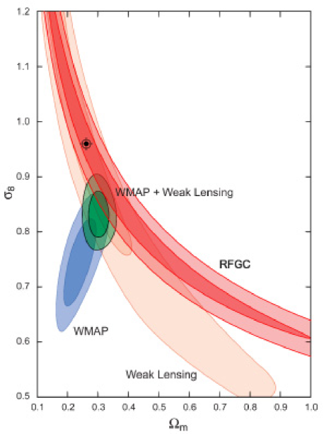
Fig. 8 : An estimation of cosmological constants $\Omega_{m}$ and $\sigma_{8}$ superimposed on 3-year WMAP results

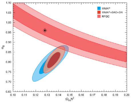
Fig. 9 : An estimation of cosmological constants $\Omega_{m}$ and $\sigma_{8}$ superimposed on 5-year WMAP results

Let us compare the obtained confidence areas with more accurate estimations. Let us start from the 3-year WMAP results. On Fig. 8 we reproduce Fig. 7 from the paper (Spergel et al., 2007) with an overlaid plot of $1\sigma$ and $2\sigma$ confidence areas for the complex model. The blue colour depicts WMAP data, the yellow colour depicts data obtained from weak gravitational lensing, the green colour depicts constraints imposed by both WMAP and lensing, and the red colour depicts our constraints. We can see that our results are similar to the weak lensing data much more than to WMAP data. In any case, these results are obtained with totally different methods, and their good correspondence is very promising.

The results of comparison with 5-year WMAP data are presented on Fig. 9. It is a reproduction of Fig. 19 from the paper (Komatsu et al., 2008) with an overlaid plot of $1\sigma$ and $2\sigma$ areas for the complex model. It contains constraints set by WMAP, mutual constraints set by WMAP, BAO and supernovae, and our constraints.

The main drawback of our estimation is its graphical form. In many cases it is preferable to deal with numerical constraints. To obtain such constraints we will make use of the long and narrow shape of our confidence areas. If we consider a combination of cosmological parameters of the form $(\Omega_{m}/0.3)^{\alpha}\sigma_{8}$ and $\alpha$ in the range from $0.3$ to $0.7$ we will obtain an estimation of the combination with better accuracy then either of the two cosmological parameters. The corresponding estimations are given on Fig. 10.

For the previous version of the sample the estimation of such a combination was made in the paper (Parnovsky, 2008). Ibid there are many estimations of other authors for different values of $\alpha$. Of all the values of $\alpha$ the smallest error was reached at $\alpha=0.35$. On Fig. 11 one can see the boundaries of $1\sigma$ confidence areas for the complex and simple models in the $(\Omega_{m}/0.3)^{0.35}\sigma_{8}$ against $\Omega_{m}$ coordinates. Both of them fit the constraint $(\Omega_{m}/0.3)^{0.35}\sigma_{8}=0.91\pm 0.05$. This result is almost the same as for the previous version of the sample ($0.93\pm 0.05$). The importance of this $\alpha$ value is caused by the fact that the value $S_{8}=(\Omega_{m}/0.3)^{0.35}\sigma_{8}$ was used in the paper (Evrard et al., 2008). As the author notes, the low estimation $S_{8}=0.69$ based upon WMAP and SDSS galaxies clusterisation leads to a number of problems. It leads to a contradiction with results of clusters formation modelling. The high estimation $S_{8}\sim 0.8-0.9$ lifts these problems. The estimation of the share of hot gas following from it corresponds to modern data obtained from the Sunyaev-Zel’dovich effect. Our results support the high estimation. Note that the paper (Evrard et al., 2008) contains many estimations obtained by different authors with different methods. Among them there are both high estimations, close to ours, and low estimations.

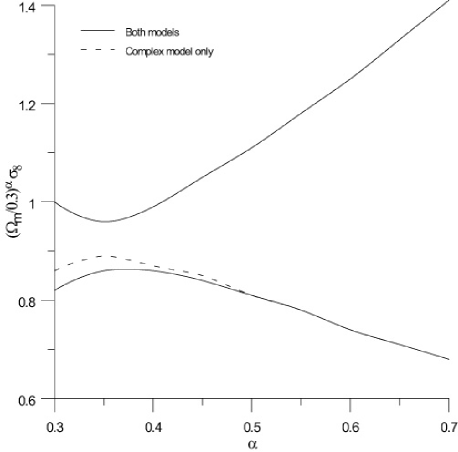
Fig. 10 : Dependence of $(\frac{\Omega_{m}}{0.3})^{\alpha}\sigma_{8}$ on $\alpha$. The solid line depicts constraint set by both models, the dashed line depicts constraint set only by the complex model only

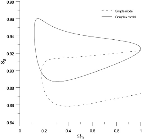
Fig. 11 : $1\sigma$ confidence areas of $S_{8}$ vs. $\Omega_{m}$ dependence. The solid line corresponds to the complex model, the dashed line corresponds to the simple model

6 Conclusion

We prepared a new increased and largely revised sample of RFGC galaxies with data about redshifts and HI linewidths. It allowed us to improve the estimations of parameters of the radial velocity field of large-scale collective motions of galaxies using 3 models of its multipole structure. In comparison with the previous versions the main features remained intact, but separate details, for example the apex of the dipole component of the bulk motion in the D-model, significantly changed. As before, the statistical significance according to F-test of both the quadrupole and the octopole components is well above $99.5$ per cent. The exact parameters are given in the article for subsamples with maximum distances $100h^{-1}\,Mpc$ and $80h^{-1}\,Mpc$.

The obtained velocity of the bulk motion is in agreement with the $\Lambda$CDM model expectation of $\sim 200\,km\,s^{-1}$. The value of the bulk motion velocity attracted additional attention after the recent paper of Watkins et al. (2009) who obtained this value as $407\pm 81\,km\,s^{-1}$ at the same scale $100h^{-1}\,Mpc$ as in present article. In this connection some authors immediately started speculating about the challenge to the $\Lambda$CDM model and the necessity for inclusion of non-gravitational forces (Ayaita et al., 2009).

For $1623$ galaxies we compiled a list of peculiar velocities which will be published in the nearest future. We also intend to use it to determine the distribution of the matter density (including dark matter) at the scales $75h^{-1}\,Mpc$ using POTENT method. This list was also used to estimate the cosmological parameters $\Omega_{m}$ and $\sigma_{8}$. The obtained constraint is given in graphical form on Fig. 7. The best numerical constraint is given by a combination $S_{8}=(\Omega_{m}/0.3)^{0.35}\sigma_{8}=0.91\pm 0.05$.

Acknowledgements

We acknowledge the usage of the HyperLeda database (http://leda.univ-lyon1.fr).

This research has made use of the NASA/IPAC Extragalactic Database (NED) which is operated by the Jet Propulsion Laboratory, California Institute of Technology, under contract with the National Aeronautics and Space Administration.

This article is published in the framework of Programme “Cosmomicrophysics” of the National Academy of Sciences of Ukraine.

References

- Ayaita et al. (2009) Ayaita, Y. et al., 2009 [arXiv:0908.2903]
- Colless et al. (2001) Colless, M. et al., 2001, MNRAS, 321, 277
- da Costa et al. (2000a) da Costa, L. N. et al., 2000a, Astron. J., 120, 95
- da Costa et al. (2000b) da Costa, L. N. et al., 2000b, ApJ, 537, L81
- Dale et al. (1999) Dale, D. A. et al., 1999, ApJ, 510, L11
- Dekel et al. (1999) Dekel, A. et al., 1999, ApJ, 522, 1
- Doyle et al. (2005) Doyle, M. T. et al., 2005, MNRAS, 361, 34
- Evrard et al. (2008) Evrard, A. E. et al., 2008, ApJ, 672, 122 (astro-ph/0702241)
- Feldman et al. (2003) Feldman, H. et al., 2003, ApJ, 596, L131 (astro-ph/0305078)
- Haynes et al. (1999a) Haynes, M. P. et al., 1999a, Astron. J., 117, 1668
- Haynes et al. (1999b) Haynes, M. P. et al., 1999b, Astron. J., 117, 2039
- Hudson (1964) Hudson, D. J., 1964, “Statistics Lectures on Elementary Statistics and Probability”, CERN: Geneva
- Hudson et al. (1995) Hudson, M. J. et al., 1995, MNRAS, 274, 305
- Hudson et al. (1999) Hudson, M. J. et al., 1999, ApJ, 512, L79
- Hudson et al. (2004) Hudson, M. J. et al., 2004, MNRAS, 352, 61
- Karachentsev (1989) Karachentsev, I. D., 1989, Astron. J., 97, 1566
- Karachentsev et al. (1993) Karachentsev, I. D. et al., 1993, Astron. Nachr., 314, 97
- Karachentsev et al. (1995) Karachentsev, I. D. et al., 1995, Astron. Nachr., 316, 369
- Karachentsev et al. (1999) Karachentsev, I. D. et al., 1999, Bull. SAO, 47, 5 (astro-ph/0305566)
- Karachentsev et al. (2000a) Karachentsev, I. D. et al., 2000a, Bull. SAO, 50, 5 (astro-ph/0107058)
- Karachentsev et al. (2000b) Karachentsev, I. D. et al., 2000b, Astron. Rep., 44, 150
- Komatsu et al. (2008) Komatsu, E. et al., 2008, ApJS, 180, 330 [arXiv:0803.0547]
- Koribalski et al. (2004) Koribalski, B. S. et al., 2004, Astron. J., 128, 16
- Kudrya et al. (2003) Kudrya, Yu. N. et al., 2003, A&A, 407, 889
- Juszkiewicz et al. (1999) Juszkiewicz, R. et al., 1999, ApJ, 518, L25
- Lauer & Postman (1994) Lauer, T. R. & Postman, M., 1994, ApJ, 425, 418
- Lynden-Bell et al. (1988) Lynden-Bell, D. et al., 1988, ApJ, 326, 19
- Mitronova et al. (2003) Mitronova, S. N. et al., 2003, Bull. SAO, 57, 5
- Parnovsky (2008) Parnovsky, S. L., 2008, Astron. Lett., 34, 451
- Parnovsky & Gaydamaka (2004) Parnovsky, S. L. & Gaydamaka, O. Z., 2004, Kinematics and Physics of Celestial Bodies, 20, 477
- Parnovsky & Tugay (2004) Parnovsky, S. L. & Tugay, A. V., 2004, Astron. Lett., 30, 357
- Parnovsky & Tugay (2005) Parnovsky, S. L. & Tugay, A. V., 2005, preprint (astro-ph/0510037)
- Parnovsky & Parnowski (2008) Parnovsky, S. L. & Parnowski, A. S., 2008, Astron. Nachr., 329, 864
- Parnovsky et al. (2001) Parnovsky, S. L. et al., 2001, Astron. Lett., 27, 765
- Parnovsky et al. (2006) Parnovsky, S. L. et al., 2006, Ap&SS, 302, 207
- Paturel et al. (2003a) Paturel, G. et al., 2003a, A&A, 412, 45
- Paturel et al. (2003b) Paturel, G. et al., 2003b, A&A, 412, 57
- Sharov & Parnovsky (2006) Sharov, P. Yu. & Parnovsky, S. L., 2006, Astron. Lett., 32, 287
- Spergel et al. (2007) Spergel, D. N. et al., 2007, ApJS, 170, 377 (astro-ph/0603449)
- Springob et al. (2005) Springob, C. M. et al., 2005, ApJS, 160, 149
- Springob et al. (2007) Springob, C. M. et al., 2007, ApJS, 172, 599 [arXiv:0705.0647]
- Theureau et al. (2005) Theureau, G. et al., 2005, A&A, 430, 373
- Tonry et al. (1997) Tonry, J. L. et al., 1997, ApJ, 475, 399
- Tonry et al. (2000) Tonry, J. L. et al., 2000, ApJ, 530, 625
- Tully & Fisher (1977) Tully, R. B. & Fisher, J. R., 1977, A&A, 54, 661
- de Vaucouleurs et al. (1991) de Vaucouleurs, G. et al., 1991, “Third Reference Catalogue of Bright Galaxies”, Springer: Berlin, Heidelberg, New York
- Watkins et al. (2009) Watkins, R. et al., 2009, MNRAS, 392, 743
- Wegner et al. (1996) Wegner, G. et al., 1996, ApJS, 106, 1