Partial CMB maps: bias removal and optimal binning of the angular power spectrum

Abstract

We present a semi-analytical method to investigate the systematic effects and statistical uncertainties of the calculated angular power spectrum when incomplete spherical maps are used. The computed power spectrum suffers in particular a loss of angular frequency resolution, which can be written as $\delta\ell\sim\pi/\gamma_{max}$, where $\gamma_{max}$ is the effective maximum extent of the partial spherical maps. We propose a correction algorithm to reduce systematic effects on the estimated $C_{\ell}$, as obtained from the partial map projection on the spherical harmonic $Y_{\ell}^{m}$ basis. We have derived near optimal bands and weighting functions in $\ell$-space for power spectrum calculation using small maps, and a correction algorithm for partially masked spherical maps that contain information on the angular correlations on all scales.

1 Introduction

The measurement of the temperature and polarisation anisotropies of the Cosmic Microwave Background (CMB) radiation provides essential information for testing the cosmological models and determining their parameters. Most of the statistical information present in the CMB temperature or polarisation sky maps can be encoded in the angular power spectrum $C_{\ell}$. An overview of the physical mechanisms responsible for the CMB anisotropies and the effect of the cosmological parameters on the power spectrum shape can be found in (Zaldarriaga et al, 1997) and (Hu & Dodelson, 2002).

The following references give an overview of some recent CMB power spectrum measurements: The all sky WMAP (Wilkinson Microwave Anisotropy Probe) space mission (Nolta et al (2009), Larson et al (2010)); ACBAR (Reichardt et al, 2009) which has made high resolution measurements using the Viper telescope at South Pole Station; the South Pole Telescope - SPT (Lueker et al, 2009); the Cosmic Background Imager-CBI (Mason et al, 2003) and the ACT telescope (Fowler et al, 2010) in the Atacama desert; the polarisation measurement at Amundsen-Scott South Pole Station by the Degree Angular Scale Interferometer - DASI (Carlstrom et al, 2003); as well as ballon borne experiments such as BOOMERANG (Jones et al (2006) , Masi et al (2006)), Archeops (Benoit et al (2003), Tristram et al (2005)) and MAXIMA (Lee et al, 2001). Table 1 summarizes typical sky coverage, the accessible $\ell$ range, and microwave frequency range for some of the above mentioned instruments.

Table 1: $\ell$-range and sky coverage for few of the microwave sky observation instruments

Name	sky cov. (deg2)	Angular Resolution (arcmin)	$\ell$ range (min-max)	frequency coverage (GHz)
WMAP	$\sim$ 40 000 (4 $\pi$ sr)	10-60	1-1500	23-94
ACBAR	600 (10 fields)	5	200-3000	150,220
BOOMERANG	750	6-10	10-1500	145,245,345
Archeops	5000	11 (@143)	10-700	143,217,353,545
CBI	40 (3 fields)	5-10	200-3500	26-36
SPT	100	$\sim$ 1	2000-9500	150,220
ACT	228	1.4	600-8000	148

Determining the CMB angular power spectrum is a complex process and the data analysis must take into account a number of effects, such as the non-stationnary noise contribution, non-circular instrumental beams, the sky scanning strategy and foreground contamination. A review of the general methods for CMB data processing can be found, for example, in (Tristram & Ganga, 2005).

The different systematic and statistical effects on CMB angular power specrtum estimates from partial sky maps have already been studied in length. In particular, several Montecarlo or analytical methods have been devised to evaluate or correct the impact of limited sky coverage on estimated angular power spectrum (Hivon et al (2002),Mitra et al (2009),Das et al (2009)).

In this paper we propose a different approach which is based on the analysis of the distortion of the angular correlation function. However, it should be noted that explicit computation of the angular correlation function is not needed. The use of the correlation function has also been studied by several authors, although with a different approach than the one developed here (Szapudi et al (2001a) , Szapudi et al (2001b)). In section 2, we recall briefly the main relations between the angular correlation function $\xi(\gamma)$ and the angular power spectrum $C_{\ell}$, and express them as a set of linear algebraic equations. Using this formalism in section 3, we compute the distortion of the estimated $C_{\ell}$ in incomplete sky maps and we show how the angular correlation function can be corrected to minimize these distortions. We show in particular that power spectrum estimates on partial maps suffer a loss of resolution in $\ell$-space and we propose near optimal $\ell$-space window function (binning).

The algebraic approach presented in section 3 can not be used to compute the variance of the reconstructed angular power spectrum (see paragraph 3.1 and 3.4). We have thus used Montecarlo simulations to estimate $C_{\ell}$ uncertainties. We present in section 4 the corresponding results for small maps ($\Omega\simeq 4\pi\times 10^{-2}$), representative of ground or balloon experiments such as OLIMPO (Nati et al, 2007), as well as the systematic shifts and possible correction for nearly complete maps ($\Omega\simeq 4\pi\times 0.9$) representative of space missions such as Planck (Planck Coll., 2006).

2 Angular correlation function and power spectrum from the full sphere

We recall here the basic relations for the angular power spectrum and correlation function. Detailed derivation of most of theses formulae can be found in (Magneville & Pansart, 2007) or (Wandelt et al, 2001).

We consider a real signal $s(\vec{\Omega})$ on the sphere ($S^{2}$), measured for each direction $\vec{\Omega}=(\theta,\phi)$. The function $s$ can be expanded on the spherical harmonic basis:

$$s(\theta,\phi) = \underset{l=0}{\overset{\infty}{\sum}}\underset{m=-\ell}{\overset{m=+\ell}{\sum}}a_{{\ell}{m}}\,Y_{\ell}^{m}(\theta,\phi)$$ (1)

$$a_{{\ell}{m}} = \int\limits_{S^{2}}s(\vec{\Omega})\,(Y_{\ell}^{m}(\vec{\Omega}))^{*}d\Omega$$ (2)

For an isotropic random signal, the angular power spectrum $C_{\ell}$ characterizes the statistical properties of the signal ($\langle\rangle$ denotes ensemble average).

$$\langle a_{{\ell}{m}}a_{{\ell^{\prime}}{m^{\prime}}}^{*}\rangle = \delta_{\ell-\ell^{\prime}}\delta_{m-m^{\prime}}C_{\ell}$$ (3)

It is possible to compute an unbiased power spectrum estimator $\widehat{C}_{\ell}$ from the spherical harmonic expansion coefficients. The $\widehat{C}_{\ell}$ coefficients are independent random variables with variance $\sigma^{2}_{\widehat{C}_{\ell}}$ (cosmic variance):

$$\widehat{C}_{\ell} = \frac{1}{2\ell+1}\underset{m=-\ell}{\overset{m=+\ell}{\sum}}\mid{a_{{\ell}{m}}}\mid^{2}$$ (4)

$$\langle\widehat{C}_{\ell}\rangle = C_{\ell}$$

$$\sigma^{2}_{\widehat{C}_{\ell}} = \frac{2}{2\ell+1}C_{\ell}^{2}$$ (5)

For an isotropic signal, the angular correlation function $\xi(\gamma)$ can also be used to characterize the signal properties, where $\gamma$ is the separation angle ($\cos\gamma=\vec{\Omega}\cdot\vec{\Omega^{\prime}}$) :

$$\xi(\gamma) = \frac{1}{4\pi}\underset{l=0}{\overset{\infty}{\sum}}(2\ell+1)C_{\ell}P_{\ell}(\cos\gamma)$$ (6)

$$C_{l} = 2\pi\;\int\limits_{-1}^{+1}\;\xi(\gamma)\;P_{l}(\cos\gamma)\;d\cos\gamma$$ (7)

It should be noted that the above relation holds also for the computed angular correlation function ($\hat{\xi}(\gamma)$) and power spectrum ($\widehat{C}_{\ell}$) for a given sky realization.

$$\hat{\xi}(\gamma) = \frac{1}{4\pi}\underset{l=0}{\overset{\infty}{\sum}}(2\ell+1)\widehat{C}_{\ell}P_{\ell}(\cos\gamma)$$

$$= \frac{1}{\mathcal{N}(\gamma)}\int\limits_{S^{2}\times S^{2}}s(\vec{\Omega})\,s(\vec{\Omega^{\prime}})\delta\left(\cos\gamma-\vec{\Omega}.\vec{\Omega^{\prime}}\right)d\Omega d\Omega^{\prime}$$

$$\mathcal{N}(\gamma) = \int\limits_{S^{2}\times S^{2}}\delta\left(\cos\gamma-\vec{\Omega}.\vec{\Omega^{\prime}}\right)d\Omega d\Omega^{\prime}=8\pi^{2}$$

The above relations, analogous to Fourier series, contain algebraic (sum) and analytic (integral) expressions, and involve the discrete variable $\ell\in\mathbb{N}$, as well as the continuous variable $\gamma\in[0,\pi]$. We can rewrite these expressions in a purely algebraic form, similar to the Discrete Fourier Transform (DFT). Indeed, if the $C_{l}$ spectrum is negligible for large $\ell>\ell_{max}\;$, and for any set of discrete values $\{\gamma_{i}\}$ of the $\gamma$ angle, the relations 6 and 2 can be written in matrix form:

$$\left[\xi(\gamma_{i})\right]\;=\;\left[\xi_{i}\right]=\left[\left[\mathbf{K_{i\ell}}\right]\right]*\left[C_{\ell}\right]$$ (9)

In the particular case where the number of $\gamma_{i}$ values is equal to the $\ell_{max}+1$ non-zero $C_{\ell}$ values, the $\left[\left[\mathbf{K_{i\ell}}\right]\right]$ matrix would be square. It can then be shown that the separation angles $\gamma_{i}$ at which the correlation function $\xi$ is computed ($\xi_{i}=\xi(\gamma_{i})$), could be choosen such that the square matrix $\left[\left[\mathbf{K}\right]\right]$ of size $(\ell_{max}+1)\times(\ell_{max}+1)$ is non-singular (see appendix). The equation (9) may thus be inverted to get:

$$\left[C_{l}\right]\;=\;\left[\left[\mathbf{K}\right]\right]^{-1}*\left[\xi_{i}\right]$$ (10)

Moreover, these $\gamma_{i}$ values are not very different from $\ell_{max}+1$ equidistant $\gamma$, distributed from $0$ to $\pi$, with the matrix elements close to $\left[\left[\mathbf{K}\right]\right]^{-1}_{\ell,i}\propto P_{\ell}(\cos\gamma_{i})$.

3 Angular power spectrum from partial maps

3.1 Angular correlation function distortion

The above equation (10) can be used to analyse the impact of any linear distortion of $\xi$ on the calculated $C_{l}$. Any linear distortion of the angular correlation function (including truncation for $\gamma>\gamma_{max}$) can be represented by a matrix $\mathbf{[[D]]}$ applied to $\xi$.

$$\langle\left[\xi(\gamma)\right]^{d}\rangle = \left[\left[\mathbf{D}\right]\right]*\left[\xi(\gamma)\right]$$

$$\langle\left[C_{l}\right]^{d}\rangle = \left[\left[\mathbf{K}\right]\right]^{-1}*\left[\left[\mathbf{D}\right]\right]*\left[\left[\mathbf{K}\right]\right]*\left[C_{l}\right]$$

$$\langle\left[C_{l}\right]^{d}\rangle = \left[\left[\mathbf{B_{c}}\right]\right]*\left[C_{l}\right]$$

$$\left[\left[\mathbf{B_{c}}\right]\right] = \left[\left[\mathbf{K}\right]\right]^{-1}*\left[\left[\mathbf{D}\right]\right]*\left[\left[\mathbf{K}\right]\right]$$ (11)

It should be stressed that in most cases, we can only compute the mean distortion caused by the measurement process, in particular due to the incomplete coverage. The above relations will not hold in general for a given realization or a single measurement. It will only be valid when an ensemble average is taken for the angular correlation function and power spectrum. This explains why it can not be used to estimate statistical uncertainties on the computed power spectrum.

Using the formalism described above, we have computed the effect of distorting or modifying the angular correlation function in some typical cases such as:

• Application of a sharp or a smooth cut $\xi(\gamma)\rightarrow\xi^{d}(\gamma)=\xi(\gamma)*\mathrm{Cut}(\gamma)$ to the angular correlation function. In the case of a sharp cut, $\xi(\gamma)$ is set to zero for $\gamma>\gamma_{max}$ (step function cut).

• Undersampling $\xi_{i}$ by a factor $p>1$, i.e. $\xi_{i}$ known only for $i=k\times p$

• Binning effect, where $\xi(\gamma_{i})$ is replaced by the mean value of $\xi$ in a small interval around $\gamma_{i}$. The binning can represent the distortion of the $\xi$ when computed through the histogram of all pixel pair products $s(\vec{\Omega})s(\vec{\Omega^{\prime}})$, binned as a function of their separation angle $\gamma$ ($\vec{\Omega}\cdot\vec{\Omega^{\prime}}=\cos(\gamma)$).

Figure 1 illustrates the effect of restricting the $\gamma$ range to $\gamma_{max}=30^{\circ}$ (i.e. setting $\xi(\gamma)=0$ for $\gamma>\gamma_{max}$), (left) and the undersampling (right). Restricting the range of angles for $\xi(\gamma)$, creates a correlation between different $\ell$ while undersampling produces an aliasing effect. Both of these effects are analogous to well known effects in standard Fourier analysis.

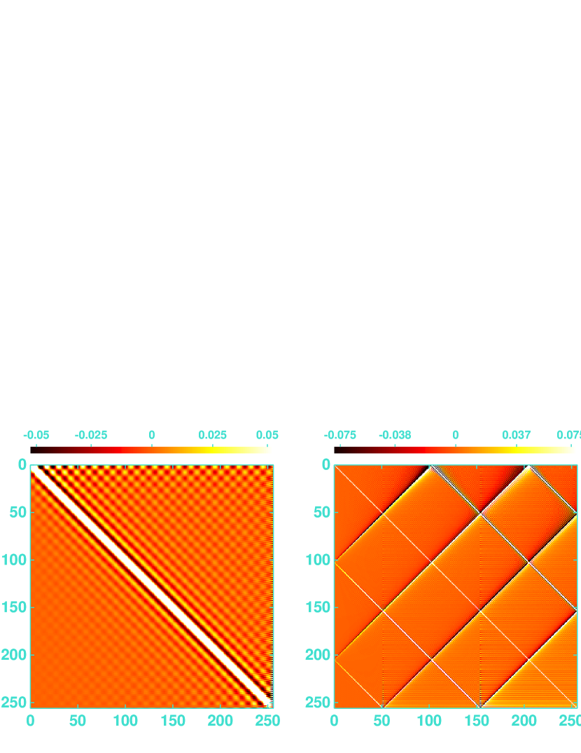
Figure 1: Color scale representation of the $\left[\left[\mathbf{B_{c}}\right]\right]$ matrix relating $\langle\widehat{C}_{\ell}^{t}\rangle\leftrightarrow C_{\ell}$. Left: Correlation effect induced by restricting the angular range to $\gamma<30^{\circ}$. Right: aliasing effect when $\xi$ is undersampled by factor p=5. The color scale has been chosen to enhance visually the matrix structure (the diagonal terms are around $\sim 0.15-0.2$).

3.2 Partial maps : truncated $\xi^{t}(\gamma)$

When the angular correlation function is calculated from maps with a maximal extent $\gamma_{max}$, nothing can be known on the correlation function for $\gamma>\gamma_{max}$. In addition, the statistical errors on the estimated correlation function will be larger compared to the one computed on the corresponding full ($4\pi$) map. It is well known that computing the angular power spectrum from a truncated $\xi^{t}(\gamma)$ using the integral equation (7) or the linear combination equation (10) produces spurious oscillations. However, these oscillations can be filtered out if the resulting power spectrum is binned.

$$\langle\widehat{C}_{\ell}^{t}\rangle = \left[\left[\mathbf{B_{c}}\right]\right]*\left[C_{\ell}\right]$$ (12)

$$\widehat{C}_{L}^{t} = \sum_{\ell}w_{L}(\ell)\widehat{C}_{\ell}^{t}$$ (13)

The filtered or weighted power spectrum $\widehat{C}_{L}^{t}$ defined here is obtained by applying the weight function $w_{L}(\ell)$ to the power spectrum $\widehat{C}_{\ell}^{t}$. The weight function should be centered around $L$ and normalised such that $\underset{l}{\overset{}{\sum}}\;w_{L}(\ell)\;=\;1$. The $w_{L}(\ell)$ would be in general positive, with a maximum for $\ell=L$ and decreasing to zero ( $w_{L}(l)\rightarrow 0$) when $\mid{\ell-L}\mid$ increases. The expectation value of the filtered spectrum can then be expressed using the weight matrix $\left[\left[\mathbf{W}\right]\right]_{L,\ell}=w_{L}(\ell)$:

$$\langle\widehat{C}_{L}^{t}\rangle = \left[\left[\mathbf{W}\right]\right]*\left[\left[\mathbf{B_{c}}\right]\right]*\left[C_{\ell}\right]$$ (14)

$$\langle\widehat{C}_{L}^{t}\rangle = \left[\left[\mathbf{B_{cW}}\right]\right]*\left[C_{\ell}\right]$$ (15)

We have computed the matrix $\left[\left[\mathbf{B_{cW}}\right]\right]$ relating true expectation values of $C_{\ell}$ to mean value of the weighted power spectrum $\langle\widehat{C}_{L}^{t}\rangle$ from truncated angular auto-correlation function. The results shown here correspond to $\xi(\gamma)$ truncated above $\gamma_{max}=30^{\circ}$, for Gaussian or square (step-wise) weight functions. Figure 2 shows one of the rows of the $\left[\left[\mathbf{B_{cW}}\right]\right]$ matrix around $\ell\sim 500$ for different weight functions. For Gaussian weights width $\sigma_{\ell}\gtrsim\dfrac{\pi}{\gamma_{max}}$, the effective $\ell$-space window or filter function becomes numerically very close to the corresponding Gaussian function. It can be seen also that applying top hat or square weights result in an effective window function significantly different from the corresponding square function. We have checked that this property and the value of optimal weight function width $\sigma_{\ell}\simeq\dfrac{\pi}{\gamma_{max}}$ does not depend on the value of the central $L$, at least for large enough $L\gtrsim\sigma_{\ell}$.

Our computation and simulations suggest that a Gaussian function with a width $\Delta\ell\sim\sigma_{\ell}=\dfrac{\pi}{\gamma_{max}}$ is a near optimal binning when the angular power spectrum is calculated from partial maps with maximum angular extent $\sim\gamma_{max}$. The word “optimal” should be understood in its common sense, and not the mathematical one, as the optimal solution depends on the chosen quantitative criteria. For example, different binning should be used if one seeks to increase the spectral resolution or if one is concerned by the statistical errors. As explained above, the suggested Gaussian binning has the following properties:

• The Gaussian weighted corrected angular spectra reduces the window function tails by an order of magnitude, compared to pseudo-$C_{\ell}$, while maintaining the $\ell$-space resolution as well as similar statistical uncertainties (see section 4). Using top hat (square) binning yields a window function with long tails and oscillations.

• The resulting true $\ell$-space window function is nearly identical to the weight or filter function applied to the computed $C_{\ell}$, with a simple analytical expression (Gaussian). This property is useful for presenting measured power spectra.

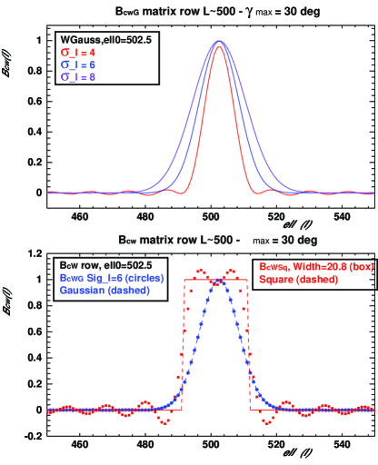
Figure 2: Weighted $\widehat{C}_{L}^{t}$ calculation truncated $\xi$ at $\gamma_{max}=30^{\circ}$. Top: Row of the weighted Bct matrix ($\left[\left[\mathbf{B_{cW}}\right]\right]$) around $L\sim 500$ for Gaussian weights ($B_{cWG}$) with three different widths $\sigma_{\ell}=4,6,8$. Bottom: Comparison of $B_{cW}$ matrix row for $L\sim 500$ with the corresponding Gaussian weights ($\sigma_{\ell}=6$), in blue and top hat (square) weighted ($B_{cWSq},\mathrm{width}=6\times\sqrt{12}=20.8$) in red.

When the power spectrum is estimated using incomplete spherical maps, a loss of resolution in angular frequencies ($\Delta\ell\sim\pi/\gamma_{max}$) can also be understood using linear combinations of Legendre polynomial. We define new functions $Q_{L}$, through linear combinations of Legendre polynomials around a given $L$, with Gaussian weights :

$$\begin{array}[]{lcl}Q_{L}^{\sigma_{l}}&=&\frac{1}{\Sigma w}\sum_{l}\exp\left[\frac{(\ell-L)^{2}}{2\sigma_{\ell}^{2}}\right]\,P_{\ell}\\ \Sigma w&=&\sum_{l}\exp\left[\frac{(\ell-L)^{2}}{2\sigma_{\ell}^{2}}\right]\\ Q_{L}^{\sigma_{l}}(\cos\gamma)&\simeq&P_{\ell}(\cos\gamma)\hskip 14.22636pt\gamma<\pi/\sigma_{\ell}\\ Q_{L}^{\sigma_{\ell}}(\cos\gamma)&\simeq&0\hskip 14.22636pt\gamma>\pi/\sigma_{l}\end{array}$$ (16)

Note that these new functions $Q_{L}(\cos\gamma)$ behave like $P_{L}(\cos\gamma)$ at small angles ($\gamma\lesssim\gamma_{max}=\pi/\sigma_{\ell}$) and become negligible at large angles ($\gamma\gtrsim\gamma_{max}=\pi/\sigma_{\ell}$). This property is illustrated on the figures 3 and 4. It might be possible to use these $Q_{L}$ functions as a basis to decompose truncated angular correlation functions.

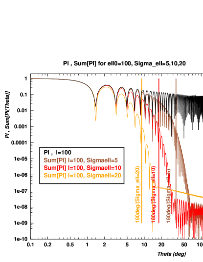
Figure 3: Legendre Polynomial and $Q_{L}=\sum P_{\ell}$ functions, plotted for $L=100$ and $\sigma_{\ell}=5,10,20$. We have plotted $|P_{\ell}|,|Q_{L}|)$. Notice also that both axes have logarithmic scales.

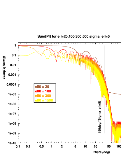
Figure 4: Legendre Polynomial $|P_{\ell}|$ and and the $|Q_{L}|$functions, plotted for $\sigma_{\ell}=5$, and $\ell 0=20,100,200,1500$. Notice that both axes have logarithmic scales.

3.3 Partial maps : Decomposition on the $Y_{\ell}^{m}$ basis

As we mentioned in section 2, a signal defined as a function of direction can be decomposed in spherical harmonics (see equation (1)). Optimized algorithms for performing numerically this decomposition on pixelized spherical maps are commonly used in analyzing CMB data (Muciaccia et al (1997) , Gorski et al (2005)). The computed $a_{{\ell}{m}}$ coefficients are used to derive the angular power spectrum $\widehat{C}_{\ell}$ using equation (4). When an incomplete (or partial) sky map is expanded on the $Y_{\ell}^{m}$ basis, the resulting power spectrum suffers systematic effects and is often called a $\mathrm{pseudo-}C_{\ell}$ spectrum. The $\mathrm{pseudo-}C_{\ell}$ spectrum distortion has already been studied by several authors and can be found for example in (Hivon et al (2002), Magneville & Pansart (2007)). The partial map can be written as the result of applying a mask on the original signal. One can then show that the $\tilde{a}_{\ell m}$ coefficients computed on the masked map can be related to the true $a_{{\ell}{m}}$ through a linear relation, which can be written in matrix form:

$$s^{p}(\theta,\phi) = s(\theta,\phi)\times\mathrm{mask}(\theta,\phi)$$ (17)

$$\left[\tilde{a}_{\ell m}\right] = \left[\left[\mathbf{A}\right]\right]*\left[a_{\ell m}\right]$$ (18)

The above relation is completely general, independent of the statistical properties of the signal $s(\theta,\phi)$ and valid for each realization. The $\left[\left[\mathbf{A}\right]\right]$ matrix coefficients depend on the mask spherical harmonic decomposition and Clebsch-Gordan coefficients. Then, using the isotropy of the signal, it is possible to compute the coupling matrix $\left[\left[\mathbf{B_{\ell\ell^{\prime}}}\right]\right]$ relating the $\mathrm{pseudo-}C_{\ell}$ power spectrum to the true angular power spectrum. Although $\left[\left[\mathbf{A}\right]\right]$ is a huge matrix, ($\sim 2\,10^{6}\times 2\,10^{6}$ elements for $\ell_{max}=1000$), only a small fraction of the elements contribute to the $\left[\left[\mathbf{B_{\ell\ell^{\prime}}}\right]\right]$ matrix.

$$\left[\langle\tilde{C_{\ell}^{p}}\rangle\right]\;=\;\left[\left[\mathbf{B_{\ell\ell^{\prime}}}\right]\right]*\left[C_{\ell^{\prime}}\right]$$ (19)

The computations to obtain the $\left[\left[\mathbf{B_{\ell\ell^{\prime}}}\right]\right]$ coupling matrix using the above method are rather tedious, while it is possible to compute this matrix simply by applying the formalism presented in this paper.

One can construct an estimator $\xi^{\prime}$ of the angular correlation function using equation (2) with the integrals limited to the partial map where the function $s(\vec{\Omega})$ is measured. A lengthy computation (Magneville & Pansart, 2007) shows that this estimator is unbiased for separation angles $\gamma<\gamma_{max}$. However a fast computation of the angular correlation function uses equation (6) or its linear form (9) and the full sphere function should be used. This corresponds to equation (2) with integrals on the full sphere $S^{2}\times S^{2}$ putting $s(\vec{\Omega})=0$ when $\vec{\Omega}$ is not pointing to the “observed” partial map. This estimator (noted $\hat{\xi}^{p}$), which is of course highly biased, will be the one used hereafter.

As $\xi^{\prime}$ and $\hat{\xi}^{p}$ are related by a multiplication by the correlation function $\xi^{\mathrm{mask}}(\gamma)$ of the mask itself, we can notice that the average of the angular correlation function ($\hat{\xi}^{p}$) computed on the masked sphere is related to the correlation function of the complete sphere by:

$$\langle\xi^{\prime}(\gamma)\rangle = \xi(\gamma)\hskip 5.69054pt\mathrm{(unbiased\,estimator)}$$

$$\hat{\xi}^{p}(\gamma) = \xi^{\mathrm{mask}}(\gamma)\times\xi^{\prime}(\gamma)$$

$$\langle\hat{\xi}^{p}(\gamma)\rangle = \xi^{\mathrm{mask}}(\gamma)\times\xi(\gamma)$$

Here, $\;\xi^{\mathrm{mask}}(\gamma)$ can easily be computed using equation (6) and the optimized algorithms cited below, applied to the mask. The distortion matrix in relation (11) can then simply be written as a diagonal matrix $D^{\mathrm{mask}}$ which can be used to compute the $\left[\left[\mathbf{B_{\ell\ell^{\prime}}}\right]\right]$.

$$D^{\mathrm{mask}}(i,i) = \xi^{\mathrm{mask}}(\gamma_{i})$$ (20)

$$\left[\left[\mathbf{B_{\ell\ell^{\prime}}}\right]\right] = \left[\left[\mathbf{K}\right]\right]^{-1}*\left[\left[\mathbf{D^{mask}}\right]\right]*\left[\left[\mathbf{K}\right]\right]$$

Figure 5 illustrates the distortion of the angular correlation function estimated from $\tilde{a}_{\ell m}$ coefficients computed on the masked map. The undistorted angular correlation function correponding to a WMAP-like $C_{\ell}$ power spectrum, the mean value of the distorted correlation function $\langle\widetilde{\xi}\rangle$ and the mask correlation function $\xi^{\mathrm{mask}}(\gamma)$ are plotted as a function of the $\gamma$ angle, for a partial $30^{\circ}\times 30^{\circ}$ map.

The analysis of the coupling matrix $\left[\left[\mathbf{B_{\ell\ell^{\prime}}}\right]\right]$ shows that the $\ell$-space resolution of $\mathrm{pseudo-}C_{\ell}$ spectrum is compatible with the optimal resolution $\Delta\ell\sim\pi/\gamma_{max}$, but has long tails or correlation lengths. These long tails are responsible for the systematic shifts of $\mathrm{pseudo-}C_{\ell}$ spectrum relative to the true one. This can be seen on figure 6 below, showing a row of the coupling matrix $B_{\ell\ell^{\prime}}$ for $\ell=\ell_{0}=300$.

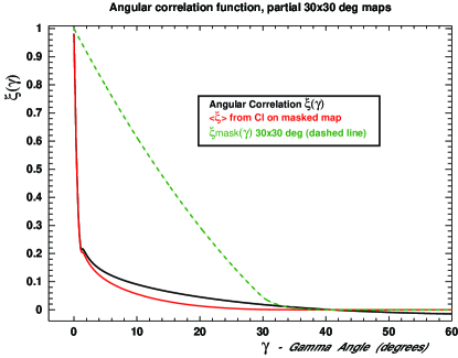
Figure 5: Distortion of the angular correlation function when computed from spherical harmonic decomposition of a partial (masked) spherical map. The partial map has a $30^{\circ}$ extension on each of the two orthonal directions. Rescaled $\xi(\gamma)$ (black) and the distorted $\langle\widetilde{\xi}\rangle$ (red) are shown for a WMAP-like angular power spectrum, as well the ratio $\xi^{\mathrm{mask}}(\gamma)=\langle\widetilde{\xi}\rangle/\xi^{\mathrm{mask}}(\gamma)$ (dashed green). Notice that the angular $\gamma$ range is limited to $60^{\circ}$ on the figure.

3.4 Partial maps : Correcting $\mathrm{pseudo-}C_{\ell}$ spectrum

In some sense, the correlation function $\widetilde{\xi}(\gamma)$ obtained through the $\mathrm{pseudo-}C_{\ell}$ computation applies a weighting function ($\xi^{\mathrm{mask}}$) which is inversely proportional to the number of available measurement ($s(\theta,\phi)$) pairs i.e., to the statistical significance of the partial sphere correlation function. It is possible to obtain the unbiased correlation function by applying the inverse correction $1/\xi^{\mathrm{mask}}$ to the correlation function of the masked sphere, up to a maximum angle $\gamma_{max}$ which should be less than the maximum extent of the partial map. As we increase $\gamma_{max}$, the statistical errors on the corrected angular correlation function, and the corrected angular power spectrum increase. There is thus a tradeoff between the $\ell$-space resolution and the statistical uncertainties of the recovered power spectrum $\widehat{C}_{\ell}$.

The statistical uncertainties (variance) associated with the recovered $\xi$ or $C_{\ell}$, depend on the true power spectrum and can not be computed using the formalism described here. It is however possible to compute the variance for specific partial map shapes, such as polar cap maps (see Magneville & Pansart (2007)). In this paper, we have computed theses uncertainties using Montecarlo simulation and the corresponding results are presented in the next section. In figure 6, the $\mathrm{pseudo-}C_{\ell}$ window function is compared to the one obtained for the corrected $C_{\ell}$ for two values of $\gamma_{max}$ ($30^{\circ},\;36^{\circ}$). On partial $30^{\circ}\times 30^{\circ}$, the maximum possible value for $\gamma_{max}\sim\sqrt{2}\times 30^{\circ}\sim 42^{\circ}$. Using a correction up to $\gamma_{max}=36^{\circ}$, we obtain statistical errors comparable to those associated with the $\mathrm{pseudo-}C_{\ell}$, while significantly decreasing the systematic effects on the recovered power spectrum (See section 4 ).

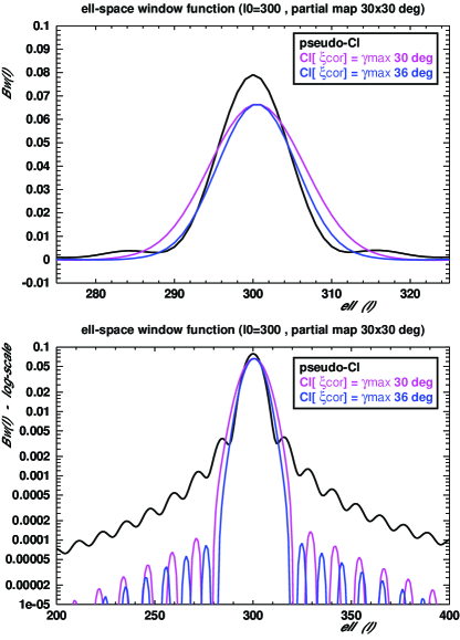
Figure 6: $30^{\circ}\times 30^{\circ}$ partial map : Comparison of $B_{\ell\ell^{\prime}}$ matrix row for $\ell=300$ (black) with Gaussian weighted $C^{t}(\ell)$ estimated from $\xi^{t}(\gamma)$, truncated at $\gamma_{max}=30^{\circ}$ (magenta) and $\gamma_{max}=36^{\circ}$ (Top: linear Y-scale, bottom: logarithmic Y-scale).

We propose the following procedure to recover an unbiased or corrected power spectrum, using fast spherical harmonic decomposition of masked spherical maps.

1. Compute the $\mathrm{pseudo-}C_{\ell}$ angular power spectrum on the masked sphere $\widehat{C}_{\ell}^{p}$ through fast spherical harmonic decomposition, as well as the $\mathrm{pseudo-}C_{\ell}$ of the the mask itself.

2. Compute the corresponding discrete angular correlation function and the mask correlation function

   $$\begin{array}[]{lcl}\left[\hat{\xi}^{p}(\gamma_{i})\right]&=&\left[\left[\mathbf{K}\right]\right]*\left[\widehat{C}_{\ell}^{p}\right]\\ \left[\xi^{\mathrm{mask}}(\gamma_{i})\right]&=&\left[\left[\mathbf{K}\right]\right]*\left[C_{\ell}^{\mathrm{mask}}\right]\par\end{array}$$ (21)

3. Define the truncation angle $\gamma_{max}$ compatible with the maximum map extent and desired $\ell$ resolution. Compute the corrected-truncated angular correlation function using the diagonal correction matrix $\mathbf{Dcor}$.

   $$\begin{array}[]{lcl}\left[\hat{\xi}^{t}(\gamma_{i})\right]&=&\left[\left[\mathbf{Dcor}\right]\right]*\left[\hat{\xi}^{p}(\gamma_{i})\right]\\ \mathrm{Dcor(i,i)}&=&1/\xi^{\mathrm{mask}}(\gamma_{i})\hskip 5.69054pt\gamma_{i}\leq\gamma_{max}\\ \mathrm{Dcor(i,i)}&=&0\hskip 5.69054pti\neq j\,\mathrm{or}\,\gamma_{i}>\gamma_{max}\end{array}$$ (22)

   The correction matrix is equal to the inverse of the mask distortion (see equation (20)) if angular correlation information is present up to $\gamma_{max}=\pi$. It is useful to apply a step smoothing function to avoid the discontinuity of $\hat{\xi}^{t}$ for $\gamma=\gamma_{max}$, such as a sigmoid:

   $$f(\gamma)=1/\left[1+\exp\left(\frac{\gamma-\gamma_{max}}{\delta}\right)\right]\hskip 5.69054pt\mathrm{with}\hskip 5.69054pt\delta\sim 0.01\gamma_{max}$$

   This step smoothing function enhances the behavior of the computed power spectrum, decreasing residual oscillations.

4. Compute the corrected angular spectrum and apply the Gaussian filter function in $\ell$-space with $\sigma_{\ell}=\pi/\gamma_{max}$.

   $$\begin{array}[]{lcl}\left[\widehat{C}_{\ell}^{t}\right]&=&\left[\left[\mathbf{K^{-1}}\right]\right]*\left[\hat{\xi}^{t}(\gamma_{i})\right]\\ \left[\widehat{C}_{\ell}^{t}\right]&=&\left[\left[\mathbf{W_{G}}\right]\right]*\left[\widehat{C}_{\ell}^{t}\right]\\ \mathrm{W_{G}(\ell_{0},\ell)}&=&=\frac{\exp((\ell-\ell_{0})^{2}/2\sigma_{\ell}^{2})}{\sum_{\ell}\exp((\ell-\ell_{0})^{2}/2\sigma_{\ell}^{2})}\end{array}$$ (23)

The coupling matrix $\mathrm{B_{c}}$ is independent of the true power spectrum and can be computed using the following relation:

$$\begin{array}[]{lcl}\langle\left[\widehat{C}_{\ell}^{t}\right]\rangle&=&\left[\left[\mathbf{B_{c}}\right]\right]*\left[C_{\ell}\right]\\ \left[\left[\mathbf{B_{c}}\right]\right]&=&\left[\left[\mathbf{W_{G}}\right]\right]*\left[\left[\mathbf{K^{-1}}\right]\right]*\left[\left[\mathbf{Dcor}\right]\right]*\left[\left[\mathbf{K}\right]\right]\end{array}$$ (24)

4 Simulation results on small maps and masked maps

There is a tradeoff between the achievable resolution and the uncertainties of the estimated power spectrum. In order to evaluate these uncertainties, we have performed Montecarlo simulations to generate partial and full sky spherical maps and compute the power spectrum using spherical harmonic decomposition and the corrected/truncated angular auto correlation function. The method to correct systematic effects proposed in this work is independent of the true power spectrum. The computation of the coupling matrix and correction matrix is rather fast with a CPU time comparable to few Monte-Carlo realisations using fast spherical harmonics map analysis ($\sim$ minute). Reasonable estimates of errors for a given input power spectrum can be obtained using few hundred realisations. Although it is possible to compute the systematic effects due to the limited sky coverage using Monte-Carlo, this would require much larger computation time compared to the uncertainty estimates. The estimate of the $\left[\left[\mathbf{B_{\ell\ell^{\prime}}}\right]\right]$ coupling matrix elements with sufficient precision would need a large number of Monte-Carlo realisations, due to the cosmic variance. In addition, this computation process would have to be repeated for several input power spectra.

The simulations have been performed with different partial map geometries and input (true) $C_{\ell}$ power spectra to check the validity of the conclusions. However, for the sake of clarity, we present here the results only for two map geometries and two input spectra. We have used WMAP-like true $C_{\ell}$ power spectrum, labeled $t_{wmap}$ and a second shape, labeled $t_{6}$, which have sharp features on top of a smooth spectrum $C(\ell)=Cte/[\ell\times(\ell+1)]+\mathrm{peaks}$ in order to illustrate the $\ell$-space resolution effect. The results presented here have been obtained for the following two map geometries:

1. Partial square map, $30^{\circ}\times 30^{\circ}$, covering the angular range $75^{\circ}\leq\theta\leq 105^{\circ}$ and $\phi_{0}\leq\phi\leq\phi_{0}+30^{\circ}$. This map covers $\sim 0.27\;sr\;=\;0.022\;\times\;4\pi\;sr$. This small map corresponds to the case of ground or balloon CMB instruments.

2. A nearly complete spherical map, but with an equatorial band removed (set to zero). This case shows the distortion of the $C(\ell)$ power spectrum obtained from all sky space experiments such as WMAP or Planck, where some part of the sky with strong non-CMB microwave signals has to be masked. The removed equatorial band illustrates the effect of Galactic cut applied to CMB maps. We have performed simulations on $4\pi$ spherical maps with a $\Delta\theta=\pm 10^{\circ}$ equatorial band cut ($s(\theta,\phi)=0$ for $80^{\circ}\,<\theta<100^{\circ}\;,\forall\phi$). Such a map covers 82.5 % of the whole sky ($0.825\times 4\pi\;sr$) and provides correlation information for the whole angular range ($0\leq\gamma\leq\pi$).

3. A more realistic case where we have applied the 5-year WMAP CMB temperature analysis (KQ85) mask (Gold et al, 2008) to simulated CMB maps. The mask and corresponding normalised correlation function is shown in figure 7. The unmasked area corresponds to $\sim 0.82\times 4\pi\;sr$, nearly equal to the area of maps with a $\pm 10^{\circ}$ equatorial band removed. It has a complex and patchy shape.

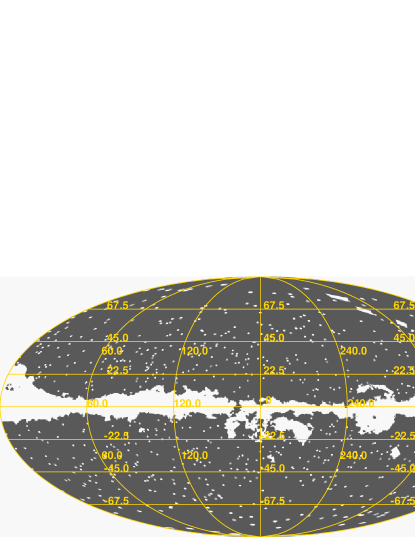
Figure 7: WMAP KQ85 CMB temperature analysis mask (top) and the corresponding normalised correlation function $\xi^{\mathrm{mask}}(\gamma)$ (bottom).

Given the overall shape of the $C_{\ell}$ spectra studied here, we have represented $\ell\times(\ell+1)\,C_{\ell}$ for the power spectrum, and $\ell\times(\ell+1)\,\sigma_{C_{\ell}}$ for the associated statistical uncertainties on all figures that follow in this section. The systematic shifts of the recovered power spectrum can be quantified using difference between the recovered and true power spectrum, normalised to the cosmic variance $\sigma_{cv}(\ell)$

$$\delta(\ell)=\frac{\langle\widehat{C}_{\ell}\rangle-C_{\ell}}{\sigma_{cv}(\ell)}$$

4.1 Small $30^{\circ}\times 30^{\circ}$ maps

The figures 8 and 9 show the recovered power spectrum on small $30^{\circ}\times 30^{\circ}$ maps for a true WMAP-like power spectrum. The systematic shifts of the $\mathrm{pseudo-}C_{\ell}$ power spectrum are clearly visible, in particular on figure 9 (top). The false oscillations on the raw power spectrum recovered from truncated $\xi$ is also shown on the figure 8 (top).

It can also be seen that by choosing $\gamma_{max}=36^{\circ}$, it is possible to avoid nearly all the systematic shifts of the power spectrum, while keeping the level of statistical fluctuations comparable to the $\mathrm{pseudo-}C_{\ell}$, and without losing the $\ell$-space resolution (See figure 9 and 10). However, it should also be noted that the corrected $C_{\ell}$ suffers a systematic overestimation at low $\ell\lesssim\left(2-3\times\sigma_{\ell}=2-3\pi/\gamma_{max}\right)$, as expected from the coupling matrix $\mathrm{B_{c}}$.

The systematic shift $\delta(\ell)$ decreases by a factor 10-30, changing from $\delta\sim 0.25-0.75$ in the case of $\mathrm{pseudo-}C_{\ell}$ to less than 0.05 for Gaussian weighted $C_{\ell}^{t}$ computed from $\xi(\gamma)$ corrected up to $\gamma_{max}=36^{\circ}$ (figure 9).

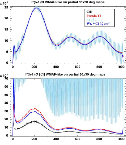
Figure 8: $30^{\circ}\times 30^{\circ}$ partial maps : Comparison of computed power spectrum and true $t_{wmap}$ power spectrum (top) and the associated statistical errors (bottom). True power spectrum in black, $\mathrm{pseudo-}C_{\ell}$ in red, $C_{\ell}^{t}$ computed from corrected angular correlation function truncated at $\gamma_{max}=30^{\circ}$ (light blue), and corrected $C(\ell)^{t}$ binned with Gaussian weights (blue)

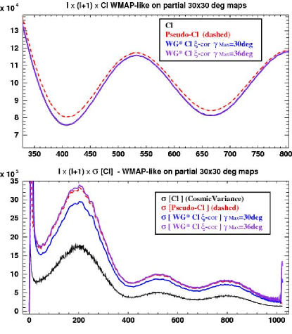
Figure 9: $30^{\circ}\times 30^{\circ}$ partial maps : Comparison of computed power spectrum and true $t_{wmap}$ power spectrum (top) and the associated statistical errors (bottom). True power spectrum in black, $\mathrm{pseudo-}C_{\ell}$ in red, Gaussian weighted binned $C_{\ell}^{t}$ computed from corrected angular correlation function truncated at $\gamma_{max}=30^{\circ}$ (blue), and with $\gamma_{max}=36^{\circ}$ (violet)

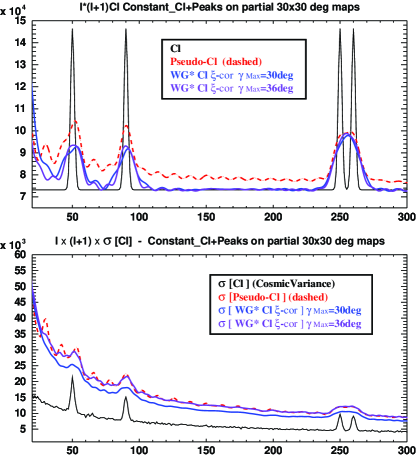
Figure 10: $30^{\circ}\times 30^{\circ}$ partial maps : Comparison of computed power spectrum and true $t_{6}$ power spectrum (top) and the associated statistical errors (bottom). True power spectrum in black, $\mathrm{pseudo-}C_{\ell}$ in red, Gaussian weighted binned $C_{\ell}^{t}$ computed from corrected angular correlation function truncated at $\gamma_{max}=30^{\circ}$ (blue), and with $\gamma_{max}=36^{\circ}$ (violet)

4.2 Maps with $\pm$ $10^{\circ}$ Galactic cut

The figure 11 shows the bias introduced on the recovered power spectrum, specially at low multipoles $\ell\lesssim 30$ using uncorrected $\widehat{C}_{\ell}^{p}$ from map projection on the $Y_{\ell}^{m}$ basis. In this case, the angular correlation function can be estimated at all angular scales, but the $\widetilde{\xi}(\gamma)$ obtained from the $\mathrm{pseudo-}C_{\ell}$ is distorted. By correcting the $\widetilde{\xi}(\gamma)$, it is possible to recover the unbiased power spectrum $\widehat{C}_{\ell}^{\hat{\xi}}$, as shown on figure 11 (top). The systematic shift $\delta(\ell)$ changes from $\delta\sim 0.25$ in the case of $\mathrm{pseudo-}C_{\ell}$ to less than 0.05 for Gaussian weighted $\widehat{C}_{\ell}$ computed from corrected $\xi(\gamma)$. However, the statistical fluctuations are larger, compared to the cosmic variance, reachable if the complete $4\pi$ map is available, or to the $\mathrm{pseudo-}C_{\ell}$ variance on the cut map. Figure 12 shows the effect of the equatorial cut on a sharp feature present in the simulated power spectrum around $\ell=50$. The power spectrum computed from corrected angular autocorrelation also corrects this distortion.

Although more sophisticated methods can be used to recover the spectrum at low multipoles from cut maps, the correction algorithm proposed here can be used to easily correct the $\mathrm{pseudo-}C_{\ell}$ spectrum.

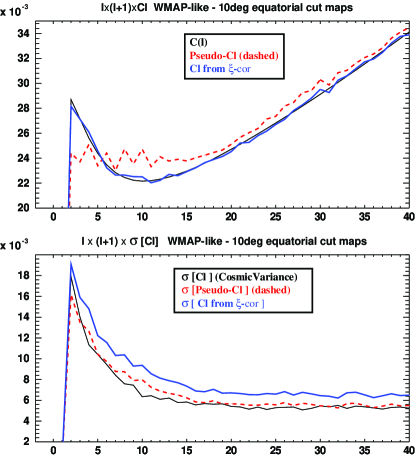
Figure 11: $4\pi$ maps with $\pm\;10^{\circ}$ equatorial cut: Comparison of computed power spectrum and true $t_{wmap}$ power spectrum (top) and the associated statistical errors (bottom). True power spectrum in black, $\mathrm{pseudo-}C_{\ell}$ in red, Gaussian weighted binned $C_{\ell}^{\xi c}$ computed from corrected angular correlation function in blue.

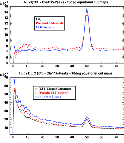
Figure 12: $4\pi$ maps with $\pm\;10^{\circ}$ equatorial cut: Comparison of computed power spectrum and true $t_{6}\;$ ($C(\ell)=\mathrm{Cte}/\ell\times(\ell+1)+\mathrm{peaks}$) power spectrum (top) and the associated statistical errors (bottom). True power spectrum in black, $\mathrm{pseudo-}C_{\ell}$ in red, $C_{\ell}^{\xi c}$ computed from corrected angular correlation function in blue

4.3 Maps with WMAP KQ85 mask

The effect of the WMAP KQ85 foreground suppression mask on the recovered power spectrum is shown in figure 13. This mask cuts an equatorial area on the map which is significantly less extended than in the case of the simple $\pm$ $10^{\circ}$ cut discussed above, but it removes also a large number of smaller patches of the sky scattered over the map. As a result, it can be seen that the systematic effects at low multipoles on the recovered $\mathrm{pseudo-}C_{\ell}$ are smaller compared to the more extended $\pm\;10^{\circ}$ equatorial cut, while significant shift appears at higher multipoles, around $\ell=400$ for instance, due to the patchy structure of the mask. This patchy structure is also responsible for the oscillatory behaviour of the $C_{\ell}^{\xi c}$ power spectrum computed from the corrected angular correlation function, for $\ell\gtrsim 10$. Theses unphysical oscillations can be smoothed out by applying a narrow Gaussian ($\sigma_{\ell}=0.75$) filter function, $C_{\ell}^{\xi c,G}$, as can be seen on figure 13.

As expected, correcting $\xi(\gamma)$ using $\xi^{\mathrm{mask}}(\gamma)$ increases the statistical uncertainties compared to $\mathrm{pseudo-}C_{\ell}$, while the filtered power spectrum has smaller variance. It is possible to use the combined power spectrum, $C_{\ell}^{\xi c}$ without filtering for $\ell\lesssim 10$ and Gaussian weighted $C_{\ell}^{\xi c,G}$ for $\ell\gtrsim 10$. The systematic shift $\delta(\ell)$ decreases from $\delta\sim 0.5-1.5$ in the case of $\mathrm{pseudo-}C_{\ell}$ to $\delta\lesssim 0.05$ for this combined $\widehat{C}_{\ell}$.

We have also checked that our conclusions are valid in the presence of noise. We have performed simulations where Gaussian fluctuations, with smooth spatial variations have been added to simulated maps. The reconstructed power spectrum corresponds to the sum of the sky signal and the noise spectra ($\widehat{C}_{\ell}=C_{\ell}+C_{\ell}^{\mathrm{noise}}$), distorted by the mask, as it is expected for nearly isotropic uncorrelated noise.

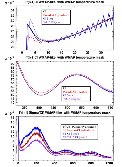
Figure 13: $4\pi$ maps masked with the WMAP 5 year temperature KQ85 mask. Comparison of recovered power spectrum and true $t_{wmap}$ power spectrum (top and middle) and the associated statistical errors (bottom). True power spectrum in black, $\mathrm{pseudo-}C_{\ell}$ in red, dashed, $C_{\ell}^{\xi c}$ computed from corrected angular correlation function in blue, and filtered with Gaussian weights ($\sigma_{\ell}=0.75$) in violet $C_{\ell}^{\xi c,G}$.

5 Conclusions

We have established a simple method to evaluate and correct systematic effects associated with power spectrum computed using the $\mathrm{pseudo-}C_{\ell}$ on partial maps. The coupling matrix $B_{\ell\ell^{\prime}}$ can indeed be computed using matrix algebra and the sky mask spherical harmonic decomposition. We have also described an algorithm to correct the systematic shifts of the calculated power spectrum, as well as a near optimal $\ell$-space window or filter function. It should be noted that it is possible to improve the $\ell$ resolution, compared to the natural resolution $\Delta\ell\sim\sigma_{\ell}\sim\pi/\gamma_{max}$ at the expense of higher statistical fluctuations. For all sky CMB experiments such as WMAP or Planck, non-CMB dominated parts of the sky (galaxy …) are usually excluded from the angular power spectrum estimation. We show that our method can be used to correct the power spectrum distortions at low $\ell$ in such cases, when the angular power is computed using fast spherical harmonic decomposition on almost complete maps.

The correction method described here can easily be extended to the CMB-polarisation power spectrum. A similar approach for polarised maps has been developed in (Chon et al, 2004). It should also be possible to use this method to improve the angular power spectrum calculation by taking into account individual pixel measurement errors. For observations with negligible correlated noise, a weighting function mask inversely proportional to the individual pixel measurement uncertainties can be applied to the map before decomposition on the $Y_{\ell m}$ basis, and subsequently corrected for.

Appendix

We will show that one can invert equation (9) for a certain choice of the separation angles $\gamma$. We assume that the power at large $\ell$ is negligible. We can then consider that $C_{\ell}=0$ for all multipoles with $\ell>\ell_{max}$. The sum in equation (6) becomes finite, so for $n_{\gamma}$ given discrete values of $\gamma$, the matrix elements in equation (9) are:

$$[[K]]_{i\ell}\;=\;\frac{2\ell+1}{4\pi}\;P_{\ell}(\cos(\gamma_{i}))$$ (25)

with   $1\leq i\leq n_{\gamma}$   and   $0\leq\ell\leq\ell_{max}$.

If the matrix $[[K]]$ is invertible, one may write $\;[C_{\ell}]=[[K]]^{-1}*[\xi_{i}]\;$ and the $C_{\ell}$ spectrum can be recovered from the values of the angular correlation function computed at angular separations $\gamma_{i}$.
In the following we will show that the separation angles $\gamma_{i}$ can be choosen such that the square matrix is non-singular.

$P_{\ell}(x=\cos(\gamma))$ is a polynomial of degree $\ell$ in the interval $[-1,+1]$. Using equation (6) we see that $\xi(\gamma)$ is a polynomial of degree at most $\ell_{max}$. The integrand $\xi\times P_{\ell}$ of equation (7) is a polynomial of degree at most $\ell_{max}+l$, so for the highest multipole $C_{\ell_{max}}$ the integrand has a degree at most $2\ell_{max}$.

We know that, using Gauss-Legendre quadrature of order $n$, integrals of polynomials of degree up to $2n+1$ can be exactly expressed as a $n$-term weighted sum of the polynomials computed at special values of $x$ (see  Abramowitz et al (1972)).

For all $\ell\leq\ell_{max}$ and for $L\geq\ell_{max}+1$, the integral in equation (7) can be expressed as the algebraic sum:

$$C_{\ell}\;=\;2\pi\;\underset{i=1}{\overset{L}{\sum}}\;\xi(\gamma_{i})P_{\ell}(\cos(\gamma_{i}))\times\;w_{i}$$ (26)

where $x_{i}=\cos(\gamma_{i})$ are the $L$ roots of $P_{L}(x)$ and $w_{i}$ the weights. For $L\geq\ell_{max}+1$, this can be written in a matrix form:

$$\begin{array}[]{rclcl}[C_{\ell}]&=&[[K^{\prime}]]*[\xi_{i}]&&0\leq\ell\leq\ell_{max}\\ &&&&\\ K^{\prime}_{\ell i}&=&2\pi P_{\ell}(\cos(\gamma_{i}))\times\;w_{i}&&1\leq i\leq L\end{array}$$

Clearly, if we take $L=\ell_{max}+1$, the number of abscissas values is $n_{\gamma}=\ell_{max}+1$ and the matrix $[[K]]$ is square. In that case $[[K^{\prime}]]=[[K]]^{-1}$ and equation (7) can be written

$$[C_{\ell}]=[[K]]^{-1}*[\xi_{i}]\quad\left(1\leq i\leq\ell_{max}+1,\;0\leq\ell\leq\ell_{max}\right)$$ (27)

Remark: Numerically, the angular correlation function could also be computed at $\ell_{max}+1$ regularly spaced values $\gamma_{i}$ between $0$ and $\pi$. This is possible because the $\gamma_{i}$ corresponding to the Legendre polynomial roots $x_{i}=\cos(\gamma_{i})$ satisfy the relation

$$\frac{2i-1}{2\ell+1}\;\leq\;\frac{\gamma_{i}}{\pi}\;\leq\;\frac{2i+1}{2\ell+1}\qquad\text{for}\quad P_{\ell}(\cos(\gamma))$$ (28)

and are nearly regularly spaced.

Thus the angular distance between a Legendre polynomial root and the nearest regularly spaced abscissa is always lower than the resolution associated with the highest multipole ($\sim\pi/\ell_{max}$).

References

Abramowitz et al (1972)
M.Abramowitz and I.Stegun,
Handbook of Mathematical Functions (10th ed.), p.877, eq.25.4.29 (ISBN 0-486-61272-4)
Benoit et al (2003)
Benoit A., et al, 2003, A&A, 399, L19
Carlstrom et al (2003)
Carlstrom J. E., Kovac J., Leitch E.M., Pryke C., 2003, NewAR, 47, 953
Chon et al (2004)
Chon et al, 2004, MNRAS 350, 914
Das et al (2009)
Das S., Hajian A., Spergel D., 2009, Phys.Rev D 79, 083008, arXiv:0809.1092
Fowler et al (2010)
Fowler W., et al, 2010, arXiv:1001.2934
Gold et al (2008)
Gold B., et al., 2009, ApJS, 180, 265
Gorski et al (2005)
Gorski K.M., Hivon E., Banday A.J., 2005, ApJ, 622, 759
Hansen et al (2005)
Hansen F.K., Gorski K.M., Hivon E., 2002, MNRAS, 336, 1304
Hivon et al (2002)
Hivon E., Gorski K.M., Netterfield C.B., Crill B.P.,
Prunet S., Hansen F., 2002, ApJ, 567 Issue 1, 2
Hu & Dodelson (2002)
Hu W., Dodelson S., 2002, ARAA, 40, 171
Jones et al (2006)
Jones W.C., et al, 2006, ApJ, 647, 823
Larson et al (2010)
Larson D., Dunkley J., Hinshaw G., et al, 2010, ApJS (submitted, arXiv:1001.4635)
Lee et al (2001)
Lee A.T., et al, 2001, ApJ Lett., 561, L1
Lueker et al (2009)
Lueker M., et al, 2009, arXiv:0912.4317