The Electrosphere of Macroscopic “Quark Nuclei”:
A Source for Diffuse MeV Emissions from Dark Matter.

Abstract

Using a Thomas-Fermi model, we calculate the structure of the electrosphere of the quark antimatter nuggets postulated to comprise much of the dark matter. This provides a single self-consistent density profile from ultrarelativistic densities to the nonrelativistic Boltzmann regime that use to present microscopically justified calculations of several properties of the nuggets, including their net charge, and the ratio of MeV to 511 keV emissions from electron annihilation. We find that the calculated parameters agree with previous phenomenological estimates based on the observational supposition that the nuggets are a source of several unexplained diffuse emissions from the Galaxy. As no phenomenological parameters are required to describe these observations, the calculation provides another nontrivial verification of the dark-matter proposal. The structure of the electrosphere is quite general and will also be valid at the surface of strange-quark stars, should they exist.

I Introduction

In this paper we explore some details of a testable and well-constrained model for dark matter [1, 2, 3, 4, 5] in the form of quark matter as antimatter nuggets. In particular, we focus on physics of the “electrosphere” surrounding these nuggets: It is from here that observable emissions emanate, allowing for the direct detection of these dark-antimatter nuggets.

We first provide a brief review of our proposal in Sec. II, then describe the structure of the electrosphere of the nuggets using a Thomas-Fermi model in Sec. IV. This allows us to calculate the charge of the nuggets, and to discuss how they maintain charge equilibrium with the environment. We then apply these results to the calculation of emissions from electron annihilation in Sec. V, computing some of the phenomenological parameters introduced in [6] required to explain current observations. The values computed in the present paper are consistent with these phenomenologically motivated values, providing further validation of our model for dark matter. The present results concerning the density profile of the electrosphere may also play an important role in the study of the surface of quark stars, should they exist.

II Dark Matter as Dense Quark Nuggets

Two of the outstanding cosmological mysteries – the natures of dark matter and baryogenesis – might be explained by the idea that dark matter consists of compact composite objects (ccos) [1, 2, 3, 4, 5] similar to Witten’s strangelets [7]. The basic idea is that these ccos – nuggets of dense matter and antimatter – form at the same qcd phase transition as conventional baryons (neutrons and protons), providing a natural explanation for the similar scales $\Omega_{\textsc{dm}}\approx 5\Omega_{B}$. Baryogenesis proceeds through a charge separation mechanism: both matter and antimatter nuggets form, but the natural cp violation of the so-called $\theta$ term in qcd – which was of order unity $\theta\sim 1$ during the qcd phase transition – drives the formation of more antimatter nuggets than matter nuggets, resulting in the leftover baryonic matter that forms visible matter today (see [2] for details). Note, it is crucial for our mechanism that cp violation be able to drive charge separation: though not yet proven, this idea may already have found experimental support through the Relativistic Heavy Ion Collider (rhic) at Brookhaven [19], where charge separation effects seem to have been observed [20, 21]

The mechanism requires no fundamental baryon asymmetry to explain the observed matter/antimatter asymmetry. Together with the observed relation $\Omega_{\textsc{dm}}\approx 5\Omega_{B}$ (see [22] for a review) we have

$$B_{\text{universe}}=0 =B_{\text{nugget}}+B_{\text{visible}}-\bar{B}_{\text{antinugget}}$$ (1a)

$$B_{\text{dark-matter}} =B_{\text{nugget}}+\bar{B}_{\text{antinugget}}\approx 5B_{\text{visible}}$$ (1b)

where $B_{\text{universe}}$ is the overall asymmetry – the total number of baryons minus the number of antibaryons in the Universe – and $B_{\text{dark-matter}}$ is the total number of baryons plus antibaryons hidden in the dark-matter nuggets. The dark matter comprises a baryon charge of $B_{\text{nugget}}$ contained in matter nuggets, and an antibaryonic charge of $\bar{B}_{\text{antinugget}}$ contained in antimatter nuggets. The remaining unconfined charge of $B_{\text{visible}}$ is the residual “visible” baryon excess that forms the regular matter in our Universe today. Solving Eq. (1) gives the approximate ratios $\bar{B}_{\text{antinugget}}$:$B_{\text{nugget}}$:$B_{\text{visible}}\simeq$ 3:2:1.

Unlike conventional dark-matter candidates, dark-matter/antimatter nuggets will be strongly interacting, but macroscopically large, objects. They do not contradict any of the many known observational constraints on dark matter or antimatter [3] for three reasons:

1. They carry a huge (anti)baryon charge $|B|\approx 10^{20}$ – $10^{30}$, so they have an extremely tiny number density. This explains why they have not been directly observed on earth. The local number density of dark-matter particles with these masses is small enough that interactions with detectors are exceedingly rare and fall within all known detector and seismic constraints [3]. (See also [23, 24] and references therein.)

2. The nugget cores are a few times nuclear density $\rho\sim 10$ GeV$/$fm³, and thus have a size $R\sim 10^{-7}$–$10^{-3}$ cm. Their interaction cross section is thus small $\sigma/M\approx 4\pi R^{2}/M=10^{-13}$–$10^{-9}$ cm²/g: well below the typical astrophysical and cosmological limits, which are on the order of $\sigma/M<1$ cm²/g. Dark-matter–dark-matter interactions between these nuggets are thus negligible.

3. They have a large binding energy such that the baryonic matter in the nuggets is not available to participate in big bang nucleosynthesis (bbn) at $T\approx 1$ MeV. In particular, we suspect that the core of the nuggets forms a superfluid with a gap of the order $\Delta\approx 100$ MeV, and critical temperature $T_{c}\sim\Delta/\sqrt{2}\approx 60$ MeV, as this scale provides a natural explanation for the observed photon to baryon ratio $n_{B}/n_{\gamma}\sim 10^{-10}$ [2], which requires a formation temperature of $T_{\text{form}}=41$ MeV [25].

Thus, on large scales, the nuggets are sufficiently dilute that they behave as standard collisionless cold dark matter (ccdm). When the number densities of both dark and visible matter become sufficiently high, however, dark-antimatter–visible-matter collisions may release significant radiation and energy. In particular, antimatter nuggets provide a site at which interstellar baryonic matter – mostly hydrogen – can annihilate, producing emissions that should be observable from the core of our Galaxy of calculable spectra and energy. These emissions are not only consistent with current observations, but naturally explain several mysterious diffuse emissions observed from the core of our Galaxy, with frequencies ranging over 12 orders of magnitude.

Although somewhat unconventional, this idea naturally explains several coincidences, is consistent with all known cosmological constraints, and makes testable predictions. Furthermore, this idea is almost entirely rooted in conventional and well-established physics. In particular, there are no “free parameters” that can be – or need to be – “tuned” to explain observations: In principle, everything is calculable from well-established properties of qcd and qed. In practice, fully calculating the properties of these nuggets requires solving the fermion many-body problem at strong coupling, so we have generally resorted to “fitting” a handful of phenomenological parameters from observations. In this paper we examine the qed physics of the electrosphere, providing a microscopic basis for some of these parameters. Once these parameters are determined, the model makes unambiguous predictions about other processes ranging over more than 10 orders of magnitude in scale.

The basic picture involves the antimatter nuggets – compact cores of nuclear or strange-quark matter (see Sec. III) surrounded by a positron cloud with a profile as calculated in Sec. IV. Incident matter will annihilate on these nuggets producing radiation at a rate proportional to the annihilation rate, thus scaling as the product $\rho_{\textsc{v}}(\vec{\bm{r}})\rho_{\textsc{dm}}(\vec{\bm{r}})$ of the local visible and dark-matter densities. This will be greatest in the core of the Galaxy. To date, we have considered five independent observations of diffuse radiation from the core of our Galaxy:

1. Spi/integral (the spi instrument on the integral satellite) observes 511 keV photons from positronium decay that is difficult to explain with conventional astrophysical positron sources [26, 27, 28]. Dark-antimatter nuggets would provide an unlimited source of positrons as suggested in [29, 30].

2. Comptel/crgo (the comptel instrument on the Compton Gamma Ray Observatory (crgo) satellite) detects a puzzling excess of 1–20 MeV $\gamma$-ray radiation. It was shown in [6] that the direct $e^{+}e^{-}$ annihilation spectrum could nicely explain this deficit, but the annihilation rates were crudely estimated in terms of some phenomenological parameters. In this paper we provide a microscopic calculation of these parameters (Eqs. (19) and (21)), thereby validating this prediction.

3. Chandra (the Chandra x-ray observatory) observes a diffuse keV x-ray emission that greatly exceeds the energy from identified sources [31]. Visible-matter/dark-antimatter annihilation would provide this energy. It was shown in [4] that the intensity of this emission is consistent with the 511 keV emission if the rate of proton annihilation is slightly suppressed relative to the rate of electron annihilation. In Sec. IV.3 we describe the microscopic nature of this suppression.

4. Egret/crgo (the Energetic Gamma Ray Experiment Telescope aboard the crgo satellite) detects MeV to GeV gamma rays, constraining antimatter annihilation rates. It was shown in [4] that these constraints are consistent with the rates inferred from the other emissions.

5. Wmap (the Wilkinson Microwave Anisotropy Probe) has detected an excess of GHz microwave radiation – dubbed the “wmap haze” – from the inner $20^{\circ}$ core of our Galaxy [32, 33, 34, 35]. Annihilation energy not immediately released by the above mechanisms will thermalize, and subsequently be released as thermal bremsstrahlung emission at the eV scale. In [5] it was shown that the predicted emission from the antimatter nuggets is consistent with, and could completely explain, the observed wmap haze.

These emissions arise from the following mechanism: Neutral hydrogen from the interstellar medium (ism) will easily penetrate into the electrosphere, providing a source of electrons and protons.

The first and simplest process is the annihilation of the electrons through positronium formation, producing 511 keV photons as discussed in [29, 30]. Note that this mechanism predicts that, within the environment of the electrosphere, virtually all of the low-energy emission should be characterized by a positronium decay spectrum, including 25% as a sharp 511 keV line from the decay of the singlet state and the remaining 75% as the broad three photon continuum resulting from the triplet state. As emphasized in [36], simply postulating a dark-matter source of positrons does not suffice to explain the observed spectrum characterized by $94\pm 4\%$ positronium annihilation: The positrons must annihilate in the appropriate cool environment as provided by the electrosphere of the nuggets.

Our proposal can thus easily explain the observed 511 keV radiation. If we assume that this process is the dominant source, then we can use this to normalize the intensities of the other emissions. A remarkable feature of this proposal is that it then predicts the correct intensity for all of the other observations, even though they span many orders of magnitude in frequency.

The second process is direct annihilation of the electrons on the positrons in the electrosphere. As discussed in appendix B, the electrons are strongly screened by the positron background, and some fraction can penetrate deep within the electrosphere. There they can directly annihilate with high-momentum positrons in the Fermi sea producing radiation up to 10 MeV or so. This process was originally discussed in [6] where the ratio of direct MeV annihilation to 511 keV annihilation was characterized by several phenomenological parameters chosen to fit the observations. In Sec. V we put this prediction on solid ground and show that these parameter fits agree with the microscopic calculation based on the electrosphere structure, which depends only on qed.

The other radiation originates from the energy deposited by annihilation of the incident protons in the core of the nuggets. In [4] we argue that the protons will annihilate just inside the surface of the core, releasing some 2 GeV of energy. Occasionally this process will release GeV photons – the rate of which is consistent with the egret/crgo constraints – but most of the energy will be transferred to strongly interacting components, and ultimately about half will scatter down into $\sim 5$ MeV positrons that stream out of the core. (The $5$ MeV scale comes from the effective mass of the photon in the medium which mediates the energy exchange). These positrons are accelerated by the strong electric fields, and emit field-induced bremsstrahlung emission in the 10 keV band – a scale set by balancing the rate of emission with the local plasma frequency (photons can only be emitted once the plasma frequency is low enough). The spectrum is also calculable: It is very flat and similar to a thermal spectrum without the sharp falloff above the temperature scale. This is consistent with the Chandra observations which cannot resolve the thermal falloff, but future analysis might be able to distinguish between the two.

We shall shed some light on the interaction between the protons and the core in Sec. IV.3, but cannot yet perform the required many-body analysis to place all of this on a strong footing as this would require a practical solution to outstanding problems of high-density qcd.

The remaining energy will thermalize within the nuggets, until an equilibrium temperature of about $T\sim 1$ eV is reached [5]. Direct thermal emission at this scale would be virtually impossible to see against the backgrounds, but the spectrum – calculable entirely from qed – extends to very low frequencies, and the intensity of the emission in the microwave band is just enough to explain the wmap haze [5].

III Core Structure

A full accounting of this nugget proposal requires a proper description of the high-density phase found in the core of the nuggets. Unfortunately, a quantitative understanding of this phase requires a practical solution to the notoriously difficult problem of high-density qcd. The density of the core will be within several orders of nuclear matter density $\sim 1-100$ GeV/fm³. This is not high enough for the asymptotic freedom of qcd may be used to solve the problem perturbatively, so one must resort to nonperturbative techniques such as the lattice formulation of qcd. Unfortunately, at finite density, the presence of the infamous sign problem renders this approach exponentially expensive and it remains a famously intractable problem. As such, we cannot exactly quantify the nature of the core and must constrain its properties from other observations; we list the important properties in this section.

Fortunately, the observable emissions discussed in this paper result primarily from the calculable physical processes in the electrosphere of the nuggets, and are thus largely insensitive to the exact nature of the core. Nevertheless, the core structure must be addressed, and it is possible that future developments concerning the properties of high-density qcd could rule out the feasibility of our nugget proposal.

The first problem concerns the stability of the core. All evidence suggests that, in the absence of an external potential (such as the gravitational well of a neutron star), nuclear matter will fragment into small nuclei with a baryon number no larger than a few hundred. This suggests one of two possibilities:

• The first possibility suggested by Witten [7] is that a phase of strange-quark matter [37] becomes stable at high density. In this case, the nuggets are simply strangelets and antistrangelets and the novel feature here is that the domain walls associated with strong $CP$ violation provide the required mechanism to condense enough matter to catalyze the formation of the strangelets before they evaporate. (For a brief review, see [38] and references therein.)

  Although strangelets have not yet been observed, the possibility of stable strange-quark mater has not yet been ruled out (see for example [39]). This must be carefully reconciled with future astrophysical observations and constraints as it is conceivable that this possibility might be ruled out in the future. If the nuggets are a form of strange-quark matter, one must also consider the possibility of mixed phases as suggested in [40] (see for example [41, 42] and references therein). This would most likely have to be ruled out energetically to prevent the nuggets from fragmenting.

• The second possibility is that the domain walls responsible for forming the nuggets at the qcd phase transition become an integral part, providing a surface tension that holds the nuggets together, even in the absence of absolutely stable strange-quark matter. The stability of this possibility has been discussed in detail in [1] and we shall not repeat these arguments here. In this case, the core may be something more akin to dense nuclear matter as might be found in the core of a neutron star.

As discussed above, in order to explain the observations, the following core properties are crucial to our proposal. This provides some insight into the required nature of the core:

1. The nuggets must be stable. Stable strange-quark matter would offer a nice explanation. Otherwise, the structure of the core – especially the surface – must be considered in more detail. This is a complicated problem that we do not presently know how to solve.

2. As discussed above, the formation of the objects must stop at $T=41$ MeV to explain the observed photon to baryon ratio. This could be naturally explained by the order $100$ MeV pairing gaps expected in colour-superconducting strange-quark matter. If the proposal turns out to be correct, then, this would provide a precise measurement of the pairing properties of high-density qcd. (The exact relationship between the pairing gap and the formation temperature will be quite nontrivial and require a detailed model of the formation dynamics.) This favours a model of the core with strong pairing correlations.

3. In order to explain the Chandra data, our picture of the emission mechanism requires that the proton annihilations occur somewhat within the core, not immediately on the surface where there would be copious pion production. The simplest explanation for this would be the presence of strong correlations in the core, delaying the annihilation until the protons penetrate a few hundred fm or so. Again, if the core is a colour superconductor, then the pairing correlations could explain this, but a detailed calculation is needed to make sure.

   An argument supporting the presence of such correlations in a dense environment is the observation that the annihilation cross section of an antiproton on a heavy nuclei is many times smaller than the vacuum $p\bar{p}$ and $n\bar{n}$ annihilation rates suggest. Indeed, it is expected that antiproton/nuclei bound states may persist with a lifetime much longer than the vacuum annihilation rates predicts (see [43, 44]). This annihilation suppression should become even stronger with increasing density.

Thus, the hypothesis of strange-quark matter simplifies the picture quite a bit, but we do not yet see a way to directly link this hypothesis with the existence or stability of the nuggets.

IV Electrosphere Structure

Here we discuss the density profile of the electron cloud surrounding extremely heavy macroscopic “nuclei”. We present a type of Thomas-Fermi analysis including the full relativistic electron equation of state required to model the relativistic regime close to the nugget core. We consider here the limit when the temperature is much smaller than the mass $T\ll 511$ MeV. The solution for higher temperatures follows from similar techniques with fewer complications.

The observable properties of the antimatter nuggets discussed so far [1, 2, 3, 4, 6, 5] depend on the existence of a nonrelativistic “Boltzmann” regime with a density dependence $n(r)\sim(r-r_{\textrm{B}})^{-2}$ (see appendix 1 of Ref. [5] for details). This region plays an important role in explaining the wmap haze [5] as well as in the analysis of the diffuse 511 keV emissions [2]. The techniques previously used, however, were not sufficient to connect this nonrelativistic “Boltzmann” regime to the relativistic regime through a self-consistent solution determined by parameters $T,\mu,m_{\text{e}}$.

The main point of this section is to put the existence of a sizable Boltzmann regime on a strong footing, and to calculate some of the previously estimated phenomenological parameters that depend sensitively on density profile. These may now be explicitly computed from qed using a justified Thomas-Fermi approximation to reliably account for the many-body physics. We show that a sizable Boltzmann regime exists for all but the smallest nuggets, which are ruled out by lack of terrestrial detection observation. We also address the question of how the nuggets achieve charge equilibrium (Sec. IV.3), discussing briefly the charge-exchange mechanism, and determining the overall charge of the nuggets (see Table 1).

IV.1 Thomas-Fermi Model

To model the density profile of the electrosphere, we use a Thomas-Fermi model for a Coulomb gas of positrons. This is derivable from a density functional theory (see Appendix A) after neglecting the exchange contribution, which is suppressed by the weak coupling $\alpha$. The electrostatic potential $\phi(\vec{\bm{r}})$ must satisfy the Poisson equation

$$\nabla^{2}\phi(\vec{\bm{r}})=-4\pi en(\vec{\bm{r}}).$$ (2)

where $en(\vec{\bm{r}})$ is the charge density. Outside of the nugget core, we express everything in terms of the local effective chemical potential

$$\mu(\vec{\bm{r}})=-e\phi(\vec{\bm{r}}),$$ (3)

and express the local charge density through the function $q(\vec{\bm{r}})=en[\mu(\vec{\bm{r}})]$ where $n[\mu]$ contains all of the information about the equation of state.

As with the Thomas-Fermi model of an atom, the self-consistent solution will be determined by the charge density of the core (“nucleus”). We shall simply implement this as a boundary condition at the nugget core boundary at radius $r=R$, and thus only consider the region $r>R$. The resulting solution may thus be expressed in terms of the equations

$$\begin{aligned} \nabla^{2}\mu(\vec{\bm{r}})&=4\pi\alpha n[\mu(\vec{\bm{r}})],&\epsilon_{\vec{\bm{p}}}&=\sqrt{\lVert{\vec{\bm{p}}}\rVert^{2}+m^{2}},\end{aligned}$$ (4a)

$$\!n[\mu]=2\!\int\!\!\frac{\mathrm{d}^{3}\vec{\bm{p}}}{(2\pi)^{3}}\!\left[\frac{1}{1+\mathrm{e}^{(\epsilon_{\vec{\bm{p}}}-\mu)/T}}-\frac{1}{1+\mathrm{e}^{(\epsilon_{\vec{\bm{p}}}+\mu)/T}}\right]\!,$$ (4b)

with the appropriate boundary conditions at $r=R$ and $r=\infty$. In (4b) we have explicitly included both particle and antiparticle contributions, as well as the spin degeneracy factor, and have used modified Planck units where $\hbar=c=4\pi\epsilon_{0}=1$ so that $e^{2}=\alpha$ and energy, momentum, inverse distance, and inverse time are expressed in eV.

We assume spherical symmetry so that we may write

$$\nabla^{2}\mu(r)=\frac{1}{r^{2}}\frac{\mathrm{d}{}}{\mathrm{d}{r}}r^{2}\frac{\mathrm{d}{}}{\mathrm{d}{r}}\mu(r)=\mu^{\prime\prime}(r)+2\mu^{\prime}(r)/r.$$ (5)

Close to the surface of the nuggets, the radius is sufficiently large compared with the relevant length scales that the curvature term $2\mu^{\prime}(r)/r$ may be neglected. We shall call the resulting approximation “one-dimensional”. The resulting profile does not depend on the size of the nuggets and remains valid until the electrosphere extends to a distance comparable to the radius of the nugget, at which point the full three-dimensional form will cut off the density. When applied to the context of strange stars [45, 46, 47, 48], the one-dimensional approximation will be completely sufficient. See also [49] where a Thomas-Fermi calculation is used to determine the charge distribution inside a strange-quark nugget.

To help reason about the three-dimensional equation, we note that (4a) may be expressed as

$$\mu^{\prime\prime}(x)=x^{-4}4\pi\alpha n[\mu(x)]$$ (6)

where $x=1/r$. A nice property of this transformation is that $\mu(x)$ must be a convex function if the charge density has the same sign everywhere.

IV.1.1 Boundary Conditions

The physical boundary condition at the origin follows from smoothness of the potential. By combining this with a model of the charge distribution in the core and an appropriate long-distance boundary-condition, one could in principle model the entire distribution of electrons throughout the nugget.

In the nugget core, however, beta-equilibrium essentially establishes a chemical potential on the order of $10$ – $100$ MeV [45] that depends slightly on the exact equation of state for the quark-matter phase (which is not known). Thus, we may simply take the boundary condition as $\mu(R)=\mu_{R}\approx 25$ MeV. Our results are not very sensitive to the exact value, though if less that 20 MeV, then this acts as a cutoff for the direct $e^{+}e^{-}$ emission discussed in Sec. V.1.2.

The formal difficulty in this problem is properly formulating the long-distance boundary conditions. At $T=0$, the large-distance boundary condition for nonrelativistic systems is clear: $n(r\rightarrow\infty)=0$. From (6) we see that $\mu(x)$ is linear with slope $\mu^{\prime}(x)=-eQ$ where $Q$ is the overall charge of the system (ions with a deficiency of electrons/positrons are permitted in the theory; see for example [50]):

$$eQ(r)=\int_{0}^{r}\!\!\mathrm{d}{\tilde{r}}\;4\pi\alpha n(\tilde{r})\tilde{r}^{2}=\int_{0}^{r}\!\!\mathrm{d}{\tilde{r}}\;\left(\tilde{r}^{2}\mu^{\prime}(\tilde{r})\right)^{\prime}=r^{2}\mu^{\prime}(r).$$

At finite temperature, however, this type of boundary-condition is not appropriate. Instead, one must consider how equilibrium is established.

In a true vacuum, a finite temperature nugget will “radiate” the loosely bound outer electrosphere until the electrostatic potential is comparable to the temperature $eQ/r_{*}\sim T$. At this radius, radiation becomes exponentially suppressed. Suppose that the density at this radius is $n(r_{*})$. We can estimate an upper bound for the evaporation rate as $4\pi r_{*}^{2}vn$ where $v\sim\sqrt{T/m}$.

This needs to be compensated by rate of charge deposition from the surrounding plasma which can be estimated as $4\pi R^{2}v_{\textsc{n}^{+},\textsc{ism}}n_{\textsc{n}^{+},\textsc{ism}}$ where $v_{\textsc{n}^{+},\textsc{ism}}\sim 10^{-3}c$ is the typical relative speed of the nuggets and charged components in the Inter-Stellar Medium (ism) and $4\pi R^{2}$ is approximately the cross section for annihilation on the core (see Sec. IV.3). The density $n_{\textsc{n}^{+},\textsc{ism}}$ of charged components in the core of the Galaxy is typically $10^{-1}$ to $10^{-2}$ of the total density $n_{\textsc{ism}}\sim 1$ cm^-3. Thus, once the density falls below

$$n<n_{\text{rad}}\sim\frac{R^{2}}{r^{2}}\sqrt{\frac{m}{T}}v_{\textsc{n}^{+},\textsc{ism}}n_{\textsc{ism}}10^{-2}$$ (7)

charge equilibrium can easily be established. This allows us to formulate the long-distance boundary conditions by picking a charge $Q$ and outer radius $r_{*}$ such that $eQ/r_{*}\sim T$, and $n(r_{*})\sim n_{\text{rad}}$, establishing both the typical charge of the nuggets as well as the outer boundary condition for the differential equation (4).

Note that the Thomas Fermi approximation is not trust-worthy in these regimes of extremely low density, but the boundary condition suffices to provide an estimate of the charge of the nuggets: were they to be less highly charged, then the density at $r_{*}$ would be sufficiently high that evaporation would increase the charge; were they more highly charged, then the evaporation rate would be exponentially suppressed, allowing charge to accumulate. Thus, for the antimatter nuggets, the density profile is determined by system (4) and the boundary conditions

$$\mu(R)=\mu_{R}\sim 25\text{ MeV},$$ (8a)

$$\begin{aligned} eQ/r_{*}&=T\sim 1\text{ eV},&n(r_{*})&=n_{\text{rad}}(r_{*}).\end{aligned}$$ (8b)

IV.2 Profiles

In principle, one should also allow the temperature to vary. However, tThe rate of radiation in the Boltzmann regime is suppressed by almost six orders of magnitude with respect to the black-body rate; meanwhile, the density of the plasma $n_{\textrm{B}}\sim(mT)^{3/2}$ is quite large [5]. Thus, the abundance of excitations ensures that the thermal conductivity is high enough to maintain an essentially constant temperature throughout the electrosphere.

$\hphantom{1}B$	$n_{\text{core}}\hphantom{{}^{-3}}$	$R$ cm	$Q\hphantom{10e}$
$10^{20}$	$100\text{ fm}^{-3}$	$10^{-7}$ cm	$5\times 10^{1}e$
	$1\text{ fm}^{-3}$	$5\times 10^{-7}$ cm	$2\times 10^{2}e$
$10^{24}$	$100\text{ fm}^{-3}$	$2\times 10^{-6}$ cm	$10^{3}e$
	$1\text{ fm}^{-3}$	$10^{-5}$ cm	$4\times 10^{3}e$
$10^{33}$	$100\text{ fm}^{-3}$	$2\times 10^{-3}$ cm	$10^{6}e$
	$1\text{ fm}^{-3}$	$10^{-2}$ cm	$4\times 10^{6}e$

Table 1: Antimatter nugget properties: the core radius $R$ and total electric charge $Q$ for nuggets with two different assumed core densities $n_{\text{core}}$ and three different antibaryon charges $B$. These correspond to the profiles shown in Fig. 1.

One can now numerically solve the system (4) and (8). We shall consider six cases: total (anti)baryon charge $B\in\{10^{20},10^{24},10^{33}\}$ and quark-matter densities $n_{\text{core}}\in\{1,100\}\text{ fm}^{-3}$. The resulting profiles are plotted in Fig. 1. As a reference, we also plot the “one-dimensional” approximation obtained numerically by neglecting the curvature term in (5) as well as two analytic approximations: One for the ultrarelativistic regime [45, 46, 52] where $n[\mu]\approx\mu^{3}/3\pi^{2}$:

$$n_{\textsc{ur}}(z) \approx\frac{\mu_{R}^{3}}{3\pi^{2}(1+z/z_{\textsc{ur}})^{3}}, z_{\textsc{ur}} =\mu_{R}^{-1}\sqrt{\frac{3\pi}{2\alpha}},$$ (9)

and one for the nonrelativistic Boltzmann regime [5] where $n[\mu]\propto\mathrm{e}^{\mu/T}$:

$$n_{\textrm{B}}(z)=\frac{T}{2\pi\alpha}\frac{1}{(z+z_{\textrm{B}})^{2}}.$$ (10)

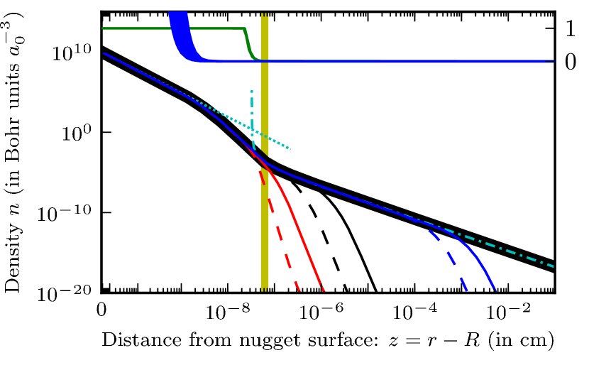
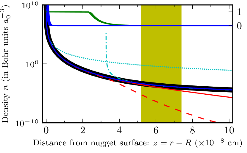
Figure 1: Density profile of antimatter nuggets (bottom plot is a zoom). The thick solid line is the one-dimensional approximation neglecting the curvature of the nugget. Six profiles are shown descending from this in pairs of thin solid and dashed curves. From left to right, each pair has fixed baryon charge $B=10^{20}$ (red), $10^{24}$ (black) and $10^{33}$ (blue) respectively. The solid curves represent nuclear density cores while the dashed curves represent 100 times nuclear density. The light shaded (yellow) regions correspond to the nonrelativistic Boltzmann regime where the Boltzmann approximation (10) (dash-dotted (cyan) line) is valid. Only the $B=10^{20}$ profiles visibly depart from the one-dimensional approximation in this regime. The two upper curves in the top plot use the scale on the right and are the annihilation rates $\Gamma_{Ps}$ (right (green) curve) and $\Gamma_{\text{dir}}$ (left (blue) curve) normalized to the saturated value $\Gamma_{Ps}(\mu=\infty)=4vq^{3}/(3\pi m^{2}\alpha^{2})$ (12). These curves comprise a range of cutoffs $q\sim m\alpha$ such the positronium annihilation rates (12) vary by 10%, and a range of incoming velocities $10^{-3}c<v<10^{-2}c$. The scaling of the abscissa in the upper figure is $\ln(z+z_{\textsc{ur}})$ where $z_{\textsc{ur}}\approx 5\times 10^{-11}$ so that the $T=0$ ultrarelativistic approximation (9) is linear (finely dotted (cyan) line). The abscissa are linearly spaced in the bottom figure.

Since we have the full density profiles, we fit $z_{\textrm{B}}$ here so that the this approximation matches the numerical solution at $n_{\textrm{B}}=(mT/2\pi)^{3/2}$, (a slightly better approximation than used in [5]).

All of our previous estimates about physical properties of the antimatter nuggets – emission of radiation, temperature etc. – have been based on these approximations using the region indicated in Fig. 1, it is clear that they work very well, as long as these regimes exist. The potential problem is that the nuggets could be highly charged or sufficiently small that the one-dimensional Boltzmann regime fails to exist with the density rapidly falling through the relevant density scales. We can see from the results in Fig. 1 that the nonrelativistic region exists for all but the smallest nuggets: As long as $B>10^{20}$ – as required by current detector constraints [4] – then the one-dimensional approximation suffices to calculate the physical properties.

The annihilation rates discussed in Sec. V have also been included in Fig. 1 to show that these effects only start once the densities have reached the atomic density scale, which is higher than the Boltzmann regime. Thus these results are also insensitive to the size of the nugget and the domain-wall approximation suffices. It is clear that one must have a proper characterization of the entire density profile from nonrelativistic through to ultrarelativistic regimes in order to properly calculate the emissions: one cannot use simple analytic forms.

We now discuss how charge equilibrium is established, and then apply our results to fix the relative normalization between the diffuse 1 – 20 MeV emissions and the 511 keV emissions from the core of our Galaxy. As we shall show, the relative normalization is now firmly rooted in conventional physics, and in agreement with the previous phenomenological estimate [6], providing another validation of our theory for dark matter.

IV.3 Nugget Charge Equilibrium

In order to determine the effective charge of the nuggets we must consider how equilibrium is obtained. For the matter nuggets, equilibrium is established through essentially static equilibrium with the surrounding ism plasma, however, for the antimatter nuggets, no such static equilibrium can be achieved. Instead, one must consider the dynamics of the following charge-exchange processes:

1. Deposition of charge via interaction and annihilation of neutral ism components (primarily neutral hydrogen).

2. Deposition of charge via interaction and annihilation of ionized ism components (electrons, protons, and ions).

3. Evaporation of positrons from the antinugget’s surface.

First we consider impinging neutral atoms or molecules with velocity $v_{\textsc{n},\textsc{ism}}\sim 10^{-3}c$. Even if the antinugget is charged, these are neutral and will still penetrate into the electrosphere. Here the electrons will annihilate or be ionized leaving a positively charge nucleus with energy $T_{\textsc{ism}}\sim\tfrac{1}{2}m_{\textsc{n}}v_{\textsc{n},\textsc{ism}}^{2}$. As the electrosphere consists of positrons, this charge cannot be screened, so the nucleus will accelerate to the core. At the core the nucleus either will penetrate and annihilate, resulting in the diffused x-ray emissions discussed in [4] and providing the heat to fuel the microwave emissions [5], or will bounce off of the surface due to the sharp quark-matter interface.

(0.8,0.35) i7 o7 label=$u$i7 label=$d$i6 label=$u$i5 label=$u$o7 label=$d$o6 label=$d$o5 label=$\bar{B}$i2 label=$\bar{B}$o2 fermion,right=0.2i7,o7 fermion,right=0.15i6,o6 phantom,right=0.1i5,o5 phantomo3,i3 fermiono2,i2 p[] p10vpath (__i5,__o5) p11vpath (__o3,__i3) p1vpath (__i7,__o7) p2vpath (__i6,__o6) p3subpath (0,0.4)*length(p10) of p10 .. subpath (0.6,1)*length(p11) of p11 p4subpath (0,0.4)*length(p11) of p11 .. subpath (0.6,1)*length(p10) of p10 p5vpath (__o2,__i2) fermionp3 fermionp4 fermionvpath (__o2,__i2) shifted ((0,0.1111h)) fermionvpath (__o2,__i2) shifted ((0,0.0555h)) fermionvpath (__o2,__i2) shifted ((0,-0.0555h)) fermionvpath (__o2,__i2) shifted ((0,-0.1111h)) curly_len1.5mm pair a[], k[]; a1 = (0.2,0.3); k1 = (1,2); a2 = (0.8,0.6); k2 = (1,2); a3 = (0.6,0.4); k3 = (3,4); a4 = (0.6,0.3); k4 = (4,3); a5 = (0.2,0.7); k5 = (4,4); a6 = (0.1,0.8); k6 = (3,5); a7 = (0.8,0.1); k7 = (2,5); for n = 1 upto 7: idraw ("gluon,fore=(0.5,,0.5,,0.5),width=0.1thin,rubout=15", point (xpart a[n])*length(p[xpart k[n]]) of p[xpart k[n]] – point (ypart a[n])*length(p[ypart k[n]]) of p[ypart k[n]]); endfor;

(0.8,0.35) i7 o7 label=$u$i7 label=$d$i6 label=$u$i5 label=$u$o7 label=$d$o6 label=$u$o5 label=$\bar{B}$i2 label=$\bar{B}$o2 fermion,right=0.2i7,o7 fermion,right=0.15i6,o6 fermion,right=0.1i5,o5 fermiono3,i3 fermiono2,i2 p[] p1vpath (__i7,__o7) p2vpath (__i6,__o6) p3vpath (__i5,__o5) p4vpath (__o3,__i3) p5vpath (__o2,__i2) fermionvpath (__o2,__i2) shifted ((0,0.1111h)) fermionvpath (__o2,__i2) shifted ((0,0.0555h)) fermionvpath (__o2,__i2) shifted ((0,-0.0555h)) fermionvpath (__o2,__i2) shifted ((0,-0.1111h)) curly_len1.5mm pair a[], k[]; a1 = (0.2,0.3); k1 = (1,2); a2 = (0.8,0.6); k2 = (1,2); a3 = (0.6,0.4); k3 = (3,4); a4 = (0.3,0.6); k4 = (3,4); a5 = (0.2,0.3); k5 = (4,5); a6 = (0.25,0.8); k6 = (3,5); a7 = (0.8,0.1); k7 = (2,5); for n = 1 upto 7: idraw ("gluon,fore=(0.5,,0.5,,0.5),width=0.1thin,rubout=15", point (xpart a[n])*length(p[xpart k[n]]) of p[xpart k[n]] – point (ypart a[n])*length(p[ypart k[n]]) of p[ypart k[n]]); endfor;

Figure 2: Charge-exchange process (top diagram): A charged incoming proton (upper left) exchanges an up quark $u$ for a down quark $d$ with the antimatter nugget $\bar{B}$, reflecting as a neutron (upper right). This is Zweig suppressed relative to the simple reflection process illustrated below, however, the neutron can escape from the system whereas the reflected proton will be trapped by the electric fields. This will enhance the overall rate of charge-exchange reactions because the proton will continue to react again and again until either the charge exchange occurs, or it eventually annihilates. In order to explain the relative intensities of the observed 511 keV and diffuse x-ray emissions from the core of our Galaxy [4], the ratio of the charge-exchange rate to the annihilation rate must be $f\sim 0.1$–$0.5$. To calculate this from microscopic physics, however, requires details of the nugget’s surface and equation of state that are not yet known. Perhaps some model-insensitive estimates could be made, which would provide a highly nontrivial test of our theory based on microscopic physics.

Note that, if the nuggets are sufficiently charged such that kinetic energy of the incoming nucleus at the point of ionization is smaller than the electrostatic energy,

$$T_{\textsc{ism}}\sim\tfrac{1}{2}m_{\textsc{n}}v_{\textsc{n},\textsc{ism}}^{2}\sim\text{eV}\ll\frac{eQ}{r}\sim\text{keV}\sim 10^{7}\text{ K},$$ (11)

then the charged nucleus will be unable to escape and will return to the core to either annihilate or undergo a charge-exchange reaction to become neutral, after which it may leave unimpeded by the electric field. For nuggets with $B\sim 10^{20}$, $10^{24}$, and $10^{33}$ respectively, this critical charge is $Q/e\gg 1$, $10^{2}$, and $10^{4}$ respectively. As shown in Table 1, the charge established through evaporation greatly exceeds this critical charge: The charged nucleus will not be able to escape the antinugget unless it undergoes a charge-exchange reaction (see Fig. 2).

For a single proton, such a charge-exchange reaction consists of an up quark being replaced by a down quark at the surface of the nugget, converting the proton to a neutron which can then escape. This process involves the exchange of a quark-antiquark pair and is a strong interaction process, but suppressed by the Zweig (ozi) rule. The overall ratio of charge-exchange to annihilation reactions is amplified by a finite probability of reflection from the core boundary: this results in multiple bounces before annihilation.

A better understanding of the details concerning the interaction between the proton and the quark-matter boundary is required to quantitatively predict the ratios of the rate of charge-exchange to the rate of annihilation and thus to confirm or rule out the suppression factor $f\sim 0.1$–$0.5$ required to explain the relative strengths of the observed 511 keV and diffuse $\sim 10$ keV x-ray emissions seen from the core of the Galaxy [4]. This requires an estimate of the rates of reflection, annihilation, and charge-exchange; the elasticity of collisions; and the energy loss through scattering.

We emphasize that the corresponding calculations do not require any new physics: everything is rooted firmly in qed and qcd. They do, however, require solving the many-body physics of the strong interaction including the incident nucleons and the quark antimatter interface (the phase of which may be quite complicated). A full calculation is thus very difficult, requiring insight into high-density qcd: estimates can probably be made using standard models of nuclear matter for the core, but are beyond the scope of the present paper.

In any case, the nucleus will certainly deposit its charge on the antinugget, and one may neglect the interactions with neutral ism components for the purpose of establishing charge neutrality.

Instead, we must consider the charged components. Using the same argument (11) one can see that the Coulomb barrier of the charged nuggets will be high enough to prevent electrons from reaching the electrosphere in all but the very hot ionized medium (vhim), which occupies only a small fraction of the ism in the core (see [53] for example). Protons however, will be able to reach the core to annihilate with a cross section $\sim 4\pi R^{2}$ (this is not substantially affected by the charge). Thus, positive charge can be deposited at a rate $\sim 4\pi R^{2}v_{\textsc{n}^{+},\textsc{ism}}n_{\textsc{n}^{+},\textsc{ism}}$ where $n_{\textsc{n}^{+},\textsc{ism}}$ is the density of the ionized components in the ism, which is typically $10^{-1}$ to $10^{-2}$ of the total density $n_{\textsc{ism}}\sim 1$ cm^-3

This rate of positive charge accumulation must match the evaporation rate of the positrons from the electrosphere (see Eq. (7)), giving the boundary conditions (8b), and the resulting charges summarized in Table 1. (These are consistent with the estimates in [24] and the universal upper bound [54].)

Note that the rate of evaporation is much less than the rate of proton annihilation and carries only $\sim 1$ eV of every per particle compared to the nearly 2 GeV of energy deposited. Thus, evaporation does not significantly cool the nuggets: the thermal radiation from the Boltzmann regime discussed in [5] dominates.

V Diffuse Galactic Emissions

Previous discussions of quark (anti)nugget dark matter considered the electrosphere in only two limiting cases: the inner high-density ultrarelativistic regime and the outer low-density Boltzmann regime. While this analysis was sufficient to qualitatively discuss the different components of the spectrum, it did not allow for their comparison in any level of detail. In particular, comparing the relative strengths of the 511 keV line emission (emitted entirely from the nonrelativistic regime) with that of the MeV continuum, (emitted from the relativistic regime) required introducing a phenomenological parameter $\chi\approx 0.1$ [6] to express the relative rates of direct annihilation to positronium formation. This parameter is sensitive to the density profile at all scales. Using the detailed numerical solutions of the previous section we can directly compute the relative intensities of the two emission mechanisms. Our calculation demonstrates that this value of $\chi$ is supported by a purely microscopic calculation rooted firmly in qed and well-understood many-body physics. The agreement between the calculated value of $\chi$ and the phenomenological value required to fit the observations provides another important and nontrivial test of our dark-matter proposal. In addition, using the same numerical solutions of the previous section, we compute the spectrum in the few MeV region which could not be calculated in [6] with only the ultrarelativistic approximation for the density profile.

V.1 Observations

V.1.1 The 511 keV Line

Spi/integral has detected a strong 511 keV signal from the Galactic bulge [55]. A spectral analysis shows this to be consistent with low-momentum $e^{+}e^{-}$ annihilation through a positronium intermediate state: About one quarter of positronium decays emit two 511 keV photons, while the remaining three-quarters will decay to a three photon state producing a continuum below 511 keV. Both emissions have been seen by spi/integral with the predicted ratios.

The 511 keV line is strongly correlated with the Galactic centre with roughly 80% of the observed flux coming from a circle of half angle 6^∘. There also appears to be a small asymmetry in the distribution oriented along the Galactic disk [56].

The measured flux from the Galactic bulge is found to be $\mathrm{d}\Phi/\mathrm{d}\Omega\simeq 0.025$ photons cm^-2 s^-1 sr^-1 [57]. After accounting for all known Galactic positronium sources the 511 keV line seems too strong to be explained by standard astrophysical processes. These processes, as we understand them, seem incapable of producing a sufficient number of low-momentum positrons. Several previous attempts have been made to account for this positron excess. Suggestions have included both modifications to the understood spectra of astrophysical objects or positrons which arise as a final state of some form of dark-matter annihilation. At this time there is no conclusive evidence for any of these proposals.

If we associate the observed 511 keV line with the annihilation of low momentum positrons in the electrosphere of an antiquark nugget, these properties are naturally explained. The strong peak at the Galactic centre and extension into the disk must arise because the intensity follows the distribution $\rho_{\textsc{v}}(\vec{\bm{r}})\rho_{\textsc{dm}}(\vec{\bm{r}})$ of visible and dark-matter densities. This profile is unique to dark-matter models in which the observed emission is due to matter–dark matter interactions and should be contrasted with the smoother $\sim\rho_{\textsc{dm}}^{2}(\vec{\bm{r}})$ profile for proposals based on self-annihilating dark-matter particles, or the $\sim\rho_{\textsc{dm}}(\vec{\bm{r}})$ profile for decaying dark-matter proposals. The distribution $\rho_{\textsc{v}}(\vec{\bm{r}})\rho_{\textsc{dm}}(\vec{\bm{r}})$ obviously implies that the predicted emission will be asymmetric, with extension into the disk from the Galactic center as it tracks the visible matter. There appears to be evidence for an asymmetry of this form [56]. In our proposal, no synchrotron emission will occur as the positrons are simply an integral part of the nuggets rather than being produced at high energies with only the low-energy components exposed for emission. Contrast this with many other dark matter based proposals where the relatively high-energy positrons produced from decaying or annihilating dark-matter particles produce strong synchrotron emission. These emissions are typically in conflict with the strong observational constraints [27].

V.1.2 Diffuse MeV scale emission

The other component of the Galactic spectrum we discuss here is the diffuse continuum emission in the 1 – 30 MeV range observed by comptelcrgo. The interpretation of the spectrum in this range is more complicated than that of the 511 keV line as several different astrophysical processes contribute.

The conventional explanation of these diffuse emissions is that of gamma rays produced by the scattering of cosmic rays off of the interstellar medium, and while detailed studies of cosmic ray processes provide a good fit to the observational data over a wide energy range (from 20 MeV up to 100 GeV), the predicted spectrum falls short of observations by roughly a factor of 2 in the 1 – 20 MeV range [58].

Background subtraction is difficult, however, and especially obscures the spatial distribution of the MeV excess. However, the excess seems to be confined to the inner Galaxy ($l=330^{\circ}$ – $30^{\circ},|b|=0^{\circ}$ – $5^{\circ}$), [58] with a negligible excess from outside of the Galactic centre.

V.1.3 Comparison

As our model predicts both of these components to have a common source, a comparison of these emissions provides a stringent tests of the theory. In particular, the morphologies, spectra, and relative intensities of both emissions must be strongly related.

The inferred spatial distribution of these emissions is consistent: both are concentrated in the core of the Galaxy. Unfortunately, this is not a very stringent test due to the poor spatial resolutions of the present observations. The prediction remains firm: If the morphology of the observations can be improved, then a full subtraction of known astrophysical sources should yield a diffuse MeV continuum with spatial morphology identical to that of the 511 keV.

Present observations, however, do allow us to test the intensity and spectrum predicted by the quark nugget dark-matter model. The model predicts the intensity to be proportional to the 511 keV flux with calculable coefficient of proportionality. Therefore, the integral data may be used to fix the total diffuse emission flux, removing the uncertainties associated with the line of sight averaging which is the same for both emissions.

The resulting spectrum and intensity were previously discussed in [30] and [6], but the 511 keV line emission was estimated using the low-density Boltzmann approximation, while the MeV emissions were estimated using the high-density ultrarelativistic approximation. The proportionality factor linking these two was treated as a phenomenological parameter, $\chi$, which required a value of $\chi\approx 0.1$ [6] in order to explain the observations. Here, equipped with a complete density profile, we calculate the value of this parameter from first principles showing that it is indeed consistent with the observations, providing yet another highly nontrivial verification of the quark antimatter nugget dark-matter proposal.

V.2 Annihilation rates

As incident electrons enter the electrosphere of positrons, the dominant annihilation process is through positronium formation with the subsequent annihilation producing the 511 keV emission. As the remaining electrons penetrate more deeply, they will encounter a higher density of more energetic positrons: Direct annihilation eventually becomes the dominant process. The maximum photon energy, $\sim 10$ MeV, is determined by the Fermi energy of the electrosphere at the deepest depth of electron penetration. We stress that this scale is not introduced in order to explain the comptel/crgo gamma-ray excess: Our model necessarily produces a strong emission signature at precisely this energy.

In the following section we integrate the rates for these two processes over the complete density profile, allowing us to predict the relative intensities and spectral properties of the emissions.

V.2.1 Positronium Formation

In principle, we only need to know the $e^{+}e^{-}$ annihilation cross section at all centre of mass momenta. At high energies, this is perturbative and one can use the standard qed result for direct $e^{+}e^{-}\rightarrow 2\gamma$ emission. At low energies, however, one encounters a strong resonance due to the presence of a positronium state the greatly enhances the emission. This resonance renders a perturbative treatment invalid and must be dealt with specially, thus we consider these as two separate processes. Our presentation here will be abbreviated: details may be found in [30].

While the exact positronium formation rate – summed over all excited states – is not well established, it is clear that the rate will fall off rapidly as the centre of mass momentum moves away from resonance. A simple estimate suggests that for momenta $p>m\alpha$ the formation rate falls as $\sim p^{-4}$. To estimate the rate, we thus make a cutoff at $q\approx m\alpha$ as the upper limit for positronium formation: for large center of mass momenta we use the perturbative direct-annihilation approximation. The scale here is set by the Bohr radius $a_{b}=2(m\alpha)^{-1}$ for the positronium bound state: If a low-momentum $e^{+}e^{-}$ pair pass within this distance, then the probability of forming a bound state becomes large, with a natural cross section $\sigma_{Ps}\sim\pi a_{b}^{2}$. The corresponding rate is

$$\Gamma_{Ps}=\int_{p\lesssim q}\!\!\!\!v\sigma_{Ps}n(p)\frac{\mathrm{d}^{3}{p}}{(2\pi)^{3}}\sim\frac{4v}{m^{2}\alpha^{2}}\begin{cases}n(p)\pi&p_{F}\lesssim q\\ \frac{q^{3}}{3\pi}&p_{F}\gtrsim q.\end{cases}$$ (12)

where $n(p)$ is the momentum distribution of the positrons in the electrosphere, and $v\sim\alpha$ is the incoming electron velocity. The second expression represents the two limits (valid at low temperature): a) of low density when the Fermi momentum $p_{F}\lesssim q$ and all states participate, resulting in a factor of the total density $n$, and b) of high density where the integral is saturated by $q^{3}/3\pi^{2}\approx(m\alpha)^{3}/3\pi^{2}$.

As discussed in Sec. IV.3, and in more detail in Appendix B, electrons will be able to penetrate the charged antimatter nuggets in spite of the strong electric field. Initially the electrons are bound in neutral atoms. Once ionized, the density is sufficiently high that the charge is efficiently screened with a Debye screening length $\lambda_{D}$ that is much smaller than the typical de Broglie wavelength $\lambda=\hbar/p$ of electrons. Thus, the electric fields – although quite strong in the nugget’s electrosphere – will not appreciably effect the motion. The binding of electrons in neutral atoms complicates the analysis slightly, but the binding energy – on the eV scale – will not significantly alter the qualitative nature of our estimates. For a precision test of the emission properties, this will need to be accounted for. Here we include bands comprising $\pm 10\%$ relative variation in the overall positronium annihilation rate to show the sensitivity to this uncertainty.

V.2.2 Direct-annihilation Rates

While positronium formation is strongly favoured at low densities due to its resonance nature, deep within the electrosphere the rapidly growing density of states at large momentum values result in a cross section characterized by the perturbative direct-annihilation process. Conceptually one can imagine an incident Galactic electron first moving through a Fermi gas of positrons with roughly atomic density with a relatively large probability of annihilation through positronium to 511 keV photons. A small fraction survive to penetrate to the inner high0density region where direct annihilation dominates. The surviving electrons then annihilate with a high-energy positron near to the inner quark-matter surface releasing high-energy photons. The spectrum of these annihilation events will be a broad continuum with an upper cutoff at an energy scale set by the Fermi energy of the positron gas at the maximum penetration depth of the electrons. The spectral density for direct $e^{+}e^{-}$ annihilation at a given chemical potential was calculated in [6]:

$$\frac{\mathrm{d}{I(\omega,\mu)}}{\mathrm{d}{}\omega\mathrm{d}{t}} =\int\mathrm{d}{n_{p}(\mu)}\;v_{p}(\mu)\frac{\mathrm{d}\sigma(p,\omega)}{\mathrm{d}{\omega}}$$ (13)

$$=\int\frac{\mathrm{d}^{3}{p}}{(2\pi)^{3}}\frac{2}{1+\mathrm{e}^{(\mu-E_{p})/T}}\frac{p}{E_{p}}\frac{\mathrm{d}\sigma(p,\omega)}{\mathrm{d}{\omega}}$$

$$\frac{\mathrm{d}\sigma(p,\omega)}{\mathrm{d}{\omega}} =\frac{\pi\alpha^{2}}{mp^{2}}\Biggl{[}\frac{-(3m+E_{p})(m+E_{p})}{(m+E_{p}-\omega)^{2}}-2$$ (14)

$$+\frac{\frac{1}{\omega}(3m+E_{p})(m+E_{p})^{2}-(\frac{m}{\omega})^{2}(m+E_{p})^{2}}{(m+E_{p}-\omega)^{2}}\Biggr{]},$$

where $E_{p}=\sqrt{p^{2}+m^{2}}$ is the energy of the positron in the rest frame of the incident (slow-moving) electron and $\omega$ is the energy of the produced photons. The annihilation rate at a given density, $\Gamma_{\text{dir}}(n_{\mu})$, is obtained by integrating over allowed final state photon momentum. This was previously done in the $T\rightarrow$ 0 limit where the integral may be evaluated analytically, at nonzero temperatures the rate must be evaluated numerically.

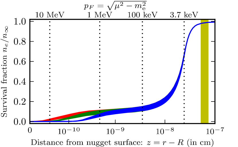
Figure 3: Electron survival fraction, $n_{e}(r)/n_{\infty}$ (16), of an incoming electron with velocities $v=0.01c$ [leftmost light gray (red) band], $v=0.005c$ [middle (green) band] and $v=0.001c$ [rightmost dark gray (blue) band] from left to right, respectively. The thickness of the bands includes a $\pm 10\%$ variation in the positronium annihilation rate (12). The local Fermi momentum $p_{F}$ is shown along the top and with vertical dotted lines including the cutoff scale $q\approx 3.7$ keV from (12). The yellow shaded Boltzmann region and the abscissa scaling are the same as in the top of Fig. 1. Note that annihilation happens well within the electrosphere, so the finite size of the nugget is irrelevant.

V.3 Spectrum and Branching Fraction

To determine the full annihilation spectrum we first determine the fraction of incident electrons that can penetrate to a given radius $r$ in the electrosphere (see Fig. 3. We then integrate the emissions over all regions.

Consider an incident beam of electrons with density $n_{\infty}$ and velocity $v$. As they enter the electrosphere of positrons, the electrons will annihilate. The survival fraction $n_{e}(r)/n_{\infty}$ will thus decrease with a rate proportional to $\Gamma(r)=\Gamma_{Ps}(r)+\Gamma_{\text{dir}}(r)$ which depends crucially on the local density profile $n[\mu(r)]$ calculated in Sec. IV.2:

$$\frac{\mathrm{d}{n_{e}}(r)}{\mathrm{d}{t}}=v^{-1}\frac{\mathrm{d}{n_{e}}(r)}{\mathrm{d}{r}}=-\Gamma(r)v^{-1}n_{e}(r).$$ (15)

Integrating (15), we obtain the survival fraction:

$$\frac{n_{e}(r)}{n_{\infty}}=\exp\left(-\int_{r}^{\infty}\mathrm{d}{r}\;v^{-1}\Gamma(r)\right).$$ (16)

This is shown in Fig. 3. One can clearly see that in the outer electrosphere, positronium formation – independent of $v$ – dominates the annihilation. Once the density is sufficiently high ($p_{F}\gtrsim 1$ MeV), the direct-annihilation process dominates, introducing a dependence on the velocity $v$ of the incident particle.

The initial velocity $v\sim 10^{-3}c$ is determined by the local relative velocity of the nuggets with the surrounding ism. This will depend on the temperature of the ism, but the positronium annihilation rate is insensitive to this. As we mentioned previously, most of the electrons in the interstellar medium are bound in neutral atoms, either as neutral hydrogen HI, or in molecular form H₂. (The ionized hydrogen HII represents a very small mass fraction of interstellar medium.) These neutral atoms and molecules will have no difficulty entering the electrosphere.

The remaining bound electrons that do not annihilate through positronium will ionize once they reach denser regions, and will acquire a new velocity set by a combination of the initial velocity $v\sim 10^{-3}c$ and the atomic velocity $v\sim\alpha\sim 10^{-2}c$ imparted to the electrons as they are ionized from the neutral atoms: The latter will typically dominate the velocity scale. This only occurs in sufficiently dense regions where the Debye screening discussed in Appendix B becomes efficient. Hence, the electric fields will not significantly alter the motion of the electrons after ionization. The direct-annihilation process depends on the final velocity $v$; as the dominant contribution comes from ionization, this will remain relatively insensitive to the ism. During ionization, some fraction (roughly half) of the electrons will move away from the core, but a significant portion will travel with this velocity $v$ toward the denser regions.

Two other features of Fig. 3 should be noted. First is the value of the survival fraction $\chi\sim 0.1$ at which direct annihilation dominates [see Eq. 19]. This is the value that was postulated phenomenologically in [6] in order to explain the relative intensities of the 511 keV and direct-annihilation spectra. Here this value results naturally from a microscopic calculation in a highly nontrivial manner that depends on the structure of the density profile at all scales up to $p_{F}=1$ MeV. Second is the rapid increase in density near the core quickly extinguishes any remaining electrons. As such, even if the chemical potential at the surface is larger – $\mu_{R}\sim 100$ MeV or so – virtually no Galactic electrons penetrate deeply enough to annihilate at these energies. For nonrelativistic electrons the maximum energy scale for emission is quite generally set at the $\sim$ 20 MeV scale, depending slightly on $v$.

Having established the survival fraction as a function of height it is now possible to work out the spectral density that will arise from the $e^{+}e^{-}$ annihilations. At a given height we can express the number of annihilations through a particular channel as,

$$\frac{\mathrm{d}{n}}{\mathrm{d}{r}}=n_{e}(r)v^{-1}\Gamma(r).$$ (17)

Integrating this expression over all heights will then give the total fraction of annihilation events proceeding via positronium $f_{511}$, and via direct annihilation $f_{\text{MeV}}$. (The numerical values are given for $q=m\alpha$ and are quite insensitive to $v$.)

$$f_{511} =\int_{R}^{\infty}\!\!\!\mathrm{d}{r}\;\frac{n_{e}(r)}{n_{\infty}}v^{-1}\Gamma_{Ps}(r)\approx 0.9,$$ (18a)

$$f_{\text{MeV}} =\int_{R}^{\infty}\mathrm{d}{r}\;\frac{n_{e}(r)}{n_{\infty}}v^{-1}\Gamma_{\text{dir}}(r)\approx 0.1.$$ (18b)

Note that in both cases, the overall normalization depends only on the total rate of electron collisions with dark matter through $vn_{\infty}$. As such, the ratio of 511 keV photons to MeV continuum emission is independent of the relative densities (though it will show some dependence on the local electron velocity distribution). Numerically, with a $\pm 10\%$ variation in the positronium annihilation rate, we find

$$\chi=\frac{f_{\text{MeV}}}{f_{511}}\approx 0.05-0.2,$$ (19)

which is quite insensitive to the velocity $v$. This ratio was introduced as a purely phenomenological parameter in [6] to explain the observations. Here we have calculated from purely microscopic considerations that, for a wide range of nugget parameters, the required value $\chi\sim 0.1$ [6] arises quite naturally.

We now have everything needed to compute the spectral density of the MeV continuum. The spectral density at a fixed chemical potential is given by Eq. (13): this must now be averaged along the trajectory of the incoming electron weighted by the survival fraction (16) and the time spent in the given region of the trajectory (set by the inverse velocity $v^{-1}$):

$$\frac{\mathrm{d}{I_{\text{total}}}}{\mathrm{d}{\omega}}=\int_{R}^{\infty}\mathrm{d}{r}\;v^{-1}\frac{n_{e}(r)}{n_{\infty}}\frac{\mathrm{d}{I(\mu(r))}}{\mathrm{d}{\omega}\;\mathrm{d}{t}}.$$ (20)

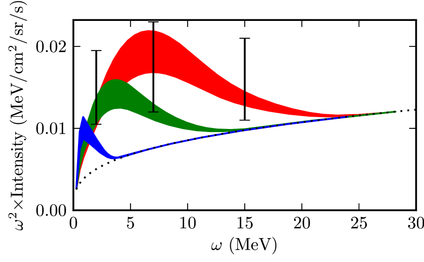
Figure 4: Spectral density (scaled by $\omega^{2}$ to compare with [58] of photons emitted by an electron annihilating on antiquark nuggets with incoming velocities $v=0.01c$ [uppermost (red) band], $v=0.005c$ [middle (green) band] and $v=0.001c$ [lowest (blue) band to the lower left] from right to left, respectively, including the cosmic ray background determined in [58] (dotted line). The thickness of the bands includes a $\pm 10\%$ variation in the positronium annihilation rate (12). The overall normalization is fixed to the observationally unrelated 511 keV line as discussed below (21). The three error bars are the comptel data points. Note: This spectrum should still be interpreted as a qualitative effect - a detailed calculation of the ionization and hence distribution of the velocity $v$ must be performed to yield a quantitative prediction. The general structure and magnitude, however, can be trusted as these depend on the overall density profile which we have carefully modeled. (Compare with Fig. 5, for example, which uses only the ultrarelativistic density profile: The resulting intensity is 2 orders of magnitude too large.)

The resulting spectrum is shown in Fig. 4 and is sensitive to both the incoming velocity $v$ (which will depend on the local environment of the antimatter nugget) and the overall normalization of the positronium annihilation rate (12). (The latter is fixed in principle, but requires a difficult in-medium calculation to determine precisely.) These two parameters are rather orthogonal. The velocity $v$ determines the maximum depth of penetration, and hence the maximum energy of the emitted photons (as set by the highest chemical potential at the annihilation point): If the electron velocity is relatively low ($v<100$ km/s $\approx 0.0003c$), almost all annihilations happen immediately and the MeV continuum will fall rapidly beyond 5 MeV. As the velocity increases the electrons are able to penetrate deeper toward the quark surface and annihilate with larger energies. In contrast, the details of the positronium annihilation do not alter the spectral shape, but do alter the overall normalization.

As already mentioned earlier, the parameter $\chi\sim 0.1$ is calculated here from purely microscopic physics. Therefore, it provides highly nontrivial verification of the entire proposal. Also, the profile function from the previous section is computed at all scales, allowing us to calculate the photon spectrum down to, and below, the electron mass. This calculation could not be performed in the previous analysis [6] with only the ultrarelativistic expression.

We stress here that the result shown in Fig. 4 exhibits several nontrivial features arising from very general characteristics of the proposed emission model. The wide range of positron energies within the electrosphere implies a broad emission profile with a width $\Delta\omega\simeq 5$ – $10$ MeV. The initial growth of emission strength with $\omega$ is due to the increasing density of states as a function of depth. Above $\sim 10$ MeV, the emission becomes suppressed by the inability of Galactic electrons to penetrate to depths where the positrons have this energy. While the exact details may vary with parameters, such as the local electron velocity and precise rate of positronium formation, the general spectral features are inescapable consequences of our model, allowing it to be tested by future, more precise, observations.

V.4 Normalization to the 511 keV line

To obtain the observed spectrum, one needs to average (20) along the line of site over the varying matter and dark-matter density and velocity distributions. Neither of these is known very well, so to check whether or not the prediction is significant, we fix the average rate of electron annihilation with the observed 511 keV line which our model predicts to be produced by the same process. As the intensity of the 511 keV line (resulting from the two-photon decay of positronium in the ¹S₀ state) has been measured by spi/integral along the line of sight toward the core of the Galaxy (see [59] for a review), we can use this to fix the normalization of the MeV spectrum along the same line of sight. The total intensity is given in terms of Eq. (18a):

$$\frac{\mathrm{d}{\Phi}}{\mathrm{d}{\Omega}}=\frac{C}{4}f_{511}\sim\;0.025\;\frac{\text{photons}}{\text{cm}^{2}\text{~{}s}\text{~{}sr}}\;,$$ (21)

where the factor of $4$ accounts for the three-quarters of the annihilation events that decay via the ³S₁ channel (also measured, but not included in the line emission). This fixes the normalization constant $C\approx 0.11$ events cm^-2 s^-1 sr^-1. The predicted contribution to the MeV continuum must have the same morphology and, thus, an integrated intensity along the same line of sight must have the same normalization factor. This normalization has been used in Fig. 4 to compare the predicted spectrum with the unaccounted for excess emission detected by comptel ([58]).

The exact shape of the spectrum will be an average of the components shown over the velocity distribution of the incident matter. Our process of normalization is unable to remove this ambiguity because the predicted 511 keV spectral properties are insensitive to this. It is evident, however, that MeV emission from dark-matter nuggets could easily provide a substantial contribution to the observed MeV excess. Note also, that the excess emission can extend only to 20 MeV or so. This is completely consistent with the more sophisticated background estimates discussed in [60] which can fit almost all aspects of the observed spectrum except the excess between 1 and 30 MeV predicted by our proposal.

VI Conclusion

Solving the relativistic Thomas-Fermi equations, we determined the charge and structure of the positron electrosphere of quark antimatter nuggets that we postulate could comprise the missing dark-matter in our Universe. We found the structure of the electrosphere to be insensitive to the size of the nuggets, as long as they are large enough to be consistent with current terrestrial based detector limits, and hence, can make unambiguous predictions about electron annihilation processes.

To test the dark-matter postulate further, we used the structure of this electrosphere to calculate the annihilation spectrum for incident electronic matter. The model predicts two distinct components: a 511 keV emission line from decay through a positronium intermediate and an MeV continuum emission from direct-annihilation processes deep within the electrosphere. By fixing the general normalization to the measured 511 keV line intensity seen from the core of the Galaxy, our model makes a definite prediction about the intensity and spectrum of the MeV continuum spectrum without any additional adjustable model parameters: Our predictions are based on well-established physics.

As discussed in [36], a difficulty with most other dark-matter explanations for the 511 keV emission is to explain the large $\sim$100% observed positronium fraction – positrons produced in hot regions of the Galaxy would produce a much smaller fraction. Our model naturally predicts this observed ratio everywhere.

A priori, there is no reason to expect that the predicted MeV spectrum should correspond to observations: typically two uncorrelated emissions are separated by many orders of magnitude. We find that the phenomenological parameter $\chi$ (19) required to explain the relative normalization of MeV emissions arises naturally from our microscopic calculation. This is highly nontrivial because it requires a delicate balance between the two annihilation processes from the semirelativistic region of densities that is sensitive to the semirelativistic self-consistent structure of the electrosphere outside the range of validity of the analytic ultrarelativistic and nonrelativistic regimes. (See Fig. 1 and 3).

If the predicted emission were several orders of magnitude too large, the observations would have ruled out our proposal. If the predicted emissions were too small, the proposal would not have been ruled out, but would have been much less interesting. Instead, we are left with the intriguing possibility that both the 511 keV spectrum and much of the MeV continuum emission arise from the annihilation of electrons on dark-antimatter nuggets. While not a smoking gun – at least until the density and velocity distributions of matter and dark-matter are much better understood – this provides another highly nontrivial test of the proposal that, a priori, could have ruled it out.

Both the formal calculations and the resulting structure presented here – spanning density regimes from ultrarelativistic to nonrelativistic – are similar to those relevant to electrospheres surrounding strange-quark stars should they exist. Therefore, our results may prove useful for studying quark star physics. In particular, problems such as bremsstrahlung emission from quark stars originally analyzed in [61] (and corrected in [62]) that uses only ultrarelativistic profile functions. The results of this work can be used to generalize the corresponding analysis for the entire range of allowed temperatures and chemical potentials. Another problem which can be analyzed using the results of the present work is the study of the emission of energetic electrons produced from the interior of quark stars. As advocated in [63], these electrons may be responsible for neutron star kicks, helical and toroidal magnetic fields, and other important properties that are observed in a number of pulsars, but are presently unexplained.

Finally, we would like to emphasize that this mechanism demonstrates that dark matter may arise from within the standard model at the qcd scale, and that exotic new physics is not required. Indeed, this is naturally suggested by the “cosmic coincidence” of almost equal amounts of dark and visible contributions to the total density $\Omega_{\text{tot}}=1.011(12)$ of our Universe [22]:

$$\Omega_{\text{dark-energy}}:\Omega_{\text{dark-matter}}:\Omega_{\text{visible}}\approx 17:5:1.$$

The dominant baryon contribution to the visible portion $\Omega_{\text{visible}}\approx\Omega_{B}$ has an obvious relation to qcd through the nucleon mass $m_{\textsc{n}}\propto\Lambda_{\textsc{qcd}}$ (the actual quark masses arising from the Higgs mechanism contribute only a small fraction to $m_{\textsc{n}}$). Thus, a qcd origin for the dark components would provide a natural solution to the extraordinary “fine-tuning” problem typically required by exotic high-energy physics proposals. Our proposal here solves the matter portion of this coincidence. For a proposal addressing the energy coincidence we refer the reader to [64, *Urban:2009yg] and references therein.

Note in proof:

While this paper was in preparation, a review [69] was submitted which mentions the mechanism discussed here, but dismisses it based on the arguments of [51]. This work makes it clear that the assumptions used in [51] are invalid (see footnote 7) and addresses the issues raised therein. The arguments of [51] were previously addressed in [5] (at the end of appendix 1) where it was emphasized that [51] incorrectly applies a relativistic formula to the non-relativistic regime.

Appendix A Density Functional Theory

We start with a Density Functional Theory (dft) formulated in terms of the thermodynamic potential:

$$\Omega=\sum_{i}2f_{i}\int\mathrm{d}^{3}\vec{\bm{r}}\;\psi^{\dagger}_{i}(\vec{\bm{r}})(\epsilon_{-i\hbar\vec{\bm{\nabla}}}-\mu)\psi_{i}(\vec{\bm{r}})+\\ +\int\mathrm{d}^{3}\vec{\bm{r}}V_{\text{ext}}(\vec{\bm{r}})n(\vec{\bm{r}})+\int\mathrm{d}^{3}\vec{\bm{r}}\;\varepsilon_{\text{xc}}\Bigl{[}n(\vec{\bm{r}})\Bigr{]}n(\vec{\bm{r}})+\\ +\frac{4\pi e^{2}}{2}\int\mathrm{d}^{3}{\vec{\bm{r}}}\;\mathrm{d}^{3}{\vec{\bm{r}}^{\prime}}\;\frac{n(\vec{\bm{r}})n(\vec{\bm{r}}^{\prime})}{\lVert{\vec{\bm{r}}-\vec{\bm{r}}^{\prime}}\rVert}-T\sum_{i}f_{i}\ln f_{i},$$ (22a)

where $$\epsilon_{p}=\sqrt{p^{2}+m^{2}} \varepsilon_{\text{xc}}(n)$$ is the relativistic energy of the electrons, is the exchange energy. The density is

$$n(\vec{\bm{r}})=2\sum_{i}f_{i}\psi_{i}^{\dagger}(\vec{\bm{r}})\psi_{i}(\vec{\bm{r}}),$$ (22b)

where we have explicitly included the spin degeneracy, and used relativistic units where $$\hbar=c=1 e^{2}=\alpha$$ and .

We vary the potential with respect to the occupation numbers $f_{i}$ and the wave functions $\psi_{i}$ subject to the constraints that the wave functions be normalized,

$$\int\mathrm{d}^{3}\vec{\bm{r}}\;\psi_{i}^{\dagger}(\vec{\bm{r}})\psi_{j}(\vec{\bm{r}})=\delta_{ij},$$ (22c)

and that the occupation numbers satisfy Fermi-Dirac statistics. This yields the Kohn-Sham equations for the electronic wave functions:

$$\Bigl{[}\epsilon_{(-i\hbar\vec{\bm{\nabla}})}-\mu+V_{\text{eff}}(\vec{\bm{r}})\Bigr{]}\psi_{i}(\vec{\bm{r}}) =E_{i}\psi_{i}(\vec{\bm{r}}),$$

$$f_{i} =\frac{1}{1+\mathrm{e}^{E_{i}/T}}.$$

where (we take $e$ to be positive here)

$$V_{\text{eff}}(\vec{\bm{r}})=e\phi(\vec{\bm{r}})+V_{\text{ext}}(\vec{\bm{r}})+\varepsilon_{\text{xc}}[n(\vec{\bm{r}})]+n(\vec{\bm{r}})\varepsilon_{\text{xc}}^{\prime}[n(\vec{\bm{r}})]$$

and

$$\phi(\vec{\bm{r}})=4\pi e\int\mathrm{d}^{3}\vec{\bm{r}}^{\prime}\frac{n(\vec{\bm{r}}+\vec{\bm{r}}^{\prime})}{\lVert{\vec{\bm{r}}}\rVert}$$

is the electrostatic potential obeying Poisson’s equation,

$$\nabla^{2}\phi(\vec{\bm{r}})=-4\pi en(\vec{\bm{r}}).$$

A.1 Thomas-Fermi Approximation.

If the effective potential $$V_{\text{eff}}(\vec{\bm{r}}) i\equiv k \psi_{k}\propto\mathrm{e}^{ikr}$$ varies sufficiently slowly, then it is a good approximation to replace it locally with a constant potential. The Kohn-Sham equations thus become diagonal in momentum space, , and may be explicitly solved:

$$E_{\vec{\bm{k}}}(\vec{\bm{r}})=\epsilon_{\vec{\bm{k}}}-\mu+V_{\text{eff}}(\vec{\bm{r}}),$$

$$n(\vec{\bm{r}})=2\int\frac{\mathrm{d}^{3}\vec{\bm{k}}}{(2\pi)^{3}}\left(\frac{1}{1+\mathrm{e}^{E_{\vec{\bm{k}}}(\vec{\bm{r}})/T}}-\frac{1}{1+\mathrm{e}^{-E_{\vec{\bm{k}}}(\vec{\bm{r}})/T}}\right),$$

where we have also explicitly included the contribution from the antiparticles. We piece these homogeneous solutions together at each point $$\vec{\bm{r}}$$ and find the self-consistent solution that satisfies Poisson’s equation. This approximation is a relativistic generalization of the Thomas-Fermi approximation.

In principle, the dft method is exact [66], however, the correct form for $\varepsilon_{\text{xc}}$ is not known and could be extremely complicated. Various successful approximations exist but for our purposes we may simply neglect this. The weak electromagnetic coupling constant $\alpha\sim 1/137$ and Pauli exclusion principle keep the electrons sufficiently dilute that the many-body correlation effects can be neglected until the density is high in the sense that $\alpha^{2}n\sim\alpha^{2}\mu^{3}/3\pi^{3}\gtrsim m^{3}$, which corresponds to $\mu\gtrsim 50$ MeV.

Near the nugget core, many-body correlations may become quantitatively important. For example, the effective mass of the electrons in the gas is increased by about $20\%$ when $\mu\approx 25$ MeV and doubles when $\mu\approx 100$ MeV (see, for example, [67]). These effects, however, will not change the qualitative structure, and can be quite easily taken into account if higher accuracy is required. We also note that, formally, the Thomas-Fermi approximation is only valid for sufficiently high densities. However, it gives correct energies within factors of order unity for small nuclei [50] and is known to work substantially better for large nuclei [68]. As long as we do not attempt to use it in the extremely low-density tails, it should give an accurate description.

A.2 Analytic Solutions

There are several analytic solutions available if we consider the one-dimensional approximation, neglecting the curvature term $2\mu^{\prime}(r)/r$ in (5), which is valid close to the nugget where $z=r-R\ll R$, the distance from the nugget core, is less than the radius of the nugget.

A.2.1 Ultrarelativistic Regime

The first is the ultrarelativistic approximation where $\mu$ and/or $T$ are much larger than $m$ and the limit $m\rightarrow 0$ can be taken. In this case, we may explicitly evaluate (see also [46, 47, 48]),

$$n[\mu,T]_{m\ll\mu,T}=\frac{\mu^{3}}{3\pi^{2}}+\frac{\mu T^{2}}{3}.$$ (26)

In the domain-wall approximation, this admits an exact solution with a typical length scale of $z_{\textsc{ur}}$:

$$\mu(z,T)=\frac{T\pi\sqrt{2}}{\sinh\left[2T\sqrt{\frac{\alpha\pi}{3}}(z+z_{T})\right]},$$ (27)

$$z_{\textsc{ur}}=\frac{1}{2T}\sqrt{\frac{3}{\alpha\pi}}\sinh^{-1}\left(\frac{T\pi\sqrt{2}}{\mu_{R}}\right).$$ (28)

In our case, $T\sim 1\text{ eV }\ll m$ so we can also take the $T\rightarrow 0$ limit to obtain (9):

$$n_{\textsc{ur}}(z) \approx\frac{\mu_{R}^{3}}{3\pi^{2}(1+z/z_{\textsc{ur}})^{3}}, z_{\textsc{ur}} \approx\mu_{R}^{-1}\sqrt{\frac{3\pi}{2\alpha}}.$$ (29)

This solution persists until $\mu\approx m$, which occurs at a distance

$$z_{\textrm{B}}\approx z_{\textsc{ur}}\left(\frac{\mu_{R}}{m}-1\right)\approx m^{-1}\sqrt{\frac{3\pi}{2\alpha}}.$$ (30)

A.2.2 Boltzmann Regime

Once the chemical potential is small enough that $\mathrm{e}^{\mu/T}\ll\mathrm{e}^{m/T}$, we may neglect the degeneracy in the system, and write

$$\left.n[\mu]\right|_{\exp(\mu/T)\ll\exp(m/T)}\approx n_{0}\mathrm{e}^{\mu/T}.$$ (31)

This occurs for a density of about

$$n_{\textrm{B}}\approx\left(\frac{mT}{2\pi}\right)^{3/2}$$ (32)

and lower. If the one-dimensional approximation is still valid, then another analytic solution may be found:

$$n(z) =\frac{n_{\textrm{B}}}{\left(1+\frac{z-z_{\textrm{B}}}{z_{\alpha}}\right)^{2}}, z_{\alpha} =\sqrt{\frac{T}{2\pi\alpha n_{\textrm{B}}}}$$ (33)

from which we obtained (10). The shift $z_{\textrm{B}}$ must be determined from the numerical profile at the point where $n(z_{\textrm{B}})=n_{\textrm{B}}$. Note that $z_{\alpha}\ll z_{\textrm{B}}$, so this regime is valid and persists until $z\sim 0.1R$, at which point the one-dimensional approximation breaks down. It is in this Boltzmann regime where most of the important radiative processes take place [5].

A.3 Numerical Solutions

The main technical challenge in finding the numerical solution is to deal effectively with the large range of scales: $T\sim 1\text{ eV}\ll m\sim 500\text{ keV}\ll\mu_{R}\sim 25\text{ MeV}$. For example, the density distribution (4b) is prone to round-off error, but the integral can easily be rearranged to give a form that is manifestly positive:

$$n[\mu]=\frac{1}{\pi^{2}}\int_{0}^{\infty}\!\!\!\!\!\mathrm{d}{p}\;\frac{p^{2}\sinh\left(\frac{\mu}{T}\right)}{\cosh\left(\frac{\sqrt{p^{2}+m^{2}}}{T}\right)+\cosh\left(\frac{\mu}{T}\right)}.$$ (34)

The derivative may also be safely computed. Let

$$A =\frac{\sqrt{p^{2}+m^{2}}}{T}, B =\frac{\mu}{T},$$ (35)

to simplify the expressions. These can each be computed without any round-off error. The first derivative presents no further difficulties:

$$\dot{n}[\mu]=\frac{1}{T\pi^{2}}\int_{0}^{\infty}\!\!\!\!\!\mathrm{d}{p}\;p^{2}\frac{1+\cosh{A}\cosh{B}}{\left(\cosh{A}+\cosh{B}\right)^{2}}.$$ (36)

The differential equation is numerically simplified if we change variables to logarithmic quantities. We would also like to capture the relevant physical characteristics of the solution, known from the asymptotic regimes. Close to the nugget, we have $\mu=\mu_{R}/(1+z/z_{0})$, we introduce an abscissa logarithmic in the denominator

$$a=\ln\left(1+\frac{z}{z_{0}}\right)=\ln\left(1+\frac{r-R}{z_{0}}\right).$$ (37)

The dependent variable should be logarithmic in the chemical potential, so we introduce $b=-\ln(\mu/\mu_{0})$. We thus introduce the following change of variables:

$$r =R+z_{0}(\mathrm{e}^{a}-1), \mu =\mu_{0}\mathrm{e}^{-b},$$ (38a)

$$a =\ln\left(1+\frac{r-R}{z_{0}}\right), b =-\ln\frac{\mu}{\mu_{0}}.$$ (38b)

With the appropriate choice of scales $z_{0}$ describing the typical length scale at the wall $r=R$ and $\mu_{0}\sim\mu_{R}$, these form quite a smooth parametrization. The resulting system is

$$\ddot{b}(a)=\dot{b}(a)\left(\dot{b}(a)+\frac{R-z_{0}-z_{0}\mathrm{e}^{a}}{R-z_{0}+z_{0}\mathrm{e}^{a}}\right)+\\ -4\pi\alpha z_{0}^{2}\mathrm{e}^{2a}\frac{n[\mu]}{\mu}.$$ (39)

It is imperative to include a full numerical solution to the profile in order to obtain the proper emission spectrum. Using only the ultrarelativistic approximation (29) produces a spectrum (Fig. 5) 2 orders of magnitude too large, in direct contradiction with the observations [58]. The actual prediction depends sensitively on a subtle – but completely model-independent – balance between the ultrarelativistic, relativistic, and nonrelativistic regimes. The consistency between the predicted spectrum shown in Fig 4 and the observations is a highly nontrivial test of the theory.

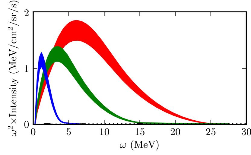
Figure 5: Incorrect spectral density obtained by using a purely ultrarelativistic approximation for the profile (29). Note that this is two orders of magnitude larger than the spectrum obtained from the full numerical solution (Fig. 4) and, if correct, would have easily ruled out our proposal. This serves to demonstrate the highly nontrivial nature of the predicted spectrum shown in Fig. 4 that is consistent with the observations [58].

Appendix B Debye Screening In the Electrosphere

Here we briefly discuss the plasma properties inside of the nugget’s electrosphere. The main point is that the Debye screening length $\lambda_{D}$ is much smaller than the typical de Broglie wavelength $\lambda=\hbar/p$ of electrons. Thus, the electric fields – although quite strong in the nugget’s electrosphere – will not appreciably effect the motion of electrons within the electrosphere as the charge is almost completely screened on a scale $\sim\lambda_{D}$.

This screening effect was completely neglected in [51], which led the authors to erroneously conclude that all electrons will be repelled before direct annihilation can proceed. The overall charge (see Table 1) will repel incident electrons at long distances as discussed in Sec. IV.3, but neutral hydrogen will easily penetrate the electrosphere, at which point the screening becomes effective, allowing the electrons to penetrate deeply and annihilate as discussed in Sec. V.

To estimate the screening of an electron, we solve the Poisson equation with a $\delta^{3}(\vec{\bm{r}}-\vec{\bm{r}}_{0})$ function describing the electron at position $\vec{\bm{r}}_{0}$ (see also 2),

$$\nabla^{2}\phi(\vec{\bm{r}})=-4\pi e\left[n(\vec{\bm{r}})-\delta^{3}(\vec{\bm{r}}-\vec{\bm{r}}_{0})\right]$$ (40)

where $\phi(\vec{\bm{r}})$ is the electrostatic potential and $n(\vec{\bm{r}})$ is the density of positrons. As before, we exchange $\phi$ for $\mu$, the effective chemical potential (3). Now let $n_{0}(\vec{\bm{r}})$ and $\mu_{0}(\vec{\bm{r}})$ be the solutions discussed in Sec. IV.2 without the potential $\delta^{3}(\vec{\bm{r}}-\vec{\bm{r}}_{0})$. We may then describe the screening cloud by $\mu(\vec{\bm{r}})=\mu_{0}(\vec{\bm{r}})+\delta_{\mu}(\vec{\bm{r}})$ and $n(\vec{\bm{r}})=n_{0}(\vec{\bm{r}})+\delta_{n}(\vec{\bm{r}})$ where

$$\nabla^{2}\delta_{\mu}(\vec{\bm{r}})=4\pi e^{2}\left[\delta_{n}(\vec{\bm{r}})-\delta^{3}(\vec{\bm{r}}-\vec{\bm{r}}_{0})\right]\\ \approx 4\pi\alpha\left[\frac{\partial{n[\mu]}}{\partial{\mu}}\delta_{\mu}(\vec{\bm{r}})-\delta^{3}(\vec{\bm{r}}-\vec{\bm{r}}_{0})\right]$$ (41)

where $n[\mu]$ is given by (4b). If the density is sufficiently large compared to the screening cloud deviations, we may take $\partial{n}/\partial{\mu}$ to be a constant, in which case we may solve (41) analytically with the boundary conditions:

$$\lim_{\vec{\bm{r}}\rightarrow\vec{\bm{r}}_{0}}\delta_{\mu}(\vec{\bm{r}}) =\frac{4\pi\alpha}{\lVert{\vec{\bm{r}}-\vec{\bm{r}}_{0}}\rVert}, \lim_{\vec{\bm{r}}\rightarrow\infty}\delta_{\mu}(\vec{\bm{r}}) =0.$$ (42)

This gives the standard Debye screening solution

$$\delta_{\mu}(\vec{\bm{r}})=\frac{-4\pi\alpha}{\lVert{\vec{\bm{r}}-\vec{\bm{r}}_{0}}\rVert}\exp\left(-\frac{\lVert{\vec{\bm{r}}-\vec{\bm{r}}_{0}}\rVert}{\lambda_{D}}\right)$$ (43)

where the Debye screening length is

$$\lambda_{D}^{-2}=4\pi\alpha\frac{\partial{n[\mu]}}{\partial{\mu}}.$$ (44)

On distances larger than $\lambda_{D}$, the charge of the electron is effectively screened. In particular, we can neglect the influence of the external electric field on motion of the electron if $\lambda_{D}$ is small compared to the de Broglie wavelength $\lambda=\hbar/p$ of the electrons:

$$1\ll\frac{\lambda}{\lambda_{D}}\sim\frac{1}{mv}\sqrt{4\pi\alpha\frac{\partial{n[\mu]}}{\partial{\mu}}}.$$ (45)

In the ultrarelativistic limit (26), one has $\partial{n}/\partial{\mu}\approx\mu^{2}/\pi^{2}+T^{2}/3$ whereas in the Boltzmann limit (31), one has $\partial{n}/\partial{\mu}\approx n_{0}/T$.

The relevant electron velocity scale in our problem is $v\sim 10^{-3}c$ ($T\sim 1$ eV). This is the typical scale for electrons ionized from neutral hydrogen. For these electrons, one immediately sees that the screening becomes significant in the Boltzmann regime once the density is larger than

$$n_{0}\gg\frac{m^{2}v^{2}T}{4\pi\alpha}\sim 0.1n_{\textrm{B}}$$ (46)

$n_{\textrm{B}}=(mT/2\pi)^{3/2}$ is the typical density in the Boltzmann regime. The typical electric fields in this regime are $E\sim\nabla\phi\sim eT/2z_{\alpha}$, which yield an ionization potential of $V_{\text{ionize}}\sim eEa_{0}\sim\alpha Ta_{0}/2z_{\alpha}\sim 1$ meV $\ll 13$ eV. Thus, the ionization of incoming hydrogen will not occur until the density is much larger, by which point the screening will be highly efficient. Contrary to the arguments presented in [51], electrons depositive via neutral hydrogen can easily penetrate deeply into the electrosphere producing the direct-annihilation emissions discussed in Sec. V.

Finally, we point out that, in the ultrarelativistic regime, we may express (45) in terms of the Fermi momentum:

$$\frac{\lambda}{\lambda_{D}}\sim\frac{p_{F}}{p}\sqrt{\frac{\alpha}{\pi}}.$$ (47)

Thus, for highly energetic particles, screening is irrelevant. The would apply to the $\sim 5$ MeV positrons ejected from the core of the nuggets that we argued are responsible for the diffuse 10 keV emission [4]. These see the full electric field which is responsible for their deceleration and ultimately for the emission of their energy in the 10 keV band. This point is somewhat irrelevant, however, as the positron electrosphere of the antimatter nuggets cannot screen a positive charge (screening is only efficient for particles of the opposite charge than the ion constituents).

References

- [1] A. R. Zhitnitsky, jcap 10, 010 (May 2003), arXiv:hep-ph/0202161
- [2] D. H. Oaknin and A. Zhitnitsky, Phys. Rev. D 71, 023519 (Jan. 2005), arXiv:hep-ph/0309086
- [3] A. Zhitnitsky, Phys. Rev. D 74, 043515 (Aug. 2006), arXiv:astro-ph/0603064
- [4] M. M. Forbes and A. R. Zhitnitsky, jcap 0801, 023 (2008), arXiv:astro-ph/0611506
- [5] M. M. Forbes and A. R. Zhitnitsky, Phys. Rev. D 78, 083505 (2008), arXiv:0802.3830 [astro-ph]
- [6] K. Lawson and A. R. Zhitnitsky, jcap 0801, 022 (January 2008), arXiv:0704.3064 [astro-ph]
- [7] E. Witten, Phys. Rev. D 30, 272 (1984)
- [8] R. D. Peccei and H. R. Quinn, Phys. Rev. D 16, 1791 (1977)
- [9] S. Weinberg, Phys. Rev. Lett. 40, 223 (1978)
- [10] F. Wilczek, Phys. Rev. Lett. 40, 279 (1978)
- [11] J. E. Kim, Phys. Rev. Lett. 43, 103 (1979)
- [12] M. A. Shifman, A. I. Vainshtein, and V. I. Zakharov, Nucl. Phys. B166, 493 (1980)
- [13] M. Dine, W. Fischler, and M. Srednicki, Phys. Lett. B104, 199 (1981)
- [14] A. R. Zhitnitsky, Sov. J. Nucl. Phys. 31, 260 (1980)
- [15] M. Srednicki (2002), arXiv:hep-th/0210172
- [16] K. van Bibber and L. J. Rosenberg, Phys. Today 59N8, 30 (2006)
- [17] S. J. Asztalos, L. J. Rosenberg, K. van Bibber, P. Sikivie, and K. Zioutas, Ann. Rev. Nucl. Part. Sci. 56, 293 (2006)
- [18] A. Dolgov and A. R. Zhitnitsky, work in progress (2009)
- [19] D. Kharzeev and A. Zhitnitsky, Nucl. Phys. A797, 67 (2007), arXiv:0706.1026 [hep-ph]
- [20] S. A. Voloshin, “Testing chiral magnetic effect with central U+U collisions,” (2010), arXiv:1006.1020
- [21] B. I. Abelev, et al. (STAR Collaboration), Phys. Rev. C 81, 054908 (May 2010), arXiv:0909.1717
- [22] C. Amsler et al. (Particle Data Group), Phys. Lett. B667, 1 (2008)
- [23] E. T. Herrin, D. C. Rosenbaum, and V. L. Teplitz, Phys. Rev. D 73, 043511 (2006), arXiv:astro-ph/0505584
- [24] E. S. Abers, A. K. Bhatia, D. A. Dicus, W. W. Repko, D. C. Rosenbaum, and V. L. Teplitz, Phys. Rev. D 79, 023513 (2009), arXiv:0712.4300 [astro-ph]
- [25] E. W. Kolb and M. S. Turner, The Early Universe (Westview Press, 5500 Central Avenue, Boulder, Colorado, 80301, 1994)
- [26] J. Knödlseder, V. Lonjou, P. Jean, M. Allain, P. Mandrou, J.-P. Roques, G. Skinner, G. Vedrenne, P. von Ballmoos, G. Weidenspointner, P. Caraveo, B. Cordier, V. Schönfelder, and B. Teegarden, Astron. Astrophys. 411, L457 (2003), arXiv:astro-ph/0309442
- [27] J. F. Beacom and H. Yüksel, Phys. Rev. Lett. 97, 071102 (2006), arXiv:astro-ph/0512411
- [28] H. Yüksel, Nucl. Phys. B Proc. Suppl. 173, 83 (2006), arXiv:astro-ph/0609139
- [29] D. H. Oaknin and A. R. Zhitnitsky, Phys. Rev. Lett. 94, 101301 (2005), arXiv:hep-ph/0406146
- [30] A. Zhitnitsky, Phys. Rev. D 76, 103518 (2007), arXiv:astro-ph/0607361
- [31] M. P. Muno et al., Astrophys. J. 613, 326 (2004), arXiv:astro-ph/0402087
- [32] D. P. Finkbeiner, Astrophys. J. 614, 186 (2004), arXiv:astro-ph/0311547
- [33] D. P. Finkbeiner, G. I. Langston, and A. H. Minter, Astrophys. J. 617, 350 (2004), arXiv:astro-ph/0408292
- [34] D. Hooper, G. Zaharijas, D. P. Finkbeiner, and G. Dobler, Phys. Rev. D 77, 043511 (February 2007), arXiv:0709.3114 [astro-ph]
- [35] G. Dobler and D. P. Finkbeiner, Astrophys. J. 680, 1222 (June 2008), arXiv:0712.1038 [astro-ph]
- [36] R. E. Lingenfelter, J. C. Higdon, and R. E. Rothschild, Phys. Rev. Lett. 103, 031301 (Jul 2009), arXiv:0904.1025
- [37] E. Farhi and R. L. Jaffe, Phys. Rev. D 30, 2379 (Dec 1984)
- [38] J. Madsen, “Strangelets, Nuclearites, Q-balls–A Brief Overview,” Invited talk at Workshop on Exotic Physics with Neutrino Telescopes, Uppsala, Sweden, Sept. 2006 (2006), arXiv:astro-ph/0612740v1
- [39] J. Madsen, Journal of Physics G: Nuclear and Particle Physics 31, S833 (2005), arXiv:astro-ph/0411601v1
- [40] M. B. Christiansen and N. K. Glendenning, Phys. Rev. C 56, 2858 (Nov. 1997)
- [41] P. Jaikumar, S. Reddy, and A. W. Steiner, Phys. Rev. Lett. 96, 041101 (Jan. 2006), arXiv:nucl-th/0507055
- [42] M. G. Alford, K. Rajagopal, S. Reddy, and A. W. Steiner, Phys. Rev. D 73, 114016 (Jun. 2006), arXiv:hep-ph/0604134
- [43] I. N. Mishustin, L. M. Satarov, T. J. Burvenich, H. Stoecker, and W. Greiner, Phys. Rev. C 71, 035201 (Mar. 2005), arXiv:nucl-th/0404026
- [44] A. B. Larionov, I. N. Mishustin, L. M. Satarov, and W. Greiner, Phys. Rev. C 78, 014604 (Jul. 2008), arXiv:0802.1845 [nucl-th]
- [45] C. Alcock, E. Farhi, and A. Olinto, Astrophys. J. 310, 261 (1986)
- [46] C. Kettner, F. Weber, M. K. Weigel, and N. K. Glendenning, Phys. Rev. D 51, 1440 (1995)
- [47] K. S. Cheng and T. Harko, Astrophys. J. 596, 451 (2003), arXiv:astro-ph/0306482
- [48] V. V. Usov, T. Harko, and K. S. Cheng, Astrophys. J. 620, 915 (2005), arXiv:astro-ph/0410682
- [49] H. Heiselberg, Phys. Rev. D 48, 1418 (Aug. 1993)
- [50] L. D. Landau and E. M. Lifshitz, Quantum Mechanics: Non-relativistic theory, 3rd ed., Course of Theoretical Physics, Vol. 3 (Butterworth-Heinemann, Oxford, 2003, c1977)
- [51] D. T. Cumberbatch, J. Silk, and G. D. Starkman, Phys. Rev. D 77, 063522 (March 2008), arXiv:astro-ph/0606429
- [52] V. V. Usov, Phys. Rev. D 70, 067301 (September 2004), arXiv:astro-ph/0408217
- [53] K. Ferrière, W. Gillard, and P. Jean, Astron. & Astrophys. 467, 611 (2007), arXiv:astro-ph/0702532
- [54] J. Madsen, Phys. Rev. Lett. 100, 151102 (Apr. 2008), arXiv:0804.2140
- [55] G. Weidenspointner, C. R. Shrader, J. Knödlseder, P. Jean, V. Lonjou, N. Guessoum, R. Diehl, W. Gillard, M. Harris, G. Skinner, P. von Ballmoos, G. Vedrenne, J.-P. Roques, S. Schanne, P. Sizun, B. Teegarden, V. Schoenfelder, and C. Winkler, Astron. Astrophys. 450, 1013 (2006), arXiv:astro-ph/0601673
- [56] G. Weidenspointner, G. K. Skinner, P. Jean, J. Knödlseder, P. von Ballmoos, G. Bignam, R. Diehl, A. W. Strong, B. Cordier, S. Schanne, and C. Winkler, Nature 451, 159 (Jan. 2008)
- [57] P. Jean et al., Astron. Astrophys. 407, L55 (2003), arXiv:astro-ph/0309484
- [58] A. W. Strong, I. V. Moskalenko, and O. Reimer, Astrophys. J. 613, 962 (2004), arXiv:astro-ph/0406254
- [59] G. Weidenspointner, G. Skinner, P. Jean, J. Knödlseder, P. von Ballmoos, R. Diehl, A. Strong, B. Cordier, S. Schanne, and C. Winkler, New Astronomy Reviews 52, 454 (2008), ISSN 1387-6473, astronomy with Radioactivities. VI - Proceedings of International Workshop Held at Ringberg Castle of Max Planck Gesellschaft in Kreuth, Germany, 7-10 January 2008
- [60] T. A. Porter, I. V. Moskalenko, A. W. Strong, E. Orlando, and L. Bouchet, Astrophys. J. 682, 400 (2008), arXiv:0804.1774
- [61] P. Jaikumar, C. Gale, D. Page, and M. Prakash, Phys. Rev. D 70, 023004 (July 2004), arXiv:astro-ph/0403427
- [62] J.-F. Caron and A. R. Zhitnitsky, Phys. Rev. D 80, 123006 (Dec. 2009), arXiv:0907.4715 [astro-ph.HE] [astro-ph.HE]
- [63] J. Charbonneau and A. R. Zhitnitsky, jcap 2010, 010 (Aug. 2010), arXiv:0903.4450 [astro-ph.HE]
- [64] F. R. Urban and A. R. Zhitnitsky, Phys. Lett. B 688, 9 (Apr. 2010), arXiv:0906.2162 [gr-qc]
- [65] F. R. Urban and A. R. Zhitnitsky, Nucl. Phys. B 835, 135 (Apr. 2010), arXiv:0909.2684 [astro-ph.CO]
- [66] P. Hohenberg and W. Kohn, Phys. Rev. 136, B864 (Nov 1964)
- [67] E. Braaten, ApJ 392, 70 (Jun. 1992)
- [68] E. H. Lieb and B. Simon, Phys. Rev. Lett. 31, 681 (Sep 1973)
- [69] N. Prantzos, C. Boehm, A. M. Bykov, R. Diehl, K. Ferriere, N. Guessoum, P. Jean, J. Knoedlseder, A. Marcowith, I. V. Moskalenko, A. Strong, and G. Weidenspointner(2010), arXiv:1009.4620