Hamiltonian reduction for the magnetic dynamics in antiferromagnetic crystals

Abstract

The nonlinear spin dynamics in antiferromagnetic crystals is studied for the magnetic structures similar to that of hematite. For the case when only two magnetization vectors are non-zero and the Hamiltonian has an axial symmetry, a reduction to a Hamiltonian system with one degree of freedom is performed, based on the corresponding conservation law. The analysis of the phase portraits of this system provides tractable analytical and geometric descriptions of the regimes of nonlinear spin dynamics in the crystal.

I Introduction

The phenomenological method of describing the properties of crystals with magnetic order is based on attributing classical magnetization vectors $\vec{S}_{i}\ (i=1,\ldots n)$ to the magnetic sublattices of a crystal ($n$ is the number of the sublattices), Borovik . These vectors are subject to exchange interaction between themselves, anisotropic interaction with the crystal lattice, and, optionally, Zeeman interaction with external magnetic fields, AM . The dynamics of these magnetizations can be described via the corresponding Hamiltonian system. Generally, the latter is nonlinear and its solving presents substantial difficulties. In the regimes when the spin vectors are close to their equilibrium positions, the linear approximation can be used, which allows to obtain the spin wave spectra in a relatively straightforward manner. However, the general nonlinear dynamics of sublattice magnetizations is also of considerable interest, e.g. for nonlinear regimes of magnetic resonance. Hence there is a need for methods of qualitative and quantitative investigating those dynamics in various situations.

To this end, the analytical tools devised for the study of mechanical Hamiltonian systems can be employed. In the present paper we apply an approach based on the reduction of a Hamiltonian system to another Hamiltonian system of lower dimensionality. The key idea is the considering of a subalgebra of the Poisson algebra of dynamic variables. If a subalgebra contains the Hamiltonian or, more generally, the Hamiltonian depends on the elements of the subalgebra and several first integrals, then the elements of the subalgebra are subject to a new Hamiltonian system with a lower number of phase variables. It was Poincare who first performed a reduction of a similar type in the three-body problem (see Whit ). A reduction based on considering a Poisson subalgebra was applied to the magnetization dynamics in superfluid ${}^{3}He$ B in Golo , lowering the phase space dimensionality from 6 to 3.

In the present work we consider the class of Hamiltonians having an axial symmetry. As a main example we use the case described in the classical work by Dzyaloshinsky, Dzyal , – the Hamiltonian comprising the leading terms in the magnetic energy of the four sublattices of the antiferromagnetic crystal $\alpha$-$Fe_{2}O_{3}$. It belongs to rhombohedral system, having a third-order symmetry axis, Dzyal . The magnetic energy comprises exchange terms and several spin-lattice interaction terms, some of them corresponding to the so-called Dzyaloshinsky-Moriya field leading to week ferromagnetism of $\alpha$-$Fe_{2}O_{3}$ (other possibilities include weak additional antiferromagnetism – the case of $Cr_{2}O_{3}$ in Dzyal , and the distortion of magnetic structure described in MarTikh ). In our case, if only second-order terms and the largest fourth-order term are taken into account (see Dzyal , section "Ferromagnetism of $\alpha$-$Fe_{2}O_{3}$"), then the Hamiltonian is invariant with respect to the rotation about the axis of the crystal. This results into the sum of the longitude angles of the spins being a cyclic variable, i.e. not entering the Hamiltonian (for a proper choice of dynamic variables). This allows to perform a reduction to a Poisson subalgebra as outlined above, decreasing the number of phase variables by 2 units. In the case of $\alpha$-$Fe_{2}O_{3}$, where only the ferromagnetic vector and one antiferromagnetic vector are non-zero, this reduction leads to a system with one degree of freedom, which can be effectively investigated by means of phase portraits. That provides a detailed picture of the nonlinear regimes of the spin dynamics in the given approximation. The same results hold for the carbonates of Fe, Mn and Co with a difference only in the values of the parameters of the Hamiltonian.

II The Hamiltonian formulation

We follow the well-known paper Dzyal by Dzyaloshinsky for constructing the Hamiltonian system describing the spin dynamics in $\alpha$-$Fe_{2}O_{3}$. The unit cell of the crystal is rhombohedral. The crystal has 4 magnetic sublattices, and the four corresponding Fe ions in the unit cell lie on the body diagonal of the rhombohedron – the third order symmetry axis of the crystal. The magnetizations of the sublattices are denoted $\vec{s}_{1},\vec{s}_{2},\vec{s}_{3},\vec{s}_{4}$. The Poisson brackets between their components have the usual form of the brackets for angular momentum:

$$\{s_{i\alpha},s_{i\beta}\}=\varepsilon_{\alpha\beta\gamma}s_{i\gamma},\quad\{s_{i\alpha},s_{j\beta}\}=0,\ i\neq j,$$ (1)

where the Greek letters denote the Cartesian coordinates of the vectors (here and below repeated indices imply summation over 1,2,3). The degeneracy of these brackets leads to the existence of four Casimir functions $s_{i}^{2},\ i=1,\ldots,4$.

Following Dzyaloshinsky, we describe the magnetic ordering in terms of the following four vectors:

$$\begin{array}[]{lcl}\vec{m}=\vec{s}_{1}+\vec{s}_{2}+\vec{s}_{3}+\vec{s}_{4},\\ \vec{l}_{1}=\vec{s}_{1}-\vec{s}_{2}-\vec{s}_{3}+\vec{s}_{4},\\ \vec{l}_{2}=\vec{s}_{1}-\vec{s}_{2}+\vec{s}_{3}-\vec{s}_{4},\\ \vec{l}_{3}=\vec{s}_{1}+\vec{s}_{2}-\vec{s}_{3}-\vec{s}_{4}.\\ \end{array}$$

The vector $\vec{m}$, the total magnetic moment, corresponds to ferromagnetism (if it is the only non-zero vector, the ordering is ferromagnetic), the vectors $\vec{l}_{i}$ – to antiferromagnetism, each of them describing a particular pattern of antiferromagnetic ordering, Dzyal . The Poisson brackets for these variables, following from (1), read:

$$\{m_{\alpha},m_{\beta}\}=\varepsilon_{\alpha\beta\gamma}m_{\gamma},\quad\{m_{\alpha},l_{i\beta}\}=\varepsilon_{\alpha\beta\gamma}l_{i\gamma},\quad\{l_{i\alpha},l_{i\beta}\}=\varepsilon_{\alpha\beta\gamma}m_{\gamma},\quad\{l_{i\alpha},l_{j\beta}\}=\varepsilon_{ijk}\,\varepsilon_{\alpha\beta\gamma}\,l_{k\gamma},\ i\neq j,$$

At the temperatures close to that of the antiferromagnetic transition the magnetic energy can be expanded in powers of $\,\vec{m},\,\vec{l}_{i}$, as their values are small. Let us use the rectangular coordinate system with the z-axis directed along the axis of the crystal, the x-axis – along one of the second-order symmetry axes.

The form of the possible terms in the magnetic energy can be deduced from the analysis of the magnetic symmetry. A thorough description of this approach is given in AM . As is shown in Dzyal , in the case of $\alpha$-$Fe_{2}O_{3}$ symmetry restrictions lead to the following general form of the second-order terms in the magnetic energy of the system:

$$E=A_{1}\vec{l}_{1}^{2}+A_{2}\vec{l}_{2}^{2}+A_{3}\vec{l}_{3}^{2}+B\vec{m}^{2}+\alpha_{1}l_{1z}^{2}+\alpha_{2}l_{2z}^{2}+\alpha_{3}l_{3z}^{2}+b\,m_{z}^{2}+\beta_{1}(l_{1x}m_{y}-l_{1y}m_{x})+\beta_{2}(l_{2x}l_{3y}-l_{2y}l_{3x}).$$

Here the first four terms correspond to the exchange interaction, the other terms – to the relativistic spin-lattice interaction and the magnetic dipolar interaction. Experimental results show that in $\alpha$-$Fe_{2}O_{3}$ the antiferromagnetic structure corresponds to the vector $\vec{l}_{1}$, Dzyal , which means that in equilibrium approximately $\vec{s}_{1}=-\vec{s}_{2}=-\vec{s}_{3}=\vec{s}_{4}$. There is also weak ferromagnetism described by the vector $\vec{m}$. So, by physical considerations, the system can be restricted to only these two vectors, which leads to the Poisson brackets:

$$\{m_{\alpha},m_{\beta}\}=\varepsilon_{\alpha\beta\gamma}m_{\gamma},\quad\{m_{\alpha},l_{\beta}\}=\varepsilon_{\alpha\beta\gamma}l_{\gamma},\quad\{l_{\alpha},l_{\beta}\}=\varepsilon_{\alpha\beta\gamma}m_{\gamma},\quad$$ (2)

and the Hamiltonian, Dzyal :

$$H=\frac{A}{2}\,\vec{l}^{2}+\frac{B}{2}\,\vec{m}^{2}+\frac{\alpha}{2}\,l_{z}^{2}+\frac{b}{2}\,m_{z}^{2}+\beta\,(l_{x}m_{y}-l_{y}m_{x})+\frac{C}{4}\,\vec{l}^{4},$$ (3)

where $\vec{l}=\vec{l}_{1}$, the index 1 is omitted in all positions, and normalizing factors are introduced. It should be noted that this Hamiltonian has a forth-order term depending on the main magnetic vector $\vec{l}=\vec{l}_{1}$. This model will be the object of our consideration.

III Symmetry and reduction

It is easy to notice that the Hamiltonian (3) is invariant with respect to the rotation about the z-axis, i.e. the anisotropy axis. This leads to $m_{z}$ being a first integral. Indeed, calculation shows that $\dot{m}_{z}=\{m_{z},H\}=0$. Moreover, the Poisson algebra (2) has two Casimir functions:

$$(\vec{m}+\vec{l})^{2},\ \ (\vec{m}-\vec{l})^{2}.$$

To take advantage of these facts, let us introduce the following variables:

$$\vec{g}=\frac{\vec{m}+\vec{l}}{2},\ \ \vec{h}=\frac{\vec{m}-\vec{l}}{2},$$

which are simply $\vec{g}=\vec{s}_{1}+\vec{s}_{4},\ \vec{h}=\vec{s}_{2}+\vec{s}_{3}$ in terms of the sublattice magnetizations. Their Poisson brackets have the usual form for angular momentum:

$$\{g_{\alpha},g_{\beta}\}=\varepsilon_{\alpha\beta\gamma}g_{\gamma},\quad\{h_{\alpha},h_{\beta}\}=\varepsilon_{\alpha\beta\gamma}h_{\gamma},\quad\{g_{\alpha},h_{\beta}\}=0.$$

The structure of the Poisson algebra given above admits of a reduction that substantially simplifies investigating the dynamics of the system. The key point is to cast the Poisson brackets for vector dynamical variables in a form that relies on the scalar ones. The idea is essentially due to K. Pohlmeyer, Pohl , who employed it for studying the algebra of currents in field theory. In paper Golo the method was used to study the spin dynamics in the B-phase of superfluid ${}^{3}He$ in the regime of turned off magnetic field.

In our case the reduction is obtained through the following system of variables:

$$\begin{array}[]{lcl}\vec{g}=(\sqrt{g^{2}-g_{z}^{2}}\,\cos{\varphi_{g}},\ \sqrt{g^{2}-g_{z}^{2}}\,\sin{\varphi_{g}},g_{z}),\\ \vec{h}=(\sqrt{h^{2}-h_{z}^{2}}\,\cos{\varphi_{h}},\ \sqrt{h^{2}-h_{z}^{2}}\,\sin{\varphi_{h}},h_{z}).\end{array}$$

The new variables have the following sense: $g$ – the modulus of $\vec{g}$, $g_{z}$ – its z-component, and $\varphi_{g}$ – its longitude angle (in xy-plane).

Thus, we take into account the symmetry of the system and turn to the scalar quantities, necessary for the Pohlmeyer reduction. It is worthwhile to note that a similar transformation was used in papers Sriv1 , Reichl for studying chaotic dynamics in two-spin systems.

Using the reverse transformation:

$$g=\sqrt{g_{x}^{2}+g_{y}^{2}+g_{z}^{2}},\quad\varphi_{g}=\arctan{\frac{g_{y}}{g_{x}}},$$

we obtain the following Poisson brackets:

$$\begin{array}[]{lcl}\{\varphi_{g},g_{z}\}=1,\ \ \{g,g_{z}\}=0,\ \ \{g,\varphi_{g}\}=0,\\ \{\varphi_{h},h_{z}\}=1,\ \ \{h,h_{z}\}=0,\ \ \{h,\varphi_{h}\}=0,\end{array}$$

all the g–h brackets being zero.

Thus, we have got two advantages. The first one is the lowering of the phase space dimensionality by two units, as $g$ and $h$ are Casimir functions, and their values can be fixed. Therefore, we have a system with two pairs of canonically conjugate variables: $\varphi_{g},g_{z}$ and $\varphi_{h},h_{z}$. The second one is that we can easily employ the fact that $m_{z}=g_{z}+h_{z}$ is a first integral. Indeed, another formulation of this is that the system is invariant with respect to the rotation about the z-axis. This means that the Hamiltonian should depend only on the difference of the angles $\varphi_{g}-\varphi_{h}$, not on their specific values. In fact, calculation of the Hamiltonian after the above transformations gives:

$$\begin{array}[]{lcl}\displaystyle H=\frac{1}{2}\,A\left[-2\sqrt{g^{2}-g_{z}^{2}}\sqrt{h^{2}-h_{z}^{2}}\,\cos{(\varphi_{g}-\varphi_{h})}-2g_{z}h_{z}+g^{2}+h^{2}\right]+\\ +\frac{1}{2}\,B\left[2\sqrt{g^{2}-g_{z}^{2}}\sqrt{h^{2}-h_{z}^{2}}\,\cos{(\varphi_{g}-\varphi_{h})}+2g_{z}h_{z}+g^{2}+h^{2}\right]+\\ +\frac{1}{2}\,\alpha\,(g_{z}-h_{z})^{2}+\frac{1}{2}\,b\,(g_{z}+h_{z})^{2}-2\beta\,\sqrt{g^{2}-g_{z}^{2}}\sqrt{h^{2}-h_{z}^{2}}\,\sin{(\varphi_{g}-\varphi_{h})}+\\ +\frac{1}{4}\,C\left[-2\sqrt{g^{2}-g_{z}^{2}}\sqrt{h^{2}-h_{z}^{2}}\cos{(\varphi_{g}-\varphi_{h})}-2g_{z}h_{z}+g^{2}+h^{2}\right]^{2}.\end{array}$$

Applying the canonical transformation:

$$\begin{array}[]{lcl}u=\displaystyle\frac{\varphi_{g}-\varphi_{h}}{\sqrt{2}},\ \ p_{u}=\frac{g_{z}-h_{z}}{\sqrt{2}},\\ v=\displaystyle\frac{\varphi_{g}+\varphi_{h}}{\sqrt{2}},\ \ p_{v}=\frac{g_{z}+h_{z}}{\sqrt{2}},\\ \end{array}$$

we obtain the Hamiltonian:

$$\begin{array}[]{lcl}H=\par\frac{1}{2}A\left(-\cos\left(\sqrt{2}u\right)\sqrt{2g^{2}-\left(p_{u}+p_{v}\right){}^{2}}\sqrt{2h^{2}-\left(p_{u}-p_{v}\right){}^{2}}+g^{2}+h^{2}+p_{u}^{2}-p_{v}^{2}\right)\\ +\frac{1}{2}B\left(\cos\left(\sqrt{2}u\right)\sqrt{2g^{2}-\left(p_{u}+p_{v}\right){}^{2}}\sqrt{2h^{2}-\left(p_{u}-p_{v}\right){}^{2}}+g^{2}+h^{2}-p_{u}^{2}+p_{v}^{2}\right)\\ +\alpha p_{u}^{2}+bp_{v}^{2}-\beta\sin\left(\sqrt{2}u\right)\sqrt{2g^{2}-\left(p_{u}+p_{v}\right){}^{2}}\sqrt{2h^{2}-\left(p_{u}-p_{v}\right){}^{2}}\\ +\frac{1}{4}C\left(-\cos\left(\sqrt{2}u\right)\sqrt{2g^{2}-\left(p_{u}+p_{v}\right){}^{2}}\sqrt{2h^{2}-\left(p_{u}-p_{v}\right){}^{2}}+g^{2}+h^{2}+p_{u}^{2}-p_{v}^{2}\right){}^{2}.\\ \end{array}$$ (4)

It is easy to see that $v$ does not enter this function. So, as noted above, $p_{v}$ is a first integral, and as the variables $u,p_{u}$ have zero Poisson brackets with it, we conclude that the Hamiltonian 4 defines a separate Hamiltonian system in variables $u,p_{u}$ only. In other words, after fixing the integrals of motion the function 4 becomes a member of the Poisson subalgebra of dynamic variables generated by $u,p_{u}$ and the first integrals, thus defining Hamiltonian dynamics within this subalgebra.

The study of the dynamics of our system then proceeds as follows. Firstly, we study phase pictures of the reduced system for $u,p_{u}$. Secondly, we consider the "lift" of the obtained two-dimensional dynamics to the six-dimensional space of the initial spin variables. Results obtained in this way admit of graphic representation.

The dynamical regimes of the reduced system can be studied by means of phase portraits in the $u\,-\,p_{u}$ phase plane. A typical portrait is shown in fig. 1. It contains several fixed points: centers and saddles, and separatrices, each of which either connects a pairs of saddles or forms a loop having the origin and the end in the same saddle.

A typical trajectory going around a center not far from it is shown in figs. 2, 3 in the spaces of the vectors $\vec{l}$, $\vec{m}$ respectively; a trajectory close to a separatrix – in figs. 4, 5. It’s easy to see that stationary points in the phase portrait correspond to horizontal circles in the spaces of the magnetic vectors $\vec{l}$, $\vec{m}$, i.e. to circular precession of these vectors. Other trajectories manifest more complicated behaviour, as can be seen in figs. 6, 7.

An especially interesting example is a trajectory going very close to a separatrix. This means that for a long period of time it approaches a saddle point, manifesting roughly circular precession of magnetizations, but at a certain moment it starts moving away from that saddle performing some complicated dynamics before reaching another almost-steady regime of circular precession.

The author is grateful to prof. V.L. Golo for constant attention to this work.

The author acknowledges prof. V.I. Marchenko for useful communications.

The work was supported by the grants RFFI 09-02-00551, 09-03-00779.

Figure 1: A typical phase portrait of the system for the variables $u,\ p_{u}=l_{z}/\sqrt{2}$.

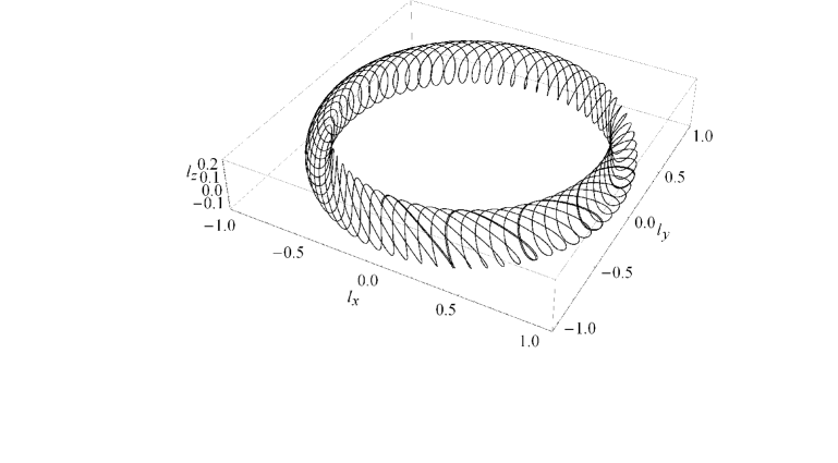
Figure 2: A trajectory surrounding a center (elliptic fixed point) in the phase portrait (fig. 1), shown in the space of the coordinates of the antiferromagnetic vector $\vec{l}$. The curve is winding over a 2D-torus.

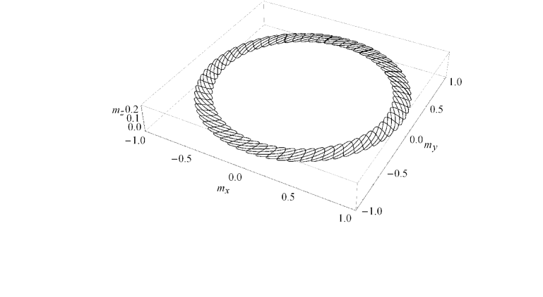
Figure 3: A trajectory surrounding a center (elliptic fixed point) in the phase portrait (fig. 1), shown in the space of the coordinates of the ferromagnetic vector $\vec{m}$. The curve is confined to a horizontal plane $m_{z}=const$.

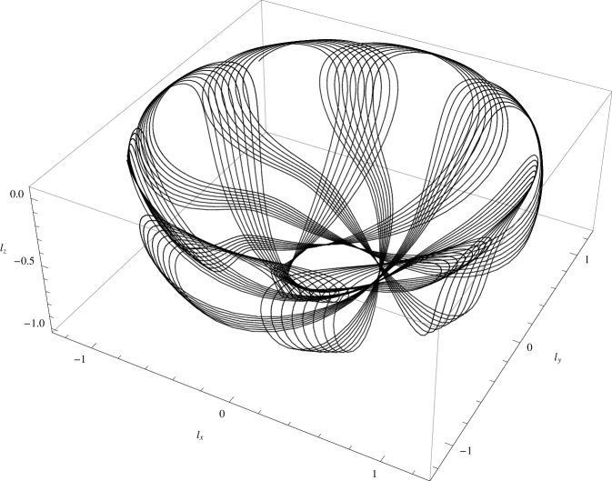
Figure 4: A trajectory close to a separatrix connecting two saddles in the phase portrait (fig. 1), shown in the space of the coordinates of the antiferromagnetic vector $\vec{l}$. The vector migrates between two horizontal circles corresponding to the two saddles.

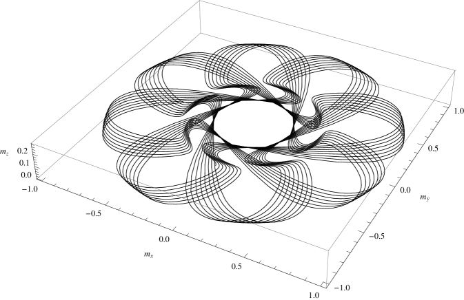
Figure 5: A trajectory close to a separatrix connecting two saddles in the phase portrait (fig. 1), shown in the space of the coordinates of the ferromagnetic vector $\vec{m}$. The vector migrates between two circles corresponding to the two saddles. The curve is confined to a horizontal plane $m_{z}=const$.

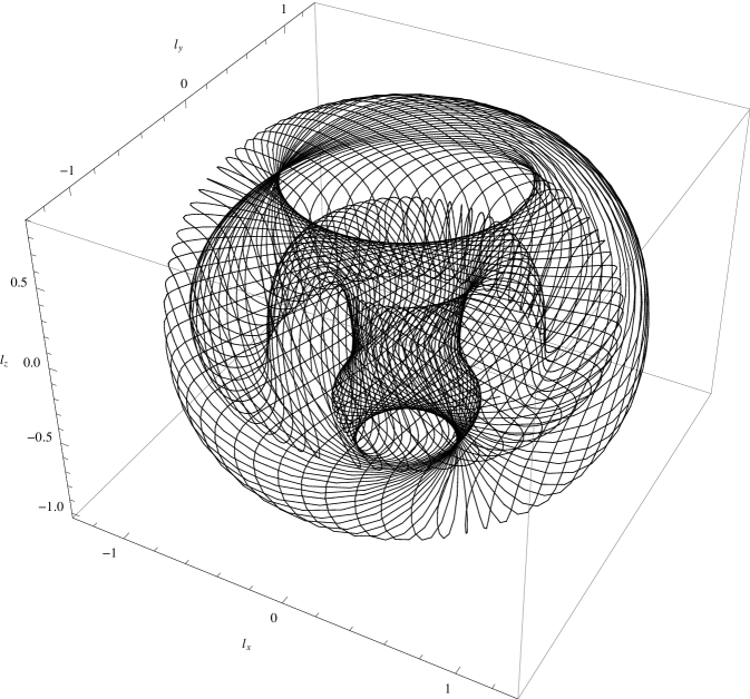
Figure 6: A trajectory taking S-shaped path between several centers and saddles in the phase portrait (fig. 1), shown in the space of the coordinates of the antiferromagnetic vector $\vec{l}$.

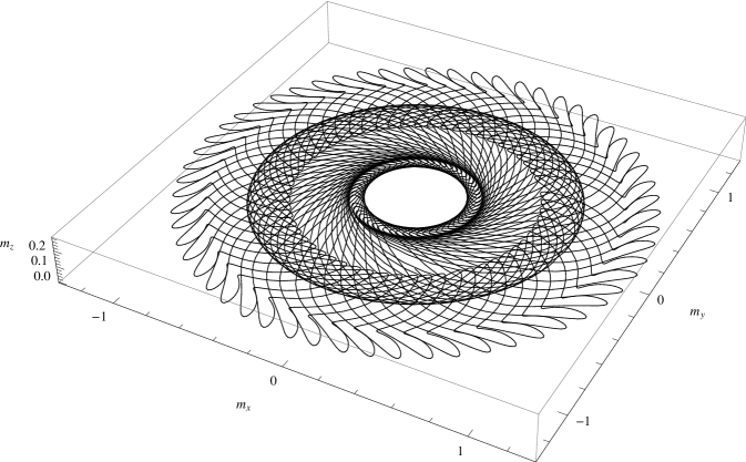
Figure 7: A trajectory taking S-shaped path between several centers and saddles in the phase portrait (fig. 1), shown in the space of the coordinates of the ferromagnetic vector $\vec{m}$. The curve is confined to a horizontal plane $m_{z}=const$.

References

- (1) A.F. Andreev and V.I. Marchenko, Symmetry and the macroscopic dynamics of magnetic materials, Sov. Phys. Usp., 23 (1), pp. 21-34 (1980).
- (2) E.S. Borovik, V.V. Eremenko, A.S. Milner, Lectures on Magnetism, Physmathlit, Moscow (2005).
- (3) I. Dzyaloshinsky, A thermodynamic theory of ‘‘weak’’ ferromagnetism of antiferromagnetics, Journal of Physics and Chemistry of Solids, vol. 4, issue 4, pp. 241-255 (1957).
- (4) E.T. Whittaker, A Treatise on the Analytical Dynamics of Particles and Rigid Bodies, Cambridge University Press, 4th edition (1989).
- (5) K. Pohlmeyer, Integrable hamiltonian systems and interactions through quadratic constraints, Comm. math, phys., 46, 207-221 (1976).
- (6) V.L. Golo, Nonlinear regimes in spin dynamics of superfluid 3He, Letters in Mathematical Physics, Vol. 5, N. 2 (1981).
- (7) V.I. Marchenko, A.M. Tikhonov, On the NMR spectrum in antiferromagnetic , JETP Lett., 69, p. 44 (1999).
- (8) N. Srivastava, C. Kaufman, G. Müller, R. Weber and H. Thomas, Integrable and nonintegrable classical spin clusters, Z. Phys. B 70, pp. 251-268 (1988).
- (9) D.T. Robb and L.E. Reichl, Chaos in a two-spin system with applied magnetic field, Phys. Rev. E 57, N. 2, pp. 2458-2459 (1998).