Entanglement optimizing mixtures of two-qubit states

Abstract

Entanglement in incoherent mixtures of pure states of two qubits is considered via the concurrence measure. A set of pure states is optimal if the concurrence for any mixture of them is the weighted sum of the concurrences of the generating states. When two or three pure real states are mixed it is shown that $28.5\%$ and $5.12\%$ of the cases respectively, are optimal. Conditions that are obeyed by the pure states generating such optimally entangled mixtures are derived. For four or more pure states it is shown that there are no such sets of real states. The implications of these on superposition of two or more dimerized states is discussed. A corollary of these results also show in how many cases rebit concurrence can be the same as that of qubit concurrence.

I Introduction

Entanglement properties of pure and mixed quantum states have been the subject of intense and extensive study in the recent past Horodecki09 . Of these, entanglement in qubits or spin-1/2 systems have dominated due to their use as fundamental objects in quantum computations. For an arbitrary state of two qubits the concurrence measure (or its square, called tangle) introduced by Hill and Wootters Wootters is simply calculable from the density matrix and is a measure of entanglement. To be precise the entanglement of formation Nielsen is a monotonic function of the concurrence. The concurrence measure has been extensively applied in many physical contexts, for instance in the study of quantum phase transitions Nature . In a collection of qubits, concurrence measures the entanglement present within any chosen pair. Thus due to the monogamy property of entanglement monogamy it is reasonable to expect that states with large multipartite entanglement have low or vanishing concurrence. In fact for a random state with more than six qubits the probability that a chosen pair has nonzero concurrence is vanishingly small, most of the entanglement is of the multipartite kind Kendon02 ; ScottCaves .

To elaborate on this property, consider a mixed state of two qubits

$$\rho=\sum_{i=1}^{k}p_{i}\,|\psi_{i}\rangle\langle\psi_{i}|,\;\;k>1,$$ (1)

where $p_{i}\geq 0$, $\sum_{i}p_{i}=1$ and the projectors are arbitrary, in particular, $|\psi_{i}\rangle\langle\psi_{i}|$ need not be orthogonal. The convexity of concurrence Uhlmann00 implies that

$$C(\rho)\leq\sum_{i=1}^{k}p_{i}C(\psi_{i})$$ (2)

where $C$ is the concurrence function, an entanglement monotone Wootters . Thus the maximum that $C(\rho)$ can attain is the weighted sum of the concurrence of the extremal (pure) states. If there exists a set $\{|\psi_{1}\rangle,\cdots,\psi_{k}\rangle\}$ such that equality is obtained in Eq. (2) for any arbitrary set of weights $\{p_{i}\}$, it is referred to herein as optimal. However note that such a property will be specific to the concurrence measure of entanglement.

For states that are real in the standard basis, it is shown that a very large fraction of states made by incoherently superposing 2 two-qubit states optimize their entanglement. This property is analyzed in detail in this paper and conditions to be satisfied by the extremal states such that the resultant density matrix is optimal are derived. Any real density matrix can be tested for optimality of its diagonal decomposition using the inequalities derived. These are also generalized beyond two states, and it is shown that for more than three real states, not one optimal decomposition exists.

The relevance to superposed dimers will be studied in section III. The relation between entanglement and superpostion of quantum states is an interesting one Linden . Indeed superposition of states with a tensor product structure is necessary for entanglement, however of course this is not sufficient. There is a significant amount of literature establishing bounds on various entanglement measures for the superposition in terms of the entanglement in the states that are being so superposed Nisert ; Linden ; Chang ; Heng ; Gour ; Song ; Osterloh .

II Rank-wise study of optimizing mixtures

If two pure and real states $|\psi_{1}\rangle$ and $|\psi_{2}\rangle$ are chosen at random, it is shown in this paper that in $28.5\%$ of cases the resultant entanglement in $p|\psi_{1}\rangle\langle\psi_{1}|+(1-p)|\psi_{2}\rangle\langle\psi_{2}|$ is the maximum possible, namely equality holds in Eq. (2). This implies that on superposing 2 two-qubit states, $28.5\%$ of the states will remain entangled optimally, as defined in the introduction. The fraction $0.285$ of optimal pairs is interesting and strong evidence that it is actually $(\pi-2)/4$ is presented in an Appendix.

The conditions under which such optimality occurs is now obtained, however this is done in a more general setting in what follows. In particular, extending these results to arbitrary mixtures of three real pure states, one finds that in about $5.1\%$ of cases this gives rise to optimally entangled states. It is also then shown that for four or more states there is not even one set of pure real states, such that all their mixtures are optimal. These generalizations are of relevance when more than 2 two-qubit states are superposed.

The reader is first reminded of the procedure to find the concurrence in $\rho$, a given state of two qubits Wootters . The spin-flipped state $\tilde{\rho}=\sigma_{y}\otimes\sigma_{y}\rho^{*}\sigma_{y}\otimes\sigma_{y}$ is found, where the complex conjugation is done in the standard basis. Then the matrix $\rho\tilde{\rho}$ is diagonalized and has positive eigenvalues $\mu_{1}\geq\mu_{2}\geq\mu_{3}\geq\mu_{4}$. The concurrence $C(\rho)$ is $\mbox{max}(0,\sqrt{\mu_{1}}-\sqrt{\mu_{2}}-\sqrt{\mu_{3}}-\sqrt{\mu_{4}})$.

This somewhat involved definition of the concurrence renders it opaque for considerations of optimality. However it is possible to express the concurrence of $\rho=\sum_{i=1}^{k}p_{i}|\psi_{i}\rangle\langle\psi_{i}|$ more explicitly in terms of the the states $|\psi_{i}\rangle$ and the weights $p_{i}$. Restrict to the case $k\leq 4$, that is the size of the generating set of states is not larger than the maximum rank of $\rho$. Note that if any $\rho$ is expressed in its eigenbasis this is not a restriction at all. It is now shown that the eigenvalues of $\rho\tilde{\rho}$ are the same as that of $r^{\prime}r^{\prime*}$ where

$$r^{\prime}_{ij}=\sqrt{p_{i}p_{j}}\,r_{ij},\;\mbox{and}\;r_{ij}=\langle\psi_{i}|\sigma_{y}\otimes\sigma_{y}|\psi_{j}^{*}\rangle.$$ (3)

Thus rather than using the density matrix directly, the pure states comprising a particular ensemble are used. Note that $|r_{11}|$ and $|r_{22}|$ are the concurrences, $C(\psi_{1})$ and $C(\psi_{2})$, of the pure states $|\psi_{1}\rangle$ and $|\psi_{2}\rangle$ respectively.

For convenience the eigenvalue equation for $\tilde{\rho}\rho$ is considered, whose right eigenvectors can be written in the nonorthogonal, sub-normalized basis of the extremal states as $|\nu\rangle=\sum_{i}\alpha_{i}|\psi_{i}^{\prime}\rangle$, where $|\psi_{i}^{\prime}\rangle=\sqrt{p_{i}}|\psi_{i}\rangle$. Also, writing $\rho=\sum_{i=1}^{k}|\psi_{i}^{{}^{\prime}}\rangle\langle\psi_{i}^{{}^{\prime}}|$ and using the fact that $\langle\psi_{m}^{{}^{\prime}}|\tilde{\rho}\rho|\nu\rangle=\mu\langle\psi_{m}^{{}^{\prime}}|\nu\rangle$ results in

$$\sum_{i=1}^{k}(\sum_{j=1}^{k}\tilde{\rho^{\prime}}_{mj}t_{ji}^{\prime}-\mu t_{mi}^{\prime})\alpha_{i}=0,\;\;1\leq m\leq k,$$ (4)

where

$$t^{\prime}_{ji}=\sqrt{p_{j}p_{i}}\;t_{ji}=\sqrt{p_{j}p_{i}}\langle\psi_{j}|\psi_{i}\rangle$$ (5)

is a matrix of inner products (the Gram matrix) and

$$\tilde{\rho^{\prime}}_{mj}=\sqrt{p_{m}p_{j}}\;\tilde{\rho}_{mj}=\sqrt{p_{m}p_{j}}\langle\psi_{m}|\tilde{\rho}|\psi_{j}\rangle.$$ (6)

Note also that since, $\rho^{*}=\sum p_{i}|\psi_{i}^{*}\rangle\langle\psi_{i}^{*}|$,

$$\tilde{\rho^{{}^{\prime}}}_{mj}=\langle\psi_{m}^{{}^{\prime}}|\tilde{\rho}|\psi_{j}^{{}^{\prime}}\rangle=\langle\psi_{m}^{{}^{\prime}}|\sigma_{y}\otimes\sigma_{y}(\sum p_{i}|\psi_{i}^{*}\rangle\langle\psi_{i}^{*}|)\sigma_{y}\otimes\sigma_{y}|\psi_{j}^{{}^{\prime}}\rangle$$ (7)

the following matrix identity is readily derived: $\tilde{\rho^{\prime}}=r^{\prime}r^{\prime*}=r^{\prime}r^{\prime\dagger}$, where $r$ and $r^{\prime}$ are defined above in Eq. (3).

For the $k$ equations in Eq.(4) to have non-trivial solutions $\det(\Lambda)=0$, where

$$\Lambda_{mi}=(\tilde{\rho^{{}^{\prime}}}t^{\prime})_{mi}-\mu(t^{\prime})_{mi},$$ (8)

which further implies that

$$\det(t^{\prime})\,\det(r^{\prime}r^{\prime*}-\mu I)=0.$$ (9)

As the number of vectors $|\psi_{i}\rangle$ are no larger in number than the dimensionality of the Hilbert space, we assume them to be independent and therefore $\det(t^{\prime})=p_{1}\cdots p_{k}\det(t)\neq 0$. Thus

$$\det(r^{\prime}r^{\prime*}-\mu I)=0.$$ (10)

and hence the characteristic polynomials of $\rho\tilde{\rho}$ and $r^{\prime}r^{\prime*}$ are identical.

If the state $\rho$ is real in the computational basis then the eigenvalue problem of $r^{\prime}r^{\prime*}$ is that of $r^{\prime 2}$, whose eigenvalues are the square of the eigenvalues of $r^{\prime}$, which are indicated as $\lambda$. The expression for concurrence is derived and the conditions for optimality are now considered case-by-case starting from $k=2$.

II.1 Rank-2 density matrices: ${\mathbf{k}=2}$

For the case of mixtures of two real pure states, $k=2$, the above considerations lead to the following characteristic equation of $r^{\prime}$ (as defined in Eq. (3)):

$$\lambda^{2}-\xi\lambda+p_{1}p_{2}\chi_{12}=0$$ (11)

where $\xi=p_{1}r_{11}+p_{2}r_{22}$, and $\chi_{12}=(r_{11}r_{22}-r_{12}^{2})$. The eigenvalues are therefore

$$\lambda_{\pm}=\frac{1}{2}(\xi\pm\sqrt{\xi^{2}-4p_{1}p_{2}\chi_{12}})$$ (12)

If $\chi_{12}>0$ and $\xi>0$ then $\lambda_{+}>\lambda_{-}>0$, and $C(\rho)=\lambda_{+}-\lambda_{-}$. Alternatively if $\chi_{12}>0$ and $\xi<0$ then $\lambda_{-}<\lambda_{+}<0$, and $C(\rho)=|\lambda_{-}|-|\lambda_{+}|$. Thus if $\chi_{12}>0$, irrespective of the sign of $\xi$, we have that

$$C(\rho)=\sqrt{\xi^{2}-4p_{1}p_{2}\chi_{12}}<|\xi|<p_{1}C(\psi_{1})+p_{2}C(\psi_{2}),$$ (13)

confirming the convexity of concurrence.

The case $\chi_{12}<0$ is more interesting and leads to optimality. If $\xi>0$ then $\lambda_{-}<0<\lambda_{+}$ and $\lambda_{+}>|\lambda_{-}|$. It follows that $C(\rho)=\lambda_{+}-|\lambda_{-}|=\lambda_{+}+\lambda_{-}=\xi$. Combining a similar analysis of the case $\xi<0$ one gets that when $\chi_{12}<0$, irrespective of the sign of $\xi$

$$C(\rho)=|\xi|=|p_{1}r_{11}+p_{2}r_{22}|.$$ (14)

This brings us to the possibility that if $r_{11}r_{22}>0$ then $C(\rho)=p_{1}C(\psi_{1})+p_{2}C(\psi_{2}).$ Thus when $|\psi_{1}\rangle$ and $|\psi_{2}\rangle$ satisfy the conditions that $r_{11}r_{22}>0$ and $r_{11}r_{22}-r_{12}^{2}<0$ any arbitrary mixture of these pure states has the maximum entanglement which is their average entanglement. This is the first set of optimality conditions that we derive.

The set of such optimal states is a subset from pairs of real states. Each real state of two qubits is characterized by $4$ real coefficients, say $x_{i}$, $i=1,\ldots,4$. The normalization condition means that there is a isomorphism between these and the 3-sphere $x_{1}^{2}+x_{2}^{2}+x_{3}^{2}+x_{4}^{2}=1$. Apart from the fact that states differing by a sign are really the same (thus the space is a projective space) the states maybe thought of as points in $S^{3}$. Thus a pair of real states is a point on the manifold $S^{3}\times S^{3}$, and the set of optimal states forms a subset therein whose fractional volume is of natural interest.

Assume that the real states of two qubits are distributed uniformly on $S^{3}$, namely choose the Haar measure. Equivalently, the probability density of random real pure states Brody of two qubits is given by

$$P(\{x_{i}\})=\dfrac{1}{\pi^{2}}\delta\left(\sum_{i=1}^{4}x_{i}^{2}-1\right),$$ (15)

where $x_{i}$ are the state components in a generic basis such as the computational one. The fraction of optimal states $f_{2}$ is then the following integral on $S^{3}\times S^{3}$, written in terms of the ambient space components $(x_{i},y_{i}$) of $\mathbb{R}^{4}\times\mathbb{R}^{4}$:

$$f_{2}=\int\Theta(r_{11}r_{22})\Theta(r_{12}^{2}-r_{11}r_{22})P(\{x_{i}\})P(\{y_{i}\})\prod_{i=1}^{4}dx_{i}dy_{i}.$$ (16)

Here $r_{11}=\langle\psi_{1}|\sigma_{y}\otimes\sigma_{y}|\psi_{1}\rangle=2(x_{2}x_{3}-x_{1}x_{4})$, $r_{22}=\langle\psi_{2}|\sigma_{y}\otimes\sigma_{y}|\psi_{2}\rangle=2(y_{2}y_{3}-y_{1}y_{4})$, $r_{12}=\langle\psi_{1}|\sigma_{y}\otimes\sigma_{y}|\psi_{2}\rangle=x_{2}y_{3}+y_{2}x_{3}-x_{1}y_{4}-x_{4}y_{1}$, and $\Theta$ is the Heaviside step function that is $1$ if its argument is positive and zero otherwise. An exact evaluation of this integral seems possible and equal to $(\pi-2)/4$ (see the Appendix), however it is quite easy to simulate the process by choosing two independent vectors ${x_{i}}$ and ${y_{i}}$ distributed according to Eq. (15) and checking to see if the optimality condition is satisfied. The initial choice of vectors is done by simply taking $4$ numbers from any zero centered normally distributed set and normalizing them. This procedure gives the fraction $f_{2}$ to be approximately $0.285$, in good agreement with the value of $(\pi-2)/4$.

II.2 Rank-3 density matrices: ${\mathbf{k}=3}$

Now we consider the general setting of mixing three real pure states, $k=3$, which leads to the cubic equation for the eigenvalues of $r^{\prime}$, (defined in Eq. (3)):

$$f(\lambda)=\lambda^{3}+\xi_{1}\lambda^{2}+\xi_{2}\lambda+\xi_{3}=0,$$ (17)

where the coefficients $\xi_{i}$ are

$$\xi_{1}=-\sum_{i}p_{i}r_{ii},\;\xi_{2}=\sum_{i\neq j}p_{i}p_{j}(r_{ii}r_{jj}-r_{ij}^{2}),\;\xi_{3}=-p_{1}p_{2}p_{3}\,\det(r).$$ (18)

Now we state two Lemmas which are key to understanding the nature of the roots of cubic equations and the possibility of optimal states in the case $k=3$.

Lemma 1.

If $p(x)$ is a cubic in $x$, $p(x)=x^{3}+ax^{2}+bx+c$ with real coefficients, has real roots, and is such that $a,b,c<0$ then $p(x)=0$ has two negative roots and one positive root with the positive root being greater than the other two in modulus.

Proof.

Since $c<0$ the product of the roots is positive which implies that either all roots are positive or there are two negative and one positive root. However since $b<0$ the quadratic $p^{\prime}(x)$ has one positive and one negative root. Hence all the roots of $p(x)$ cannot be positive since the roots of $p^{\prime}(x)$ have to lie between the roots of $p(x)$ by Cauchy’s mean value theorem for differentiable functions. Hence the polynomial has two negative and one positive root. Observe that $a<0$ implies the sum of the roots is positive which implies that the positive root has the largest modulus. ∎

Lemma 2.

If $p(x)$ be a cubic in $x$, $p(x)=x^{3}+ax^{2}+bx+c$ with real coefficients and has real roots, and is such that $b<0$ and $a,c>0$ then the cubic has two positive roots and one negative root with the negative root being greater than the other two in modulus.

Proof.

The proof of this lemma is on similar lines to the previous one. ∎

Case 1. Now suppose we have $\xi_{1},\xi_{3}<0$ then along with the condition that $\xi_{2}<0$ we have by Lemma 1 that the characteristic equation has two negative and one positive root and that the positive root has the largest magnitude. Without loss of generality let us assume that $\lambda_{1}>0$ then we have the square-roots of the eigenvalues of $\rho\tilde{\rho}=(\sigma_{y}\otimes\sigma_{y}\,\rho)^{2}$ are $\lambda_{1},-\lambda_{2},-\lambda_{3}$. Hence the concurrence of $\rho$ is $C(\rho)=\mbox{max}(0,\lambda_{1}+\lambda_{2}+\lambda_{3})=\mbox{max}(0,-\xi_{1})=|\xi_{1}|$. Thus

$$C(\rho)=p_{1}r_{11}+p_{2}r_{22}+p_{3}r_{33}.$$ (19)

If we have $r_{ii}>0$ for $i=1,2,3$ then clearly $C(\psi_{i})=r_{ii}$. Also if $\xi_{2}<0$ then since $p_{i}$’s can be arbitrary positive reals bounded by 1 we have each term $p_{i}p_{j}(r_{ii}r_{jj}-r^{2}_{ij})<0$ which means $r_{ii}r_{jj}-r^{2}_{ij}<0,i\neq j$ is a necessary condition. Thus we have that if

$$r_{ii}>0,r_{ii}r_{jj}-r^{2}_{ij}<0,i\neq j$$ (20)

and

$$\det(r)=\sum_{cyc}r_{11}(r_{22}r_{33}-r_{13}^{2})-2(r_{11}r_{22}r_{33}-r_{12}r_{23}r_{31})>0$$ (21)

then any mixture of the triple $\{|\psi_{1}\rangle,|\psi_{2}\rangle,|\psi_{3}\rangle\}$ will be optimally entangled, that is

$$C(\rho)=\sum_{i=1}^{3}p_{i}C(\psi_{i})$$ (22)

Case 2. Similarly suppose we have $\xi_{1},\xi_{3}>0$ then along with the condition that $\xi_{2}<0$ we have by Lemma 2 that the characteristic equation has two positive and one negative root and that the negative root has the largest magnitude. Let us assume that $\lambda_{1}<0$ then we have that the square-roots of the eigenvalues of $\rho\tilde{\rho}=(\sigma_{y}\otimes\sigma_{y}\,\rho)^{2}$ are $-\lambda_{1},\lambda_{2},\lambda_{3}$. Hence the concurrence of $\rho$ $C(\rho)=\mbox{max}(0,-(\lambda_{1}+\lambda_{2}+\lambda_{3}))=\mbox{max}(0,\xi_{1})=\xi_{1}$, since $\xi_{1}>0$. Thus we have if

$$r_{ii}<0,r_{ii}r_{jj}-r^{2}_{ij}<0,i\neq j$$ (23)

and

$$\det(r)=\sum_{cyc}r_{11}(r_{22}r_{33}-r_{13}^{2})-2(r_{11}r_{22}r_{33}-r_{12}r_{23}r_{31})<0$$ (24)

then again any mixture of the triple $\{|\psi_{1}\rangle,|\psi_{2}\rangle,|\psi_{3}\rangle\}$ is optimally entangled. These conditions that are derived for optimality of entanglement for all mixtures are both necessary and sufficient. They can be compactly stated as,

$$r_{ii}\det(r)>0,\;\;[r]_{ii}<0,\;i=1,2,3,$$ (25)

where $[r]_{ii}$ are the principal minors of $r$.

Once again we can therefore write the fraction of triples of pure real states of two qubits whose arbitrary mixtures are optimally entangled in terms of an integral such as in Eq. (16), which when evaluated using a procedure extending the previously described one, gives the fraction $f_{3}=0.0512$ or $5.12\%$. Parenthetically, while it is possible that this integral in all its complexity evaluates exactly as well, the authors are fairly confident that they cannot find it. It is interesting that indeed optimal triples are such that any two of them are also optimal. This has to be the case as the vanishing of any one of the probabilities $p_{i}$ must still be optimal. Thus when we go from mixtures of rank-2 to rank-3 we see a drastic drop in the percentage of states that lead to optimal entanglement.

II.3 Rank-4 real density matrices are never optimal: ${\mathbf{k}\geq 4}$

Incoherently superposing four of more pure and real states leads to a qualitatively different behavior, as shown below. When $k=4$ the rank of the eigenvalue problem for $\rho{\tilde{\rho}}$ is full, in the sense that it is the dimensionality of the Hilbert space. From our discussion above it is clear that we have a quartic polynomial whose constant term is $\det(r)$. For optimality we have to have the concurrence evaluating to the trace of $r^{\prime}$, we need to have either one eigenvalue positive and three negative eigenvalues, all of them smaller than the positive one in modulus, or one negative eigenvalue higher in modulus than three positive eigenvalues. In either case this implies that $\det(r)<0$. However it is easy to prove that $\det(r)>0$. Indeed,

$$r_{ij}=\langle\psi_{i}|\sigma_{y}\otimes\sigma_{y}|\psi_{j}\rangle=\sum_{mn}F_{im}\langle m|\sigma_{y}\otimes\sigma_{y}|n\rangle F^{T}_{nj}.$$ (26)

Here $F_{im}=\langle\psi_{i}|m\rangle$, and $|m\rangle$ is any real orthogonal basis, for instance it could be the computational one. Therefore

$$\det(r)=\det[\sigma_{y}\otimes\sigma_{y}]\det(F)^{2}=\det(F)^{2}>0,$$ (27)

the final inequality following from the reality of the transformation functions. Therefore unlike the rank-deficient cases the sign of $\det(r)$ is always positive and this rules out the existence of even one real quadruplet such that any arbitrary mixture of these remains optimally entangled. This obviously implies the non-existence of even one set of real optimal state for $k>4$. It is necessary to have complex states in the ensemble for optimizing the entanglement in this case.

Entanglement in real qubits have been studied earlier by also restricting the Hilbert space to the space of reals, the so-called case of “rebits” RungtaRebits . In this case minimization of the entanglement is also carried out only over the real ensembles that are realizations of the density matrix, unlike in the current paper, where we have used the usual formula for concurrence. The rebit formula for concurrence is $|\mbox{tr}(\sigma_{y}\otimes\sigma_{y}\rho)|$ which in terms of the quantities introduced in this paper is $|\sum_{i}p_{i}\,r_{ii}|$. In the case when $k=2$ this is also the actual concurrence if we only require that $\chi_{12}=r_{11}r_{22}-r_{12}^{2}<0$, relaxing the condition that $r_{11}r_{22}>0$. This is true in about $78.5\%$ ($\pi/4$ fraction) of cases when $k=2$. Thus stated in terms of rebits, the present work also implies that for $78.5\%$ of pairs of real pure states that are mixed, the rebit entanglement coincides with the usual qubit entanglement. Similar generalizations to the case of triples of states gives about $48.5\%$, which results from relaxing the conditions that all $r_{ii}$ have the same sign. However it follows from the above considerations that when we take a mixture of four (or more) real states, the resultant rebit entanglement is always suboptimal to the usual concurrence obtained on the full complex Hilbert space.

III Dimerized states and optimality

As an application of the study of optimizing mixtures of two qubits, the problem of entanglement sharing in superpositions of states with a dimerized structure is now taken up. If there are many pure states of $2N$ qubits such that qubits 1 and 2 are entangled only with each other, 3 and 4 with each other and so on, and each of these pairs are in pure states, then an implication of the previous section is that superposing such “dimerized” states results in rather robust entanglement, especially if only two or three such states are superposed. On adding more such states, the entanglement in the pairs comes down due to the lack of optimality, and will lead to more global, or multipartite entanglement. Consider the, in general unnormalized, state:

$$|\psi\rangle=\sum_{i=1}^{k}a_{i}\otimes_{j=1}^{N}|\phi_{j}^{i}\rangle;\;\;\;\mbox{where}\;\;\;|\phi_{j}^{i}\rangle=\alpha_{j}^{i}|00\rangle_{j}+\beta_{j}^{i}|01\rangle_{j}+\gamma_{j}^{i}|10\rangle_{j}+\delta_{j}^{i}|11\rangle_{j},$$ (28)

and $\sum_{i}|a_{i}|^{2}=1$. Thus the state is a superposition of $k$ states, labelled by $i$, each of which has $N$ pairs of entangled two qubit (normalized) pure states, labelled by $j$. No two pairs are entangled with each other. Such superpositions arise in many context, for example in the Resonating Valence Bond states Anderson . However note here that the “dimers” superposed are of the same kind, that is, the entangled pairs of particles are the same. Most Hamiltonian systems have some form of time-reversal (anti-unitary) symmetry that renders their eigenstates real.

Henceforth $|\phi_{1}^{i}\rangle$, the state of the first entangled pair in the $i^{th}$ state is referred to as $|\psi_{i}\rangle$. For simplicity consider the case when $k=2$. Let $a_{1}=\cos(\theta)$ and $a_{2}=\sin(\theta)$. As the superposed states are not orthogonal, there is the normalization factor ${\cal N}$, for the state $|\psi\rangle$ in Eq. (28) which is

$${\cal N}=1/\sqrt{1+\sin 2\theta\mu_{1}},\;\;\;\mbox{where}\;\;\;\mu_{1}=\displaystyle\prod_{j=1}^{N}(\alpha_{j}^{1}\alpha_{j}^{2}+\beta_{j}^{1}\beta_{j}^{2}+\gamma_{j}^{1}\gamma_{j}^{2}+\delta_{j}^{1}\delta_{j}^{2}).$$ (29)

The reduced density matrix of any two qubits that are entangled in the original states $|\psi_{j}^{i}\rangle$, which without loss of generality can be taken as the first two qubits, is

$$\rho_{12}={\cal N}^{2}\left(\cos^{2}\theta|\psi_{1}\rangle\langle\psi_{1}|+\sin^{2}\theta|\psi_{2}\rangle\langle\psi_{2}|+\mu_{2}\sin\theta\cos\theta\,(|\psi_{1}\rangle\langle\psi_{2}|+|\psi_{2}\rangle\langle\psi_{1}|)\right).$$ (30)

Here $\mu_{2}$ is defined as

$$\mu_{2}=\displaystyle\prod_{j=2}^{N}(\alpha_{j}^{1}\alpha_{j}^{2}+\beta_{j}^{1}\beta_{j}^{2}+\gamma_{j}^{1}\gamma_{j}^{2}+\delta_{j}^{1}\delta_{j}^{2}).$$ (31)

In all generality this is all that can be said about $\rho_{12}$, however for most states the interference or coherence term is negligible, due to the typical smallness of $\mu_{1}$ and $\mu_{2}$. Thus the approximation $\rho_{12}\approx\rho$, where

$$\rho=\cos^{2}\theta|\psi_{1}\rangle\langle\psi_{1}|+\sin^{2}\theta|\psi_{2}\rangle\langle\psi_{2}|,$$ (32)

is a good one.

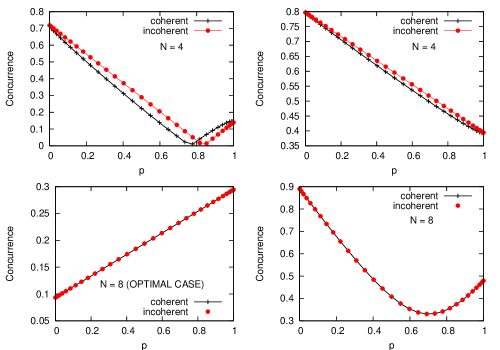
Figure 1: Concurrence of the first two qubits vs $p_{1}=\cos^{2}(\theta)$ for the superposition of two states ($k=2$) with $N=4$ and $N=8$ (see Eq. (28)) for two different realizations (left and right columns). The incoherent case is obtained on neglecting the interference terms in the superposition as in Eq. (32). The bottom left panel shows a case of optimality.

To estimate the typical value of $\mu_{1}$ and $\mu_{2}$ consider the Hilbert space of each entangled pair consisting of two qubits and take for the distribution of the coefficients the uniform or Haar measure of Eq. (15). The averages of $\mu_{1}$ and $\mu_{2}$ are both zero in this ensemble. However the second moments are nonzero and can be shown to be

$$\langle\mu_{1}^{2}\rangle=4^{-N},\;\;\;\langle\mu_{2}^{2}\rangle=4^{-(N-1)}.$$

This follows on observing that $\mu_{1}$ and $\mu_{2}$ in Eqs. (29, 31) are $N$ and $N-1$ fold products of inner-products of two four-vectors. Consider one such (square of the) inner-product and its ensemble average, the average being over the distribution where each of the 4-vectors, here denoted simply as $x_{i}$ and $y_{i}$ are distributed according to the measure in Eq. (15):

$$\left\langle\left(\sum_{i=1}^{4}x_{i}y_{i}\right)^{2}\right\rangle=\sum_{i=1}^{4}\left\langle x_{i}^{2}y_{i}^{2}\right\rangle=1/4.$$ (33)

The first equality follows as the odd powers average to zero, and the second equality follows as the ensemble average of each of the $x_{i}^{2}$ is $1/4$, which follows most easily from normalization.

Thus $\mu_{1}$ and $\mu_{2}$ are typically of the order of $2^{-N}$ and $2^{-(N-1)}$ respectively. In practice for most states with $N>8$ it is difficult to distinguish whether the incoherent two-qubit state $\rho$ obtained on dropping the interference term as in Eq. (32) is used or the actual reduced density matrix $\rho_{12}$ (Eq. (30)) is used. This is illustrated in Fig. (1), where random realizations of the two-qubit states $|\phi_{j}^{i}\rangle$ are used in Eq. (28) with $k=2$. Two such realizations are selected for the cases of $N=4$ and $N=8$ and the concurrence in the reduced density matrix of the first two qubits are calculated based on the exact state $\rho_{12}$ (Eq. (30), referred to in the figure as “coherent”) and the approximation $\rho$ (Eq. (32), referred to in the figure as “incoherent”). The concurrences are plotted as a function of the mixing between the states that are superposed in Eq. (28). It is seen from the figure that when $N=8$ whatever difference persist between the entanglement in $\rho$ and $\rho_{12}$ is not visible, while it is for $N=4$. Also from the $N=8$ case, the realization on the right, illustrates the convexity of concurrence as at $p=0,1$ two different two-qubit pure states are obtained while for intermediate $p$, the density matrix is an incoherent superposition of these (see Eq. (32)). However for $N=8$ the realization on the left is peculiar in that the concurrence for the intermediate values of $p$ is just a linear interpolation of the concurrences of the pure states. In this case one has hit upon what is studied in this paper as an optimal pair of pure states.

The approximate form of the reduced density matrix in Eq.(32) obtained by using the incoherent superposition condition holds also for complex states, however optimality results arise in the case of real state as studied in detail in the previous section. For $k>2$ similar considerations give rise to states of the form as in Eq. (1) where $p_{i}$ are equal to $|a_{i}|^{2}$. In terms of dimerized states, we see that superposing two of them leads to pairs of qubits that were originally entangled with each other retaining much of it. About $28.5\%$ of pairs of qubits would have simply the weighted entanglements of the states before superposition. On the other hand superposing three dimerized states leads to a significant decrease in the fraction of robust dimers, which is now $5.12\%$, and superposing more than three, the entanglement of a pair is bound to be smaller than the weighted entanglements.

IV Discussions and Summary

This work has used a particular measure of entanglement of two-qubit density matrices, namely concurrence, and studied questions of optimality, as defined herein, mainly restricting to the space of real states. Concurrence is only one measure of entanglement, but the entanglement of formation being a monotonic function of it renders it rather unique and as such this measure has been used in very many studies. What exactly the issue of optimality says about the geometry of the quantum space of states ZyckBook is an interesting question that is not pursued here. It may also be interesting to study other measures of non-classical correlation, such as discord ZurekDiscord from this perspective.

One possible application of optimality was discussed in the superposition of dimerized states. Such states are found in many quantum spin systems, such as the Majumdar Ghosh hamiltonian MajGhosh , and superpositions are relevant in the neighborhood of avoided crossings where it is known that interesting transformations of entanglement occur KarthikAudityaArul . Results not shown here indicate circumstances under which such intra-dimer entanglement can be broken if a dimerized state is superposed with a non-dimerized, completely random state. In particular this results in dimer density matrices being very close to Werner states Werner and therefore results in the entanglement of dimers vanishing when the random state component is more than $2/3$. In general the effect of superposition on entanglement has been studied vigorously Linden , as well as entanglement in the RVB states has been explored RVB . The results discussed in this paper may add in some small measure to the understanding of entanglement in such contexts.

Real states are often obtained as eigenstates of time-reversal symmetric systems and the discussion here will be of relevance to such systems, for instance to spin chains that have time-reversal. Clearly when the states are complex the above approach to finding optimality conditions does not work. In the case when $k=2$ the optimality condition is found to be the same as that for real states, namely $0<r_{11}r_{22}/r_{12}^{2}<1$ (except now $r_{12}$ is not restricted to the reals). Thus it is conceivable that as this is the unit interval in the complex plane, the measure of optimal states is zero. However of course, there could be an infinity of these, for instance all real states are possible candidates.

*

Appendix A Evaluation of an integral for the optimal fraction $f_{2}$

To recall, the integral is

$$f_{2}=\int\Theta(r_{11}r_{22})\Theta(r_{12}^{2}-r_{11}r_{22})P(\{x_{i}\})P(\{y_{i}\})\prod_{i=1}^{4}dx_{i}dy_{i},$$ (34)

where $r_{ij}=\langle\psi_{i}|\sigma_{y}\otimes\sigma_{y}|\psi_{j}\rangle$ , $|\psi_{i}\rangle$, $=1,2$ are two real and normalized 4-vectors, and the measures $P$ are the uniform measures in Eq. (15). First, the particular Pauli matrix $\sigma_{y}$ that appears can be replaced by the other Pauli matrices. In particular the $\sigma_{z}$ matrix being diagonal, offers a simpler look. This replacement is quite easily seen to be equivalent to some $45^{\circ}$ rotations of the original variables.

Also dropping the constraint on the product $r_{11}r_{22}$ will be useful. If the resultant integral is denoted as $f$, then it is shown below that $f_{2}$ is simply $f-1/2$. Next, it is proven that as far as $f$ is concerned, the two 4-vectors can be taken to be orthogonal. Decompose say $|\psi_{2}\rangle$ along the vector $|\psi_{1}\rangle$ and one orthogonal to it:

$$|\psi_{2}\rangle=\cos(\theta)|\psi_{1}\rangle+\sin(\theta)|\eta\rangle,$$ (35)

where $\langle\eta|\psi_{1}\rangle=0$. No additional phases are involved as the states are all real. A straightforward calculation shows that

$$r_{12}^{2}-r_{11}r_{22}=\sin^{2}(\theta)\left(\langle\psi_{1}|\sigma_{z}\otimes\sigma_{z}|\eta\rangle^{2}-\langle\eta|\sigma_{z}\otimes\sigma_{z}|\eta\rangle\langle\psi_{1}|\sigma_{z}\otimes\sigma_{z}|\psi_{1}\rangle\right).$$ (36)

The quantity within the brackets is precisely the same combination as in the L.H.S., except that instead of $|\psi_{i}\rangle$, the vectors are orthogonal. As $\sin^{2}(\theta)$ has a constant positive sign, this proves that we can consider the pairs, to begin with, as being orthogonal. In other words the sign of the combination $r_{12}^{2}-r_{11}r_{22}$ is invariant under the Gram-Schmidt orthogonalization process.

The additional constraint of the vectors being orthonormal introduces an additional Dirac delta function term in the measure. Writing the fraction $f$ as a ratio $f_{n}/f_{d}$, the numerator $f_{n}$ and the denominator $f_{d}$ are given by

$$f_{n}=\dfrac{8}{\pi^{2}}\int\Theta\left(r_{12}^{2}-r_{11}r_{22}\right)\delta\left(\sum_{i}x_{i}y_{i}\right)\delta\left(\sum_{i}x_{i}^{2}-1\right)\delta\left(\sum_{i}y_{i}^{2}-1\right)dx\,dy,$$ (37)

and

$$f_{d}=\dfrac{8}{\pi^{2}}\int\delta\left(\sum_{i}x_{i}y_{i}\right)\delta\left(\sum_{i}x_{i}^{2}-1\right)\delta\left(\sum_{i}y_{i}^{2}-1\right)dx\,dy.$$ (38)

All the sums are from $1$ to $4$ and $dx\,dy$ is the Euclidean eight dimensional volume element. The factor $8/\pi^{2}$ is introduced for later convenience alone. To be further explicit the combination $r_{12}^{2}-r_{11}r_{22}=$

$$\left(x_{1}y_{1}-x_{2}y_{2}-x_{3}y_{3}+x_{4}y_{4}\right)^{2}-(x_{1}^{2}-x_{2}^{2}-x_{3}^{2}+x_{4}^{2})(y_{1}^{2}-y_{2}^{2}-y_{3}^{2}+y_{4}^{2}).$$ (39)

Introducing a series of transformation to various two-dimensional polar coordinates (in the ($x_{1},x_{4}$) pair, the $(x_{2},x_{3})$ pair, etc., as well as in the resulting radii) and performing two delta function integrals corresponding to the normalizations results is:

$$\begin{split}f_{n}=2\int\Theta\left[\left(\cos(\alpha)\cos(\beta)\cos(\theta)-\sin(\alpha)\sin(\beta)\cos(\phi)\right)^{2}-\cos(2\alpha)\cos(2\beta)\right]\\ \delta\left[\cos(\alpha)\cos(\beta)\cos(\theta)+\sin(\alpha)\sin(\beta)\cos(\phi)\right]\sin(2\alpha)\sin(2\beta)d\alpha d\beta d\theta d\phi,\end{split}$$ (40)

and a corresponding integral for $f_{d}$, only without the Heaviside theta function constraint. Here $\alpha,\beta\in[0,\pi/2]$ while $\theta,\phi\in[0,2\pi]$. As a check, the integral can be easily done without either the Heaviside theta or the Dirac delta functions to give $8\pi^{2}$, which is exactly the factor that follows from the normalization of the two Dirac delta normalization constraints; see Eq. (15), if one takes into account the factor $8/\pi^{2}$ that is introduced in Eq. (37).

Introducing variables $v$ and $u$ as $\cos(\alpha)\cos(\beta)\cos(\theta)\pm\sin(\alpha)\sin(\beta)\cos(\phi)$ respectively, allows the delta function integration over the $v$ variable to be performed and results in:

$$f_{n}=\int\dfrac{\Theta\left(u^{2}-\cos(2\alpha)\cos(2\beta)\right)\,du\,d\alpha\,d\beta}{\sqrt{1-\dfrac{u^{2}}{4\cos^{2}(\alpha)\cos^{2}(\beta)}}\sqrt{1-\dfrac{u^{2}}{4\sin^{2}(\alpha)\sin^{2}(\beta)}}}.$$ (41)

Notice that the given range of $\alpha$ and $\beta$, $[0,\pi/2]^{2}$ can be divided into four equal squares, such that the $\Theta$ function constraint is effective only in $[0,\pi/4]^{2}$ and in $[\pi/4,\pi/2]^{2}$, as $\cos(2\alpha)\cos(2\beta)$ is negative elsewhere. The range of the $u$ integration is restricted depending on $\alpha,\beta$. Taking the range $[0,\pi/4]$, the contribution from it is denoted $f_{n}^{ll}$, $ll$ for lower-lower, we have:

$$f_{n}^{ll}=\int_{0}^{\pi/4}d\alpha\int_{\beta_{0}}^{\pi/4}d\beta\int_{u_{0}}^{u_{1}}\dfrac{du}{\sqrt{1-\dfrac{u^{2}}{4c_{\alpha}^{2}c_{\beta}^{2}}}\sqrt{1-\dfrac{u^{2}}{4s_{\alpha}^{2}s_{\beta}^{2}}}},$$ (42)

where

$$\beta_{0}=\sin^{-1}\sqrt{1/2-s_{\alpha}^{2}},\;u_{0}=\sqrt{c_{2\alpha}c_{2\beta}},\;\mbox{and}\;u_{1}=2s_{\alpha}s_{\beta},$$

and $s_{\alpha}$ stands for $\sin(\alpha)$ etc.. The limits of the integration are such that the $\Theta$ function constraint is satisfied as well as the square-roots are real numbers. The denominator fraction can be similarly split up, and in fact $f_{d}^{ll}$ differs from the above in that $\beta_{0}=0$ as well as $u_{0}=0$. It is also not hard to see that $f_{n}^{uu}$ ($uu$ for upper-upper) is same as $f_{n}^{ll}$ and similarly for $f_{d}$. In the other two regions, as the constraint is not operational, and because of symmetry, it follows that: $f_{d}^{ul}=f_{d}^{lu}=f_{n}^{ul}=f_{n}^{lu}\equiv f^{ul}$. It then follows that

$$f=\dfrac{2f^{ul}+2f_{n}^{ll}}{2f^{ul}+2f_{d}^{ll}}.$$ (43)

An evaluation of the three corresponding integrals is carried out numerically and results in $f_{n}^{ll}=0.116850...$, $f^{ul}=1/2$, $f_{d}^{ll}=0.285391...$. It is remarked that standard softwares could not evaluate the integrals symbolically, however the numerical results are sufficient to give the fraction $f=0.785398...$, which is $\pi/4$ to 1 part in $10^{6}$. It is also easy to similarly see that $f_{d}^{ll}=(\pi-2)/4$ and from consistency$f_{n}^{ll}=(\pi^{2}-8)/16$.

Returning to the integral in Eq. (34) for the fraction $f_{2}$ we see that there are two $\Theta$ constraints, while we have considered only one, namely the second one. If the first constraint $\Theta(r_{11}r_{22})$ alone is present, it is easy to see that the integral is $1/2$. This also follows from the fact that $r_{11}$ and $r_{22}$ are both independent and uniformly distributed. We also state parenthetically without proof that $r_{12}$ is distributed according to the semi-circle distribution. Now, if $r_{11}r_{22}$ is negative, then surely $r_{12}^{2}-r_{11}r_{22}$ is positive, which is $50\%$ of the time. Thus the fraction of cases when $r_{11}r_{22}$ is positive and $r_{12}^{2}-r_{11}r_{22}$ is positive is $f-1/2$, which is precisely the required fraction $f_{2}$. Thus we have evaluated $f_{2}$ and presented sufficient evidence that it is actually $(\pi-2)/4$. It is not clear if it is only a coincidence that this is also precisely $f_{d}^{ll}$. The evaluation presented here may, by far, not be the “optimal” one, but is the best the authors could come up with.

References

- (1) R. Horodecki, P. Horodecki, M. Horodecki and K. Horodecki, Rev. Mod. Phys. 81, 865 (2009).
- (2) S. Hill and W. K. Wootters, Phys. Rev. Lett. 78, 5022 (1997); W. K. Wootters, Phys. Rev. Lett. 80, 2245 (1998).
- (3) M. A. Nielsen and I. L. Chuang, Quantum Computation and Quantum Information (Cambridge Univ. Press, 2000 Cambridge).
- (4) A. Osterloh, Luigi Amico, G. Falci, and Rosario Fazio, Nature 416, 608 (2002).
- (5) D. Bruß, Phys. Rev. A 60, 4344 (1999).
- (6) V. M. Kendon, Kae Nemoto, and W. J. Munro, J. Mod. Opt. 49, 1709 (2002).
- (7) A. J. Scott and C. M. Caves, J. Phys. A: Math. Gen. 36, 9553 (2003).
- (8) A. Uhlmann, Phys. Rev. A 62, 032307 (2000).
- (9) Noah Linden, Sandu Popescu and John A. Smolin, Phys. Rev. Lett. 97, 100502 (2006).
- (10) J. Nisert, N. J. Cerf, Phys. Rev. A 74, 042328 (2007).
- (11) Chang-shui Yu, X. X. Yi, and He-shan Song, Phys. Rev. A 75, 022332 (2007).
- (12) Yong-Cheng Ou, Heng Fan, Phys. Rev. A 76, 022320 (2007).
- (13) Gilad Gour, Aidan Roy, Phys. Rev. A 77, 012336 (2008).
- (14) Wei Song, Nai-Le Liu and Zeng-Bing Chen, Phys. Rev. A 76, 054303 (2007).
- (15) Andreas Osterloh, Jens Siewert and Armin Uhlmann, Phys. Rev. A 77, 032310 (2008).
- (16) T. A. Brody, J. Flores, J. B. French, P. A. Mello, A. Pandey and S. S. Wong, Rev. Mod. Phys. 53, 385 (1981).
- (17) C. M. Caves, C. A. Fuchs and P. Rungta, Found. Phys. Lett. 14, 199 (2001).
- (18) P. W. Anderson, G. Baskaran, Z. Zou, and T. Hsu, Phys. Rev. Lett. 58, 2790 (1987).
- (19) I. Bengtsson and K. Zyczkowski, Geometry of Quantum States: An Introduction to Quantum Entanglement (Cambridge University, Cambridge, England, 2007).
- (20) H. Ollivier and W. H. Zurek, Phys. Rev. Lett. 88, 017901 (2001).
- (21) C. K. Majumdar and D. P. Ghosh, J. Math. Phys. 10, 1388 (1969); J. Math. Phys. 10, 1399 (1969).
- (22) J. Karthik, A. Sharma, and A. Lakshminarayan, Phys. Rev. A 75, 022304 (2007).
- (23) R. F. Werner, Phys. Rev. A 40, 4277 (1989).
- (24) Anushya Chandran, Dagomir Kaszlikowski, Aditi Sen(De), Ujjwal Sen, and Vlatko Vedral, Phys. Rev. Lett. 99, 170502 (2007); Ravishankar Ramanathan, Dagomir Kaszlikowski, Marcin Wiesniak, and Vlatko Vedral, Phys. Rev. B 78, 224513 (2008).