Correcting errors in a quantum gate with pushed ions via optimal control

Abstract

We analyze in detail the so-called “pushing gate” for trapped ions, introducing a time dependent harmonic approximation for the external motion. We show how to extract the average fidelity for the gate from the resulting semi-classical simulations. We characterize and quantify precisely all types of errors coming from the quantum dynamics and reveal for the first time that slight nonlinearities in the ion-pushing force can have a dramatic effect on the adiabaticity of gate operation. By means of quantum optimal control techniques, we show how to suppress each of the resulting gate errors in order to reach a high fidelity compatible with scalable fault-tolerant quantum computing.

I Introduction

Trapped ultracold ions have represented a major candidate for the implementation of scalable quantum information processing since the beginning of this research field. The first proposal of an ion-based quantum computer by Cirac and Zoller in 1995 Cirac and Zoller (1995) has been followed by a great variety of other schemes based on ions Cirac and Zoller (2000), on other quantum optical systems like neutral atoms Jaksch et al. (1999); Calarco et al. (2000) and on solid-state systems Burkard et al. (1999) as well. With the progress of experimental techniques and the demonstration of entangling quantum gates based on several different candidate physical systems, the focus has progressively shifted toward the fulfilment of scalability desiderata DiVincenzo (2000), that is, the realization of quantum gates with very high fidelities, in the range 0.999 – 0.9999.

Gate errors in a real implementation of a given quantum gate scheme can be reduced by different means. Some errors arise from (or are increased by) experimental imprecisions of a technical nature and can be controlled by careful alignment, stabilization etc. of the experimental apparatus. Other errors stem from unaviodable interactions with the environment and can be reduced by simply completing the gate in as short a time as possible. Typically, a gate scheme can be made faster by simple scaling to higher intensities, shorter distances etc. If such simple optimizations of the gate prove insufficient, one needs to consider changes to the scheme itself and trade simplicity for improved performance. This is exactly the goal of quantum optimal control techniques D’Alessandro (2008) which allow for a precise tailoring of the system’s evolution by time-dependent tuning of some external parameters. With sufficient control over these parameters, a given target state can often be reached with minimal errors even over short gate operation times. The application of these methods to quantum information systems requires in turn a very accurate simulation of the dynamics and a careful understanding of the targeted error sources. This is precisely the aim of this paper, in the specific case of the two-qubit ion gate first proposed in Cirac and Zoller (2000) and subsequently analyzed in Calarco et al. (2001); Šašura and Steane (2003). In this “pushing gate” the qubits are encoded in the internal states of two ions. Each ion is held in a separate microtrap and state-selective “push” potentials are applied in order to modify the distance and thus the Coulomb interaction between ions, see Sec. III below. We shall first point out a series of issues that arise when the assumption of spatial homogeneity of the ion-driving force is dropped, and subsequently develop a way to correct each of these issues, exploting a range of ideas, including in a crucial way optimal control methods.

It should be noted from the outset that in the present paper, we analyze the pushing gate without what is called the $\pi$-pulse method in Refs. Calarco et al. (2001); Šašura and Steane (2003), where it was shown to dramatically reduce some types of errors. The $\pi$-pulse method is a spin-echo technique and requires the gate to be repeated with the internal state of the ions flipped. Typically, single particle operations like flipping the internal states can be done with high fidelity, and it is reasonable to expect that eventually the $\pi$-pulse method will be used. However, internal state control is at least in principle a separate issue from the pushing gate operation itself. Keeping the design process modular in spirit, it is relevant to optimize the gate without this additional trick and thus pave an alternative road to high fidelities. As will become clear below, we extract quite general noise reduction methods from the automated numerical optimization results and it is an interesting topic for future research to combine these with the $\pi$-pulse method.

The remainder of the paper is organized as follows. In Sec. II we introduce the general setting of conditional dynamics gate schemes, a useful approximation for simulating such a gate, and a measure of the gate errors. In Sec. III we specialize to the pushing gate. The un-optimized performance of the gate is reported in Sec. IV and in Sec. V we show how this performance can be significantly improved by a combination of “manual” changes and numerical optimal control methods. Finally we conclude in Sec. VI. The Appendix contains a number of more technical results and derivations.

II Conditional dynamics

The basic idea of the so-called pushing gate is one of conditional dynamics, i.e. we apply potentials depending on the internal state of the two ions. The internal states themselves are not changed during the gate, or, in the case of the $\pi$-pulse method, are changed on a much shorter time-scale than the external dynamics. This means that the analysis of the problem splits into four separate evolutions for the external state, one for each of the logical (internal) states, $00$, $01$, $10$, and $11$. In the following, these four evolutions will be denoted “branches” and will be indexed by $\beta\in\{00,01,10,11\}$. The complete Hamiltonian can be written in the form of a sum of internal$\otimes$external factorized terms

$$\hat{H}^{\text{tot}}(t)=\sum_{\beta}|\beta\rangle\!\langle\beta|\otimes\hat{H}^{\text{ex}}_{\beta}(t)$$ (1)

and it results in an evolution operator of a similar form

$$\hat{U}^{\text{tot}}(t)=\sum_{\beta}|\beta\rangle\!\langle\beta|\otimes\hat{U}_{\beta}^{\text{ex}}(t).$$ (2)

Ideally, when $t=T$ at the end of the gate, the $U_{\beta}^{\text{ex}}$ should differ from each other by at most a phase factor multiplying a common unitary operator $\hat{U}^{\text{ex}}_{\text{com}}$

$$\hat{U}^{\text{ex}}_{\beta}(T)=e^{i\theta_{\beta}}\hat{U}^{\text{ex}}_{\text{com}}$$ (3)

so that $\hat{U}^{\text{tot}}$ itself can be factorized:

$$\hat{U}^{\text{tot}}(T)=\left(\sum_{\beta}|\beta\rangle\!\langle\beta|e^{i\phi_{\beta}}\right)\otimes\hat{U}^{\text{ex}}_{\text{com}}.$$ (4)

The internal evolution is then that of a phase gate, while the external evolution can in principle be undone using internal-state independent potentials.

The requirement (3) is very hard to achieve and would make the gate completely independent on the initial external state. However, we can typically assume to have some degree of control over the initial external state, e.g. by cooling the particles before the gate. This means that (3) need only hold when restricted to a subset of the complete Hilbert space, typically the states of relatively low energy. In Appendix B we show how to evaluate the performance of the gate in general. For now, we note that since only the low energy part of $\hat{U}^{\text{ex}}_{\beta}(T)$ will be important, we can focus on getting a good approximation for this part when trying to simulate the gate dynamics.

A low initial energy means particles localized near the potential minimum and this suggests using a harmonic approximation to the real potential . The simplest choice is to Taylor expand around a fixed point, which is not changed during the gate operation. The next level of refinement is to expand around the instantaneous potential minimum. This works very well if the gate operation is nearly adiabatic so the particles stay near the (moving) minimum at all times. However, it may be desirable to make fast and substantial changes to the potential during the gate and that may induce pronounced non-adiabatic dynamics. In that case, the harmonic approximation can still be a good one provided it is done around the classical trajectories of the particles. Typically these trajectories cannot be computed analytically, but for any moderate number of particles it is a numerically simple task to find them. Below we will use this method and show how it leads to a relatively simple characterization of $U^{\text{ex}}_{\beta}$.

II.1 Harmonic approximation

In this section we focus on a single branch of the evolution and thus suppress the $\beta$ index. Let us denote by $\mathbf{\overline{x}}(t)$ the classical trajectory, which is found by solving classical equations of motion. The time-dependent, second order Taylor expansion of the potential $V(t,\mathbf{x})$ around $\mathbf{\overline{x}}(t)$ reads simply

$$V_{\text{so}}(t,\mathbf{x})=V^{(0)}(t)+\Delta\mathbf{x}^{\mathrm{T}}\mathbf{V}^{(1)}(t)+\frac{1}{2}\Delta\mathbf{x}^{\mathrm{T}}V^{(2)}(t)\Delta\mathbf{x},$$ (5)

with $\Delta\mathbf{x}=\left[\mathbf{x}-\mathbf{\overline{x}}(t)\right]$ and

$$\begin{split}V^{(0)}(t)&=V(t,\mathbf{\overline{x}}),\\ V^{(1)}_{i}(t)&=\frac{\partial V}{\partial x_{i}}(t,\mathbf{\overline{x}}),\\ V^{(2)}_{ij}(t)&=\frac{\partial^{2}V}{\partial x_{i}\partial x_{j}}(t,\mathbf{\overline{x}}).\end{split}$$ (6)

Note that we will still use $\mathbf{x}$ as our coordinate, i.e. we are not changing to a coordinate system moving with $\mathbf{\overline{x}}(t)$, we simply use a potential that approximates the real potential close to $\mathbf{\overline{x}}(t)$. Collecting terms of equal order in $\mathbf{x}$ leads to the alternative form

$$V_{\text{so}}(t,\mathbf{x})=E(t)-\mathbf{x}^{\mathrm{T}}\mathbf{F}(t)+\frac{1}{2}\mathbf{x}^{\mathrm{T}}K(t)\mathbf{x},$$ (7)

with

$$\begin{split}E(t)&=V^{(0)}(t)-\mathbf{\overline{x}}^{\mathrm{T}}(t)\mathbf{V}^{(1)}(t)+\frac{1}{2}\mathbf{\overline{x}}^{\mathrm{T}}(t)V^{(2)}(t)\mathbf{\overline{x}}(t),\\ \mathbf{F}(t)&=-\mathbf{V}^{(1)}(t)+{V}^{(2)}(t)\mathbf{\overline{x}}(t),\\ {K}(t)&={V}^{(2)}(t).\end{split}$$ (8)

II.2 Gaussian evolution

The big advantage of choosing a second order approximation to the real potential is that this restricts the corresponding approximate $\hat{U}^{\text{ex}}(t)$ to be Gaussian for all $t$. Let us introduce the compact notation $\mathbf{q}=(\mathbf{x},\mathbf{p})$ and define the matrix $J$ by

$$J=\begin{bmatrix}0&\mathbb{I}_{n}\\ -\mathbb{I}_{n}&0\end{bmatrix},$$ (9)

where $n$ is the number of degrees of freedom. Then the usual canonical commutation relations can be written as

$$[q_{i},q_{j}]=iJ_{ij}.$$ (10)

With the potential of Eq. (7) and a matrix of particle masses $M=\text{diag}(m_{1},\ldots,m_{n})$ the time-dependent Hamiltonian becomes

$$\hat{H}_{\text{so}}=\frac{1}{2}\hat{\mathbf{p}}^{\mathrm{T}}M^{-1}\hat{\mathbf{p}}+V_{\text{so}}(t,\hat{\mathbf{x}}).$$ (11)

In Appendix A we show that such a Hamiltonian leads to an evolution operator of the form

$$\hat{U}(t)=e^{-i\phi(t)}\hat{D}_{\mathbf{c}(t)}\hat{W}_{b(t)},$$ (12)

where $\hat{D}_{\mathbf{c}}$ is a displacement operator and $\hat{W}_{b}$ a squeezing operator

$$\begin{split}\hat{D}_{\mathbf{c}}&=e^{-i\mathbf{\mathbf{c}}^{\mathrm{T}}J\hat{\mathbf{q}}}\\ \hat{W}_{b}&=e^{-i\frac{1}{2}\hat{\mathbf{q}}^{\mathrm{T}}b\hat{\mathbf{q}}}.\end{split}$$ (13)

The scalar $\phi$, the vector $\mathbf{c}$, and the matrix $S=\exp(Jb)$ should satisfy the following equations of motion:

$$\begin{split}\frac{\partial}{\partial t}\phi&=E-\frac{1}{2}\mathbf{F}^{\mathrm{T}}\mathbf{\overline{x}},\\ \frac{\partial}{\partial t}\mathbf{c}&=Jh\mathbf{c}+\begin{bmatrix}0\\ \mathbf{F}\end{bmatrix},\\ \frac{\partial}{\partial t}S&=JhS,\end{split}$$ (14)

where the $2n\times 2n$ matrix $h$ is defined by

$$h(t)=\begin{bmatrix}K(t)&0\\ 0&M^{-1}\end{bmatrix}.$$ (15)

The form of solution (12)–(14) holds for any second order Hamiltonian. In the particular case where $V_{\text{so}}$ is a Taylor expansion of a real potential around the classical trajectory $\mathbf{\overline{x}}(t)$, the equation of motion for $\mathbf{c}$ reduces to the exact equation of motion for $\mathbf{\overline{q}}=(\mathbf{\overline{x}},\mathbf{\overline{p}})$ where $\mathbf{\overline{p}}$ is the classical momentum. In the following, we will therefore write $\mathbf{\overline{q}}$ instead of $\mathbf{c}$. It is then important to remember that the right-hand sides of Eqs. (14) are in general non-linear functions of $\mathbf{\overline{x}}$.

II.3 Fidelity

We can quantify the performance of the gate by calculating the average fidelity $F_{\mathrm{avg}}$ (see Appendix B) between the obtained output state and the ideal one when the input state is varied. One can then separate out three kinds of contributions to the deviation of $F_{\mathrm{avg}}$ from 1 (the perfect gate)

$$1-F_{\mathrm{avg}}=\mathrm{E}_{\theta}+\mathrm{E}_{\mathbf{\overline{q}}}+\mathrm{E}_{S}$$ (16)

The three types of errors each have their physical interpretation. The most straightforward one pertains to the sloshing errors $\mathrm{E}_{\mathbf{\overline{q}}}$ which correspond to a residual motion of the ions after the gate has been completed and the micro-traps are again at rest. The phase errors $\mathrm{E}_{\theta}$ are errors in the gate phase. Finally, the breathing errors $\mathrm{E}_{S}$ are induced by differences in the harmonic approximation parameters around the classical trajectory for different internal states. For example, in the case we consider, when the particles are pushed closer together, the second order term in the Coulomb repulsion becomes larger, cf. Eq. (25) below.

In our model we assume that systematic, local phase errors can be undone. Then an explicit calculation in Appendix B, shows that the phase errors are given by

$$\mathrm{E}_{\theta}=\frac{1}{20}\left(\theta_{00}-\theta_{01}-\theta_{10}+\theta_{11}-\pi\right)^{2}$$ (17)

with $\theta_{\beta}=-\phi_{\beta}+\text{Tr}[b_{\beta}\gamma]$, where $\gamma$ is the covariance matrix of the external state, see Section B.3 of the Appendix. Note the inclusion of the $\text{Tr}[b_{\beta}\gamma]$ terms in the definition of $\theta_{\beta}$: These terms correspond to phase contributions from average excitation energy in the traps and are therefore temperature dependent through $\gamma$. For our parameters they are small.

The sloshing errors are given by

$$\mathrm{E}_{\mathbf{\overline{q}}}=\frac{1}{20}\sum_{\alpha<\beta}(\mathbf{\overline{q}}_{\alpha}-\mathbf{\overline{q}}_{\beta})^{\mathrm{T}}\gamma(\mathbf{\overline{q}}_{\alpha}-\mathbf{\overline{q}}_{\beta}),$$ (18)

and the breathing errors are

$$\begin{split}\mathrm{E}_{S}=&\frac{1}{40}\sum_{\alpha<\beta}\text{Tr}\left[(b_{\alpha}-b_{\beta})\gamma(b_{\alpha}-b_{\beta})\gamma\right]\\ &+\frac{1}{160}\sum_{\alpha<\beta}\text{Tr}\left[(b_{\alpha}-b_{\beta})J(b_{\alpha}-b_{\beta})J\right].\end{split}$$ (19)

Here $\phi_{\beta}$, $\mathbf{\overline{q}}_{\beta}$, and $b_{\beta}$ are defined in Eqs. (12,13), and are the variables describing the Gaussian approximation in the $\beta$ branch of the evolution. Again $\gamma$ introduce temperature dependence.

III The pushing gate

Let us now focus on the particular case of the pushing gate. Here we have two ions, each in a separate micro-trap . To further simplify the discussion, we concentrate on just one spatial dimension, i.e. there are two degrees of freedom, $n=2$. The ions are assumed to be of identical mass, $m_{1}=m_{2}=m$, and thus $M=m\mathbb{I}_{2}$. The potential energy consists of a micro-trap for each ion, time- and internal state-dependent pushing potentials, and the Coulomb interaction. The pushing potentials can be realised as optical dipole potentials generated by focused laser beams. The time-dependence of these potentials is most easily achieved by controlling the intensity of the laser and the state-selectivity by polarization selection rules Šašura and Steane (2003). We assume that the form for the internal state labeled by $\beta$ is

$$\begin{split}V^{(\beta)}(t,\mathbf{x})=&\sum_{i=1,2}\frac{1}{2}m\omega^{2}x_{i}^{2}+\frac{e^{2}}{4\pi\epsilon_{0}\left|d+x_{2}-x_{1}\right|}\\ &+\sum_{i=1,2}f_{i}^{(\beta)}(t)\frac{\hbar\omega}{a_{0}}\left[-(-1)^{i}x_{i}+\frac{G}{a_{0}}x_{i}^{2}\right].\end{split}$$ (20)

The trapping potentials are assumed to be perfectly harmonic. The state-dependent pushing amplitudes $f^{(\beta)}_{i}$ are such that the ions are only pushed if they are in the internal state 1, $f^{(\beta)}_{i}(t)=\delta_{\beta_{i},1}f(t)$. Note that the $(-1)^{i}$ factor means that ion 1 is pushed to the left and ion 2 to the right. Non-linear contributions to the pushing potentials are included via the constant $G$. The harmonic oscillator ground state size is $a_{0}=\sqrt{\hbar/m\omega}$. The two coordinates $x_{1}$ and $x_{2}$ are taken to have origin in the respective trap centers, a distance $d$ apart. Experimentally, the parameters in (20) can be varied quite a lot (see e.g. Šašura and Steane (2003)). Trap distances $d$ from $100\mu m$ all the way down to $1\mu m$ are within technological reach. The trap frequency $\omega$ can be chosen in the range $2\pi\times 10^{4}-10^{7}\mathrm{Hz}$ which for e.g. Ca⁺ ions will mean an oscillator length $a$ from $150\mathrm{nm}$ down to $5\mathrm{nm}$.

It should be noted that the use of optical dipole potentials to generate the state selective pushing forces will in general introduce large single qubit phases due to ac-Stark shifts. This is not a problem as such, but it means that even small fluctuations in laser intensities will lead to loss of gate fidelity. For the particular case of the pushing gate, the ac-Stark shifts can be balanced against the Coulomb energy as discussed in Ref. Šašura and Steane (2003). Obviously ac-Stark shifts are common to many gate proposals that uses optical potentials. An experimentally demanding, but quite general solution is to compensate the shifts along the lines of Refs. Häffner et al. (2003); Kaplan et al. (2002). In the present work, we focus on errors that are more directly related to the motion of the ions and assume that the push potentials are effectively non-fluctuating.

.

III.1 Dimensionless Hamiltonian

The relative strength of the Coulomb interaction to the trapping potentials turns out to be conveniently quantified by

$$\epsilon=\frac{\frac{e^{2}}{\pi\epsilon_{0}d}}{m\omega^{2}d^{2}}=\frac{a_{0}^{2}}{d^{2}}\frac{\frac{e^{2}}{\pi\epsilon_{0}d}}{\hbar\omega},$$ (21)

which is the ratio of the energy scale of the Coulomb and trap potential energies at the equilibrium positions of the ions. In Ref. Šašura and Steane (2003) it was found that $\epsilon\ll 1$ is the most promising regime. In oscillator units, the Hamiltonian for the branch labeled by $\beta$ reads

$$\begin{split}\hat{H}^{(\beta)}_{\text{push}}(t)=&\sum_{i=1,2}\frac{1}{2}\left[\hat{p}_{i}^{2}+\hat{x}_{i}^{2}\right]+\frac{\epsilon}{4}\frac{\frac{d^{2}}{a_{0}^{2}}}{\left|1+\frac{a_{0}}{d}\left(\hat{x}_{2}-\hat{x}_{1}\right)\right|}\\ &-\sum_{i=1,2}f^{(\beta)}_{i}(t)\left[\hat{x}_{i}+G\hat{x}_{i}^{2}\right].\end{split}$$ (22)

III.2 Harmonic approximation

When Eqs. (8) are specialized to the pushing gate, we get the following:

$$E^{(\beta)}(t) =\frac{1}{4}\epsilon\frac{a_{0}}{d}\left(\frac{\overline{x}_{2}^{(\beta)}-\overline{x}_{1}^{(\beta)}}{1+\frac{a_{0}}{d}\left(\overline{x}^{(\beta)}_{2}-\overline{x}_{1}^{(\beta)}\right)}\right)^{3}$$ (23)

$$F_{i}^{\beta)}(t) =-(-1)^{i}f_{i}^{(\beta)}(t)\mp\frac{1}{4}\epsilon\frac{d}{a_{0}}\frac{1+3\frac{a_{0}}{d}\left(\overline{x}_{2}^{(\beta)}-\overline{x}_{1}^{(\beta)}\right)}{\left[1+\frac{a_{0}}{d}\left(\overline{x}_{2}^{(\beta)}-\overline{x}_{1}^{(\beta)}\right)\right]^{3}}$$ (24)

$$\begin{split}K_{ii}^{(\beta)}(t)&=1+2f_{i}^{(\beta)}(t)G\\ &\phantom{=f_{i}}+\frac{1}{2}\epsilon\frac{1}{\left[1+\frac{a_{0}}{d}\left(\overline{x}_{2}^{(\beta)}-\overline{x}_{1}^{(\beta)}\right)\right]^{3}}\end{split}$$ (25)

$$\begin{split}K_{12}^{(\beta)}(t)&=K_{21}^{(\beta)}(t)=-\frac{1}{2}\epsilon\frac{1}{\left[1+\frac{a_{0}}{d}\left(\overline{x}_{2}^{(\beta)}-\overline{x}_{1}^{(\beta)}\right)\right]^{3}}.\end{split}$$ (26)

When these expressions are inserted into Eqs. (14) and (15) we are ready to simulate the gate.

IV Results of simulation

IV.1 Choice of parameters

Even with the simplifications we have introduced, there are still a lot of parameters in the problem. The optimal “working point” will always be dependent on experimental considerations beyond the simplified model treated here. For a discussion of parameters and design decisions, see Ref. Šašura and Steane (2003). For concreteness we have chosen to focus on a limited set of parameters. We first of all assume the individual ion traps to be very well separated and let $a/d=0.001$ in all calculations. Likewise, we assume a reasonably low value for $\epsilon$ of $0.04$. Such parameters would result from e.g. ⁴⁰Ca ions placed in micro-traps with trapping frequencies of $\omega\sim 2\pi\times 5\mathrm{MHz}$ and separated by a distance of $\sim 7\mu\mathrm{m}$. For a the traveling wave configuration with beam waist $w$ considered in Ref. Šašura and Steane (2003), $G=4(a/w)(w/2x_{0}-2x_{0}/w)$ where $x_{0}$ is the initial position of the ion relative to the beam center. For realistic focusing of the push beam, $w\sim 1\mu\mathrm{m}$ this suggests to vary the non-linearity coefficient $G$ between $0$ and $3\times 10^{-2}$. As the initial temporal shape of the push pulse we choose a Gaussian $f(t)=\xi\exp(-t^{2}/\tau^{2})$, where the amplitude $\xi$ should be chosen to give a gate phase of $\pi$. A simple estimate (for $G=0$) suggests that we choose Calarco et al. (2001)

$$\xi^{2}=\frac{\pi}{\sqrt{\pi/8}\;\epsilon\sqrt{1+\epsilon/2}\;\omega\tau}.$$ (27)

The temporal width of the pulse, $\tau$, should be within an order of magnitude from the trap period if we want a fast gate. We will mainly look at $\tau$ in the range 1 to 10 trap periods, which for the parameters quoted above results a maximum excursion due to the push in the range from 12$a_{0}$ down to 3$a_{0}$.

IV.2 Phase errors

The choice of push amplitude expressed by Eq. (27) is not optimal. This can be seen in Fig. 1 where we plot $\mathrm{E}_{\theta}$ as a function of $G$. Even for $G=0$ the gate phase is not exactly $\pi$. For $\omega\tau=3.5$ we see that a nonzero $G$ can improve the gate phase. This is not surprizing, but also not very useful as we shall see below that $\mathrm{E}_{\theta}$ is in general easy to reduce.

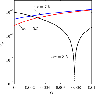
Figure 1: Phase errors with non-uniform pushing forces. The physical parameters are: $\epsilon=0.04$, $a/d=0.001$, and $\omega\tau=3.5$ (black), $5.5$ (red) and $7.5$ (blue). Results for temperatures of $T=0.125,1$ and $8\times\hbar\omega/k_{\mathrm{B}}$ are plotted for each value of $\tau$ and are indistinguishable from each other.

In Fig. 1 results for three different temperatures are plotted, but the dependence on temperature is completely negligible.

IV.3 Sloshing errors

Let us now turn to the errors described by the $\mathrm{E}_{\mathbf{\overline{q}}}$ term in Eq. (62), the sloshing errors. Fig. 2

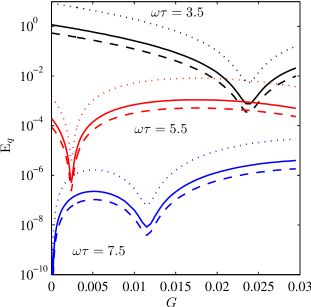
Figure 2: Sloshing errors with non-uniform pushing forces. The physical parameters are: $\epsilon=0.04$, $a/d=0.001$, and $\omega\tau=3.5$ (black), $5.5$ (red), and $7.5$ (blue). We plot $\mathrm{E}_{\mathbf{\overline{q}}}$ as a function of $G$. As explained in the text, there exist nonzero values of $G$ where the sloshing is strongly suppressed. Results for temperatures of $T=0.125$, 1 and $8\times\hbar\omega/k_{\mathrm{B}}$ are plotted as dashed, full and dotted lines, respectively.

shows how these errors are strongly dependent on $G$, the strength of the non-linearity of the pushing potential. A series of minima of $\mathrm{E}_{\mathbf{\overline{q}}}$ as a function $G$ can be seen. The optimal values of $G$ depends on the chosen duration of the pulse, $\tau$. Each minima is associated with the ions performing an integer number of “non-adiabatic oscillations” during the push pulse. This is illustrated in Fig. 3

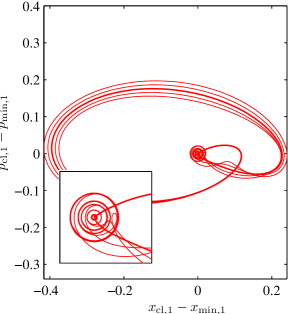
Figure 3: Phase-space trajectories for ion 1 for a push duration of $\omega\tau=5.5$. The coordinates are relative to the potential minimum in which ion 1 is trapped. Perfect adiabatic evolution would correspond to the ion simply following this minimum and thus the trajectory would be the single point $(0,0)$ in this plot. Since the push is not infinitely slow, the ion will first lag behind the moving minimum and then oscillate in the moving potential. When the potential minimum again approaches its original position, the ion may happen to have just the right position and speed in order to end up at rest. Whether this is the case depends (for fixed push pulse) on $G$: the higher $G$, the more the confinement is increased during the push. In the figure, the thick line corresponds to $G=0.002$, which is nearly optimal w.r.t. returning the ion to rest. The thin lines correspond to $G=0,0.001,0.003,0.004$. The lowest $G$ gives the outermost curve over the main part of the “loop” in the figure.

where the trajectory of ion 1 with respect to its trap minimum is plotted for values of $G$ that are below, at and above the one that leads to the lowest $\mathrm{E}_{\mathbf{\overline{q}}}$.

In contrast to $\mathrm{E}_{\theta}$ above, $\mathrm{E}_{\mathbf{\overline{q}}}$ depends noticeably on whether $T$ is $0.125$, $1$ or $8\times\hbar\omega/k_{\mathrm{B}}$. Higher temperatures always increase the sloshing errors and for $k_{\mathrm{B}}T/\hbar\omega\gg 1$ we find that $\mathrm{E}_{\mathbf{\overline{q}}}$ scales as $T$ since $\gamma$ does [see Eqs. (53) and (54)].

Curves for three different values of $\tau$ are plotted in Fig. 2 and it is immediately clear that one can dramatically decrease sloshing errors by make the gate slower and thus more adiabatic. The suppression of $\mathrm{E}_{\mathbf{\overline{q}}}$ is exponential and this is thus in general an efficient strategy.

IV.4 Breathing errors

We now turn to the $\mathrm{E}_{S}$ term of Eq. (16). These “breathing” errors come from the different changes in the effective quadratic Hamiltonian for the different branches of the evolution. In Fig. 4 we plot $\mathrm{E}_{S}$ for different values of $G$ and $\tau$ and for different temperatures of the external motion. Results for temperatures of $T=$0.125, 1 and 8$\times\hbar\omega/k_{\mathrm{B}}$ are shown and it is first of all clear that $\mathrm{E}_{S}$ depends strongly on $T$.

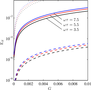
Figure 4: Breathing errors with non-uniform pushing forces. The physical parameters are: $\epsilon=0.04$, $a/d=0.001$, and $\omega\tau=3.5$ (black), $5.5$ (red), and $7.5$ (blue). Results for temperatures of $T=0.125$, 1 and $8\times\hbar\omega/k_{\mathrm{B}}$ are plotted as dashed, full and dotted lines, respectively. For all three temperatures, larger $\tau$ leads to larger $\mathrm{E}_{S}$. $\mathrm{E}_{S}$ is increasing approximately linearly with $G^{2}\tau$, i.e. for fixed $G$, $\mathrm{E}_{S}$ will be proportional to $\tau$, the pulse duration! This is very different from the behavior of $\mathrm{E}_{\mathbf{\overline{q}}}$ above, which is rapidly decreased by increasing $\tau$ and thereby making the push more adiabatic.

We also see that $\mathrm{E}_{S}$ is nearly proportional to $G^{2}\tau$. That larger $G$ leads to larger errors is not surprising, but that larger $\tau$ does is rather counter-intuitive: larger $\tau$ means a more smooth and thus more adiabatic push. It also means a smaller amplitude for the push since the ions will have more time to pick up the gate phase, cf. Eq. (27). Let us discuss the explanation for this behaviour in more detail.

For exponential suppression of errors to be valid, the evolution should be well into the adiabatic regime. At first sight, the relevant timescale is $\omega^{-1}$, the oscillation period of the micro traps. Since the traps are assumed to be far apart ($a\ll d$) the parameter $\epsilon$ is small and the normal modes of the system have periods shifted little from this value: the CM mode is in fact unaffected by the Coulomb interaction and has frequency $\omega$ while the relative motion mode oscillates at $\sqrt{1+\epsilon}\;\omega$. With $\omega\tau\gg 1$ one should therefore not be able to put excitations into either of these modes. However, it is perfectly possible to transfer excitations between the modes, as the adiabatic timescale for this process is $(\sqrt{1+\epsilon}\;\omega-\omega)^{-1}\sim\epsilon^{-1}\omega^{-1}/2$. Such a transfer will be induced by mixing of the CM and relative motion during the gate operation. A linear push potential will not mix the two, but a non-linear one will.

Another effect to remember is that when the instantaneous oscillation frequencies change during the push, the external motion will pick up different phases depending on the number of excitation quanta. Like the transfer of excitations, this effect of course disappears if the system is cooled to the ground state. A perturbative calculation to lowest order in $a/d$, $G$ and $\epsilon$ gives the result

$$E_{S}=\frac{\pi}{20}G^{2}\xi^{2}\omega^{2}\tau^{2}\times\\ \times\Biggl{\{}\frac{1}{\sinh^{2}\left(\hbar\omega/2k_{\mathrm{B}}T\right)}\left[1+\exp\left(-\frac{\epsilon^{2}\omega^{2}\tau^{2}}{8}\right)\right]\\ +2\left[\frac{1}{\sinh^{2}\left(\hbar\omega/2k_{\mathrm{B}}T\right)}+2\right]\exp\left(-2\omega^{2}\tau^{2}\right)\Biggr{\}}.$$ (28)

The prefactor gives the scaling behaviour both in the “naïve” nonadiabatic limit $\omega\tau<1$ and in the more relevant intermediate region $1<\omega\tau<\epsilon^{-1}$:

$$\mathrm{E}_{S}\propto\xi^{2}G^{2}\omega^{2}\tau^{2}\propto\frac{G^{2}\omega\tau}{\epsilon},$$ (29)

In fact, even in the adiabatic limit $\epsilon\omega\tau\gg 1$ this scaling holds true since one term in Eq. (28) does not contain an exponential damping factor with $\tau^{2}$. This unsuppressed term is stemming from the above mentioned effect of time-varying instantaneous mode frequencies.

From Eq. (28) we can also understand the strong temperature dependence of the breathing errors. For $k_{\mathrm{B}}T/\hbar\omega\gg 1$, the breathing errors will scale approximately like $T^{2}$. However, as seen in Figure 4, high temperatures require very low values for $G$. For low temperatures, note that one term in Eq. (28) is not suppressed even at $T=0$. This term stems from changes in the ground state widths of the two instantaneous normal modes and is adiabatically suppressed when $\omega\tau\gg 1$. To find the dominant term for very low temperatures and short pulses one should do a higher order perturbative calculation.

V Optimizing gate performance

From the simulations in Sec. IV we learn that without improvement high fidelities require either very low values of $G$ or cooling the external motion almost to the ground state. In this section we shall see how a better performance can be achieved by modifying the temporal shape of the push-pulses.

V.1 Correcting the phase

Our first step will be to correct the gate phase by a simple scaling of the push pulse-shape. From Fig. 1 we know that typical errors can be well above the percent level. Our strategy is based on the observation that the simplest estimate of the gate-phase suggest that it scales as the square of the push-amplitude, $\xi$. [A general gate-phase replaces the $\pi$ in the numerator of Eq. (27).] We therefore divide $\xi$ by the square-root of the ratio of the observed gate-phase and the ideal gate-phase ($\pi$) and repeat the propagation. In Fig. 5

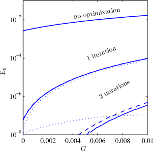
Figure 5: Improving $\mathrm{E}_{\theta}$ by iteratively adjusting the push-amplitude $\xi$. The pulse-duration is $\tau=7.5$ and the other parameters are as in the previous figures. Four sets of curves are shown, each with results for $T=0.125$ (dashed), 1 (full), and 8$\times\hbar\omega/k_{\mathrm{B}}$ (dotted). The uppermost set (looks like a single curve) is for the un-optimized pulse-amplitude and identical to the $\tau=7.5$ curves of Fig. 1. The progressively lower sets are for one and two iterations of the amplitude scaling described in the text. Note that as the error gets smaller, temperature begins to have an effect. This simple adjustment is capable of reducing $\mathrm{E}_{\theta}$ below $10^{-6}$ for all the considered $G<0.01$.

we show the results of applying this algorithm to the $\tau=7.5$ curves of Fig. 1. As can be seen, $\mathrm{E}_{\theta}$ is rapidly reduced and can be brought below e.g. $10^{-6}$ in a very modest number of iterations. For simplicity we ignore the temperature dependent $\text{Tr}[b\gamma]$ contribution to $\mathrm{E}_{\theta}$ when rescaling the pulse. This is the reason for the $k_{\mathrm{B}}T=8\hbar\omega$ (dotted curves) departing from the $k_{\mathrm{B}}T=0.125\hbar\omega$ and $k_{\mathrm{B}}T=1\hbar\omega$ curves especially at low $G$.

V.2 Fast gate: eliminating sloshing in $\mathbf{\overline{x}}$

A big advantage of the simple harmonic approximation is that it becomes feasible to solve the equations of motion many times with different temporal shapes of $f(t)$ in order to optimize the performance of the gate. Rather than simple trial-and-error we will apply the global control algorithm of Krotov, which is guaranteed to improve the performance at each iteration Krotov (1995); Tannor et al. (1992); Sklarz and Tannor (2002). The relevant equations for our case are given in Appendix C.

In general, it is desirable to complete the gate in as short a time as possible. This will limit many undesired effects and it will ultimately enable faster quantum computations. A fast gate, however, means that the pushing force will deliver a rather abrupt impulse. This can lead to excitations of the external motion being left after the completion of the gate, limiting the fidelity. In this section we show how such “sloshing” effects can be avoided by using optimal control.

We start from an initial Gaussian temporal shape of the push. The overall amplitude is first optimized iteratively to get the desired gate phase as described above. We then run the Krotov algorithm to get a better shape of the pulse. We assume a non-uniform pushing force, $G=2\times 10^{-3}$. The result is plotted in Fig. 6.

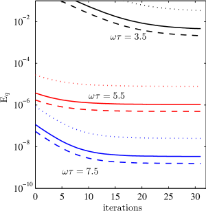
Figure 6: Optimization of pulse-shape to eliminate sloshing. We plot $\mathrm{E}_{\mathbf{\overline{q}}}$, the contribution of sloshing to the total infidelity, as a function of the number of Krotov iterations performed. The parameters in this example are: $\epsilon=0.04$, $a/d=0.001$, $G=2\times 10^{-5}$. Each curve corresponds to a separate value of the pulse duration, $\omega\tau=$3.5, 5.5, 7.5, with larger $\tau$ always giving a lower value of $\mathrm{E}_{\mathbf{\overline{q}}}$.

As can be seen, the influence of sloshing motion can be decreased by a couple of orders of magnitude in a modest number of iterations.

To investigate the physical mechanism behind the reduction of the sloshing error, we plot in the lower panel of Fig. 7

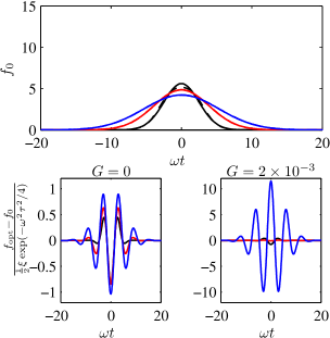
Figure 7: Upper panel: pulse shape both before (full line) and after (dashed line) Krotov optimization. Curves for three different pulse duration are shown, $\omega\tau=3.5$, 5.5 and 7.5, other parameters are as in Fig. 6. Only for the shortest pulse is the optimized curve distinguishable from the original Gaussian. Lower panel: Difference between optimized pulse and initial Gaussian pulse (after adjusting overall amplitude to reduce phase errors). The left plot is for $G=0$, the right plot is for $G=2\times 10^{-3}$. Each curve has been normalized to the prediction of a $G=0$ perturbative calculation, which is seen to describe well the $G=0$ case as all curves have a maximal excursion of approximately -1, while the $G\neq 0$ case is only qualitatively similar.

the difference between the optimized pulse $f_{\mathrm{opt}}(t)$ and the original Gaussian pulse $f_{0}(t)=\xi\exp(-t^{2}/\tau^{2})$. This difference looks a lot like a simple cosine-wave with a period close to $2\pi\omega^{-1}$ multiplied by a Gaussian of the same width as $f_{0}$. Thus the optimized pulse is approximately of the form $f_{\mathrm{opt}}(t)\sim f_{0}(t)+A\cos(\omega t)\exp(-t^{2}/\tau^{2})$. An approximative calculation of the sloshing excitation for the simplest $G=0$ case reveals that for such a pulse, the non-resonant contribution of the bare Gaussian pulse is cancelled by a resonant contribution from the cosine-modulated pulse. Since the resonant response is much stronger, only a small, negative $A$ is needed for this cancellation. More precisely, the optimal $A$ from first order pertubation theory is given by $-\frac{1}{2}\xi\exp(-\omega^{2}\tau^{2}/4)$ and Fig. 7 shows that this is also what the Krotov algorithm converges to for $G=0$. The “strategy” of the Krotov algorithm in this case seems therefore to be well understood. For $G\neq 0$, it is more difficult to predict the value of $A$, but nonetheless the Krotov algorithm seems to be highly efficient.

V.3 Minimizing breathing errors

We now know that phase errors and sloshing errors can be controlled and we turn to the breathing errors of Fig. 4. Without optimization, these errors put rather stringent limits on the parameters. In order to keep $\mathrm{E}_{S}$ at an acceptable level, either very low temperature or very small $G$ is required. For very low temperature $k_{\mathrm{B}}T=0.125\hbar\omega$, we need just $G\lesssim 10^{-2}$ to get $\mathrm{E}_{S}$ below $10^{-4}$, but if we assume a more modest cooling to $k_{\mathrm{B}}T=1\hbar\omega$ the same error-level require $G\lesssim 2\times 10^{-4}$. Note that even at $G=0$, breathing errors persist and that for $k_{\mathrm{B}}T=8\hbar\omega$ they never get below the 10^-5 level. These errors stem from the high order terms in the Coulomb potential which have been ignored in Eq. (28).

As described in Sec. IV.4, breathing errors cannot be eliminated by simply increasing the push duration $\tau$: First of all the adiabatic time-scale is $\sim\epsilon^{-1}\omega^{-1}/2$ which will mean a slow gate and secondly even in that limit errors from the change in normal modes frequencies remain and even increase, cf. discussion below Eq. (29). It turns out that a simple application of the Krotov algorithm is also not very efficient in reducing the breathing errors. A partial explanation for this can be found from the perturbative calculation leading to Eq. (28) and the analysis of sloshing error-reduction above: since the adiabatic time-scale for the breathing errors is long, the Gaussian pulses we consider are not adiabatic w.r.t. breathing errors and thus the admixture of a small resonant component in the push-pulse will not be enough to get the cancellation we found in the case of sloshing errors. In fact, the amplitude of the cosine modulation should be comparable to the total amplitude for the relatively short pulses considered. There is nothing to be gained from a small amplitude modulation and thus the “linear” version of the Krotov algorithm we apply (see Appendix C) will not work.

In fact, in order to cancel out the contribution to the breathing errors due to mode frequency changes, sign changes in the push amplitudes are required during the pulse. This is beyond the simplest physical implementations where the push amplitude is proportional to some laser intensity. In principle it is possible to play with detunings to implement the sign changes, and this will in fact give many of the advantages of the $\pi$-pulse method, see Ref. Šašura and Steane (2003). Allowing negative push amplitudes and putting “by hand” an optimized $\cos(\epsilon\omega t/2)$ modulated contribution, we have been able to e.g. reduce $E_{S}$ below $10^{-6}$ for $\omega\tau=7.5$, $G=2\times 10^{-3}$, and $T=1\times\hbar\omega/k_{\mathrm{B}}$. Compared to the results reported in Fig. 4, this is a reduction by more than 3 orders of magnitude. Unfortunately, the strongly modified pulse now gives rise to large sloshing errors. To obtain an overall safisfactory fidelity we use a combined strategy: we first put the breathing error reduction by hand, then iteratively reduce phase errors and finally use the Krotov algorithm to reduce the sloshing errors. In Fig. 8

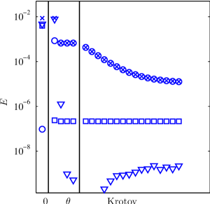
Figure 8: Combined strategy for reducing infidelity for $\epsilon=0.04$ and $G=2\times 10^{-3}$. The three contributions $E_{\theta}$, $E_{q}$, and $E_{S}$ are labeled by $\triangledown$, $\circ$, and $\square$, respectively. Their sum is labeled by $\times$. The leftmost column are the results for a simple Gaussian with $\omega\tau=7.5$. The breathing errors dominate. In the next column, breathing errors have been reduced (but sloshing increased) by using a cosine-modulated pulse based on Eq. (28). The overall amplitude is then iteratively optimized to reduce phase errors as described in Sec. V.1. As can be seen, 3 iterations are more than sufficient to render $E_{\theta}$ completely insignificant. The dominating error type is now sloshing and in the third column, the Krotov algorithm is applied to finally reduced the total infidelity below $10^{-4}$.

we show results of this strategy starting from $\omega\tau=7.5$.

VI Conclusion

In this paper we have shown how a time-dependent, quadratic approximation to the Hamiltonian can be a useful tool when analyzing quantum gates based on conditional external dynamics. The resulting equations are much more manageable than the original two-body Schrödinger equations. This is especially true if one were to include more spatial dimensions than the one considered here: A full time-dependent, three dimensional, two-body wavefunction calculation is an extremely demanding numerical task, whereas the corresponding quadratic approximation will be much more manageable.

We used the developed method to show how to improve on a naïve design of the pushing gate. This was done including a non-uniform contribution to the pushing force. An important lesson of our analysis and simulations, is to pay attention to changes in the symmetry of the Hamiltonian during the gate operation. In the present case, a nonlinear push potential invalidates the separation of the dynamics into CM and relative motion. This opens up another type of non-adiabaticity, namely transfer of excitations between the two normal modes. The adiabaticity parameter for this type of error is $\epsilon\omega\tau$ and for small $\epsilon$, adiabaticity will require gate times much larger than the charateristic time of the micro-traps. An efficient counter-measure is to decrease temperature so that there are in fact no excitations to transfer between modes. Failing that, one should increase $\epsilon$ as much as possible and, somewhat counter-intuitively, do the gate as fast possible. Sloshing errors puts a lower limit on the gate-time, but as we show an optimized choice of the temporal shape of the push can dramatically reduce this problem.

By analyzing the way that the Krotov optimized pulse reduces sloshing errors, we identified the basic mechanism as a destructive interference between the non-resonant, non-adiabatic contribution from the finite push pulse duration and a resonant contribution from a small amplitude superposed oscillation of the push force. Generalizing this idea to deal with breathing errors, we were able to reduce them by several orders of magnitude. However, since breathing errors are not significantly adiabatically suppressed for the considered pulse durations, the destructive interference required sign-changes in the push amplitude, which introduce experimental complications. The suppression of breathing errors also came at the price of increased sloshing errors, but we showed that the Krotov algorithm once again was able to improve the pulse shape.

One may ask to what extent is the final pulse shape optimal for the given overall gate-time? This is an interesting question in general and in this study we saw examples both where the Krotov algorithm seemed to exhaust the potential in its “strategy” (the $G=0$ case in Fig. 7) and where it was not able to find an optimization. In the latter case we could improve the pulse by hand (eliminate the breathing errors by destructive interference). The problem of optimality is related to the question of a quantum speed limit (QSL) Giovannetti et al. (2003) and this connection has been studied in Ref. Caneva et al. (2009). Note, however, that in our case the hamiltonian is time-dependent and what we want is in fact to leave the external motion unaffected after the pulse. It would be interesting to investigate such a general adiabaticity problem along the same lines as the work on the QSL.

Appendix A Evolution under quadratic Hamiltonian

In this section we show that a second order Hamiltonian leads to an evolution operator that can be written like $\hat{U}(t)$ Eq. (12). For alternative parameterizations, see Refs.Gilmore and Yuan (1987, 1989). We will do a direct calculation showing that $\hat{U}(t)$ fulfills the Schrödinger equation

$$i\frac{\partial}{\partial t}\hat{U}=\hat{H}_{\mathrm{so}}\hat{U}.$$ (30)

The demanding part of the the calculation involves differentiating expontials of time dependent operators. A useful formular can be found in e.g. Wilcox (1967) and involves integration over an auxillary variable $\eta$. It results in

$$\begin{split}i\frac{\partial}{\partial t}\hat{D}_{\mathbf{c}}=&\int_{0}^{1}\hat{D}_{\eta\mathbf{c}}\;\dot{\mathbf{c}}^{\mathrm{T}}J\hat{\mathbf{q}}\;\hat{D}_{\eta\mathbf{c}}^{\dagger}\;d\eta\;\hat{D}_{\mathbf{c}}\\ =&\int_{0}^{1}\dot{\mathbf{c}}^{\mathrm{T}}J\left(\hat{\mathbf{q}}-\eta\mathbf{c}\right)\;d\eta\;\hat{D}_{\mathbf{c}}\\ =&\dot{\mathbf{c}}^{\mathrm{T}}J\left(\hat{\mathbf{q}}-\frac{1}{2}\mathbf{c}\right)\hat{D}_{\mathbf{c}}\end{split}$$ (31)

for the displacement operator and

$$\begin{split}i\frac{\partial}{\partial t}\hat{W}_{b}=&\int_{0}^{1}\hat{W}_{\eta b}\;\frac{1}{2}\hat{\mathbf{q}}^{\mathrm{T}}\dot{b}\hat{\mathbf{q}}\hat{W}_{\eta b}^{\dagger}\;d\eta\;\hat{W}_{b}\\ =&\frac{1}{2}\int_{0}^{1}\left(e^{-\eta Jb}\hat{\mathbf{q}}\right)^{\mathrm{T}}\dot{b}\left(e^{-\eta Jb}\hat{\mathbf{q}}\right)\;d\eta\;\hat{W}_{b}\\ =&\frac{1}{2}\hat{\mathbf{q}}^{\mathrm{T}}J^{\mathrm{T}}\int_{0}^{1}e^{\eta Jb}J\dot{b}e^{-\eta Jb}\;d\eta\;\hat{\mathbf{q}}\hat{W}_{b}\\ =&\frac{1}{2}\hat{\mathbf{q}}^{\mathrm{T}}J^{\mathrm{T}}\left(\frac{\partial}{\partial t}e^{Jb}\right)e^{-Jb}\;\hat{\mathbf{q}}\;\hat{W}_{b}\end{split}$$ (32)

for the squeezing operator. It is now easy to show that the equations of motion (14) for $\phi$, $\mathbf{c}$ and $S=\exp(Jb)$ leads to $\hat{U}=\exp(-i\phi)\hat{D}_{\mathbf{c}}\hat{W}_{b}$ fulfilling Eq. (30) .

Appendix B Fidelity for Gaussian evolutions

In this section we derive expressions for the fidelity as a function of the variables used to characterize the evolution in the harmonic approximation, $\phi_{\beta}$, $\mathbf{\overline{q}}_{\beta}$, and $S_{\beta}$, $\beta=00,01,10,11$.

If we assume that the initial state of the system is a product of an internal state density matrix and an external state density matrix, $\rho\otimes\sigma$, we get the following state for the internal degrees of freedom after the application of $\hat{U}^{\text{tot}}$ of Eq. (2):

$$\begin{split}\rho^{\prime}=&\text{Tr}_{\text{ex}}\left[\hat{U}^{\text{tot}}\rho\otimes\sigma\left(\hat{U}^{\text{tot}}\right)^{\dagger}\right]\\ =&\sum_{\alpha\beta}|\alpha\rangle\!\langle\beta|\;[\rho\circ R]_{\alpha\beta}.\end{split}$$ (33)

Here “$\circ$” denotes the element-wise matrix product (the Hadamard product) and $R$ is the matrix given by:

$$[R]_{\alpha\beta}=\text{Tr}\left[\hat{U}^{\text{ex}}_{\alpha}\sigma\left(\hat{U}^{\text{ex}}_{\beta}\right)^{\dagger}\right]$$ (34)

It is easy to see that $R$ er Hermitian and that all its diagonal elements are 1. In particular, $\text{Tr}R=4$. Slightly less obvious is it that $R$ is positive semi-definite: Let $c\in\mathbb{C}^{4}$. Then:

$$\begin{split}c^{\dagger}Rc&=\text{Tr}\left[\bigl{\{}\sum c_{\alpha}^{*}\hat{U}^{\text{ex}}_{\alpha}\bigr{\}}\sigma\bigl{\{}\sum c_{\beta}\left(\hat{U}^{\text{ex}}_{\beta}\right)^{\dagger}\bigr{\}}\right]\\ &=\text{Tr}\left[\bigl{\{}\sum c_{\beta}^{*}\hat{U}^{\text{ex}}_{\beta}\bigr{\}}^{\dagger}\bigl{\{}\sum c_{\alpha}^{*}\hat{U}^{\text{ex}}_{\alpha}\bigr{\}}\sigma\right]\geq 0\end{split}$$ (35)

where we have used the cyclic property of the trace and the fact that the trace of a product of positive semi-definite operators is non-negative.

The element-wise product form in Eq. (33) is perhaps not the most illuminating. If we diagonalize $R=\sum_{h}w_{h}w_{h}^{\dagger}$, we get instead a Krauss operator sum form:

$$\rho^{\prime}=\sum_{h=1}^{4}K_{h}\rho K_{h}^{\dagger}$$ (36)

with $K_{h}=\mathrm{diag}(w_{h})$.

There are different ways to define the fidelity of the gate. The one used in Refs. Šašura and Steane (2003) and Calarco et al. (2001) is as the minimum fidelity of the obtained final state w.r.t. the wanted final state when the input state is varied. This means that

$$F_{\min}=\min_{\psi}\langle\psi|U_{0}^{\dagger}\rho_{\psi}^{\prime}U_{0}|\psi\rangle$$ (37)

with $\rho_{\psi}=|\psi\rangle\!\langle\psi|$ and $U_{0}$ the gate operator we aim for. In the case of a phase gate, $U_{0}$ is diagonal in the logical state basis:

$$\hat{U}_{0}=\sum_{\beta}|\beta\rangle\!\langle\beta|e^{i\theta_{\beta}}$$ (38)

and we get the simpler minimization problem:

$$F_{\min}=\min_{\{p_{i}\}}p^{\mathrm{T}}\tilde{R}p$$ (39)

where the $p\in\mathbb{R}_{+}^{4}$ and $\sum p_{i}=1$. The matrix $\tilde{R}=U_{0}RU_{0}^{\dagger}$ is Hermitian, but since $p$ is confined to be real, only its real symmetric part contributes. The minimization in Eq. (39) is a so-called quadratic programming problem and very efficient numerical methods for its solution exist. Given $\tilde{R}$ it is therefore simple to calculate $F_{\min}$ on the computer. However, a more direct evaluation is possible if fidelity is instead defined as an average over input states as

$$F_{\mathrm{avg}}=\int_{S^{2n-1}}\langle\psi|U_{0}^{\dagger}\rho_{\psi}^{\prime}U_{0}|\psi\rangle\;dV.$$ (40)

Here $S^{2n-1}$ denotes the normalized states (unit sphere) in $\mathbb{C}^{n}$ and the volume element $dV$ is such that $\int_{S^{2n-1}}dV=1$. For $F_{\mathrm{avg}}$ a compact formula exist Pedersen et al. (2007) and using it in the present case leads to

$$F_{\mathrm{avg}}=\frac{1}{4(4+1)}\left(\text{Tr}\tilde{R}+\sum_{\alpha\beta}\tilde{R}_{\alpha\beta}\right)$$ (41)

or when using the properties of $\tilde{R}$:

$$1-F_{\mathrm{avg}}=\frac{1}{10}\sum_{\alpha<\beta}\left(1-\mathrm{Re}\left[\tilde{R}_{\alpha\beta}\right]\right).$$ (42)

B.1 General small errors

Typically, we will be mostly interested in situations where the four logical states leads to almost identical evolutions for the external states. It is then useful to write

$$\begin{split}\hat{U}^{\text{ex}}_{\beta}=&\exp(i\hat{D}_{\beta})\hat{U}^{\text{ex}}_{\mathrm{com}}\\ =&\exp\left(i\langle\hat{D}_{\beta}\rangle\right)\exp(i\Delta\hat{D}_{\beta})\hat{U}^{\text{ex}}_{\mathrm{com}},\end{split}$$ (43)

where $\langle\hat{D}\rangle=\text{Tr}\left[\hat{D}\hat{U}^{\text{ex}}_{\mathrm{com}}\sigma_{\mathrm{ex}}(\hat{U}_{\mathrm{com}}^{\text{ex}})^{\dagger}\right]$ and $\Delta\hat{D}=\hat{D}-\langle\hat{D}\rangle$. Calculating $\tilde{R}$ to second order in the $\Delta\hat{D}$’s, we get:

$$\begin{split}\tilde{R}_{\alpha\beta}=&\exp\left(i\Delta\theta_{\alpha}\right)\\ &\times\left\{1-\frac{1}{2}\left\langle\Delta\hat{D}_{\alpha}^{2}+\Delta\hat{D}_{\beta}^{2}-2\Delta\hat{D}_{\alpha}\Delta\hat{D}_{\beta}\right\rangle\right\}\\ &\phantom{=}\times\exp\left(-i\Delta\theta_{\beta}\right).\end{split}$$ (44)

This form is useful, as it separates the infidelity into systematic phase-errors (the $\exp(\pm i\Delta\theta_{\alpha})$ factors) and “decoherence” (factor in curly brackets). The phase errors $\Delta\theta_{\beta}=\langle\hat{D}_{\beta}\rangle-\theta_{\beta}$ can be made small by tuning the average of laser powers etc. and this can usually be done very well. The challenge will therefore most often be to suppress the fluctuations, i.e., the terms in curly brackets in Eq. (44).

Assuming also the $\Delta\theta$’s to be small, Eq. (42) becomes:

$$1-F_{\mathrm{avg}}=\frac{1}{20}\sum_{\alpha<\beta}\left(\left[\Delta\theta_{\alpha}-\Delta\theta_{\beta}\right]^{2}+\left\langle\left(\Delta\hat{D}_{\alpha}-\Delta\hat{D}_{\beta}\right)^{2}\right\rangle\right).$$ (45)

At first sight, this form might seem dubious since only differences in the $\Delta\theta$’s and $\Delta\hat{D}$’s enter. However, one should remember that any common evolution on the four branches can be absorbed into $\hat{U}^{\text{ex}}_{\mathrm{com}}$ in Eq. (43). This emphasizes that for the implementation of a single gate on the logical state, the external motion must not necessarily be returned to its initial state as long as the final state is common to all logical input states. Typically, the further requirement that energy is not pumped into the external degrees of freedom by repeated application of the gate must be made. In the particular case of the pushing gate, this requirement is in fact already hidden in Eq. (45) since the $\beta=00$ branch contains no pushing. In other cases, one could apply cooling to the external state between gate operations.

B.2 The non-local part of the phase

We are seeking to implement the phase-gate (38). In many cases, the $\theta_{\beta}$’s are not so important individually since single-particle operations are easy to perform and only the truely non-local phase is interesting. Assuming that perfect single-particle phase changes can be implemented on average, it is straightforward to show that one should replace $\sum_{\alpha<\beta}[\Delta\theta_{\alpha}-\Delta\theta_{\beta}]^{2}$ by

$$\left[\Delta\theta_{00}-\Delta\theta_{01}-\Delta\theta_{10}+\Delta\theta_{11}\right]^{2}$$ (46)

in Eq. (45).

This simplified view of single-particle phase-changes should of course be revisited in a more complete analysis of any given proposal for quantum-computing. In the present work we use the replacement (46) throughout, but let us emphasize that fluctuations in the single-particle phaserotations are more naturally incorporated in the $\Delta\hat{D}$ terms of Eq. (45) than in the $\Delta\theta$ terms: One simply model the fluctations as a consequence of some fluctuating parameter which can be included in $\sigma_{\mathrm{ex}}$.

B.3 The Gaussian case

For Gaussian evolutions like (12) and a Gaussian (e.g. thermal) external state $\sigma$ with covariance matrix

$$\begin{split}\gamma_{ij}=&\frac{1}{2}\langle q_{i}q_{j}+q_{j}q_{i}\rangle-\langle q_{i}\rangle\langle q_{j}\rangle\\ =&\mathrm{Re}\text{Tr}\left[q_{i}q_{j}\sigma\right]-\text{Tr}\left[q_{i}\sigma\right]\text{Tr}\left[q_{j}\sigma\right]\end{split}$$ (47)

and vanishing means

$$\langle q_{i}\rangle=\text{Tr}\left[q_{i}\sigma\right]=0$$ (48)

one gets phase contributions

$$\langle\hat{D}_{\beta}\rangle=-\phi_{\beta}-\text{Tr}\left[b_{\beta}\gamma\right]$$ (49)

and decoherence terms

$$\left\langle\left(\Delta D_{\alpha}-\Delta D_{\beta}\right)^{2}\right\rangle=(c_{\alpha}-c_{\beta})^{\mathrm{T}}J\gamma J^{\mathrm{T}}(c_{\alpha}-c_{\beta})\\ +\frac{1}{2}\text{Tr}\left[(b_{\alpha}-b_{\beta})\gamma(b_{\alpha}-b_{\beta})\gamma\right]\\ +\frac{1}{8}\text{Tr}\left[(b_{\alpha}-b_{\beta})J(b_{\alpha}-b_{\beta})J\right]$$ (50)

In general, for a harmonic oscillator in thermal equilibrium at temperature $T$, the covariance matrix is given by

$$\gamma_{\mathrm{thermal}}=\frac{1}{2}\frac{1}{\tanh\frac{\hbar\omega}{2k_{B}T}}\begin{bmatrix}\frac{\hbar}{m\omega}&0\\ 0&\hbar m\omega\end{bmatrix}$$ (51)

where $k_{B}$ is the Boltzmann constant. In the present case, the CM and the relative motion are separately in thermal equilibrium and for the corresponding dimensionless position and momentum operators [$x_{\mathrm{CM}}=(x_{1}+x_{2})/2$ etc.], we get:

$$\gamma=\gamma_{\mathrm{CM}}\oplus\gamma_{\mathrm{rel}}$$ (52)

with

$$\gamma_{\mathrm{rel}}=\frac{1}{2}\frac{1}{\tanh\frac{(1+\epsilon)^{1/2}\hbar\omega}{2k_{B}T}}\begin{bmatrix}\frac{2}{(1+\epsilon)^{1/2}}&0\\ 0&\frac{(1+\epsilon)^{1/2}}{2}\end{bmatrix}$$ (53)

and

$$\gamma_{\mathrm{CM}}=\frac{1}{2}\frac{1}{\tanh\frac{\hbar\omega}{2k_{B}T}}\begin{bmatrix}\frac{1}{2}&0\\ 0&2\end{bmatrix}.$$ (54)

In the limit $\epsilon\ll 1$, a we have approximately $\gamma\propto\mathbb{I}_{4}$ if we use the set of individual-ion operators $(x_{1},x_{2},p_{1},p_{2})$.

Appendix C The Krotov Algorithm

Optimizing the temporal shape of the push pulse is done using the Krotov algorithm Krotov (1995). For an introduction to the method, see e.g. Ref. Sklarz and Tannor (2002).

C.1 Auxillary variables

The key ingredient in this approach is a function $\Phi(t,\{\phi_{\beta},\mathbf{\overline{q}}_{\beta},S_{\beta}\}_{\beta=00,01,10,11})$ which allow us to translate the global goal of improving the final $\hat{U}^{\text{tot}}(T)$ to a local problem of choosing a better $f(t)$ for each $t$. Constructing $\Phi$ is in general very difficult, but it is relatively simple to get a linear approximation to it. The coefficients in this approximation will constitute a set of auxillary variables. For each branch, the equations of motion for the auxillary variables $\tilde{\phi}_{\beta}$, $\mathbf{\tilde{q}}_{\beta}$ and $\tilde{S}_{\beta}$ are determined by the requirement that they are conjugate to the physical variables $\phi_{\beta}$, $\mathbf{\overline{q}}_{\beta}$, and $S_{\beta}$, respectively.

Let us focus on a single branch and suppres the $\beta$ index like in Sec. II.1. We then need to construct $\mathcal{H}(t;\phi,\mathbf{\overline{q}},S;\tilde{\phi},\mathbf{\tilde{q}},\tilde{S})$ such that Eqs. (14) can be written

$$\frac{\partial}{\partial t}\phi =\frac{\partial}{\partial\tilde{\phi}}\mathcal{H}$$ (55)

$$\frac{\partial}{\partial t}\overline{q}_{i} =\frac{\partial}{\partial\tilde{q}_{i}}\mathcal{H}$$ (56)

$$\frac{\partial}{\partial t}S_{ij} =\frac{\partial}{\partial\tilde{S}_{ij}}\mathcal{H}.$$ (57)

This leads simply to

$$\begin{split}\mathcal{H}(t;\phi,\mathbf{\overline{q}},S;\tilde{\phi},\mathbf{\tilde{q}},\tilde{S})&=\tilde{\phi}\Bigl{[}E(t,\mathbf{\overline{x}})-\frac{1}{2}\mathbf{F}^{\mathrm{T}}(t,\mathbf{\overline{x}})\Bigr{]}\\ &\phantom{=}+\mathbf{\tilde{q}}^{\mathrm{T}}\Bigl{[}Jh(t,\mathbf{\overline{x}})\mathbf{\overline{q}}-J\mathbf{F}(t,\mathbf{\overline{x}})\Bigr{]}\\ &\phantom{=}+\text{Tr}\Bigl{[}\tilde{S}^{\mathrm{T}}Jh(t,\mathbf{\overline{x}})S\Bigr{]}\end{split}$$ (58)

Then the equations of motion for the auxillary variables become

$$\frac{\partial}{\partial t}\tilde{\phi} =-\frac{\partial}{\partial\phi}\mathcal{H}=0$$ (59)

$$\frac{\partial}{\partial t}\mathbf{\tilde{q}} =-\nabla_{\mathbf{\overline{q}}}\mathcal{H}$$ (60)

$$\frac{\partial}{\partial t}\tilde{S} =\nabla_{S}\mathcal{H}=h(t,\mathbf{\overline{x}})J\tilde{S}.$$ (61)

The equation of motion for $\mathbf{\tilde{q}}$ is rather involved since $\mathcal{H}$ depends on $\mathbf{\overline{x}}$ in a complicated manner through $h$, $F$ and $E$. It can be rewritten as two coupled time-dependent, forced harmonic oscillators. Note on the other hand that $\tilde{\phi}$ is time-independent and that $J\tilde{S}$ solves the same equation as $S$.

C.2 Objective function

Our ultimate goal is to improve the fidelity of the gate. However, it is somewhat impractical to apply this as the objective in the Krotov algorithm: Calculating the fidelity is only simple for small errors and in general it depends on e.g. the temperature of the external motion. Instead we shall work with a simpler function of the variables $\phi$, $\mathbf{\overline{q}}$ and $S$ for the four branches. The reduction of this objective function should tend to increase the fidelity of the gate. Based on the fact that in the pushing gate, the branch $\beta=00$ is not subject to any time-dependent forces, we choose the following:

$$\begin{split}\mathcal{J}&\left(\{\phi_{\beta},\mathbf{\overline{q}}_{\beta},S_{\beta}\}_{\beta=00,01,10,11}\right)=\mathcal{J}_{\phi}+\mathcal{J}_{q}+\mathcal{J}_{S}\\ &\phantom{\beta}=\frac{1}{2}\Bigl{[}\phi_{00}-\phi_{01}-\phi_{10}+\phi_{11}-\pi\Bigr{]}^{2}\\ &\phantom{\beta=}+\frac{1}{2}\sum_{\beta}\left[\Bigl{(}\mathbf{x}_{\beta}-\mathbf{x}_{00}\Bigr{)}^{2}+\Bigl{(}\mathbf{p}_{\beta}-\mathbf{p}_{00}\Bigr{)}^{2}\right]\\ &\phantom{\beta=}+\frac{1}{2}\sum_{\beta}\text{Tr}\left[\Bigl{(}S_{\beta}-S_{00}\Bigr{)}^{\mathrm{T}}\Bigl{(}S_{\beta}-S_{00}\Bigr{)}\right].\end{split}$$ (62)

The term with $\phi$’s aim to ensure the correct phase in the phasegate, while the other terms aim at identical evolution for the external motin in the four branches. In the limit $\epsilon\ll 1$ Eq. (45) formally justifies the use of our chosen objective function, given the extra proviso that we are only interested in the non-local part of the phase.

C.3 Terminal conditions

The objective function supplements the auxillary-variable equations of motion (59–61) with the following terminal conditions, i.e. boundary conditions at $t=T$:

$$\tilde{\phi}_{\beta} (T)=\left.-\frac{\partial}{\partial\phi_{\beta}}\mathcal{J}\right|_{T}$$

$$=-(-1)^{\beta}\left.\bigl{(}\phi_{00}-\phi_{01}-\phi_{10}+\phi_{11}-\pi\bigr{)}\right|_{T}$$ (63)

$$\mathbf{\tilde{x}}_{\beta} (T)=\left.-\nabla_{\mathbf{\overline{x}}_{\beta}}\mathcal{J}\right|_{T}$$

$$=\begin{cases}\left.-\Bigl{(}3\mathbf{\overline{x}}_{00}-\mathbf{\overline{x}}_{01}-\mathbf{\overline{x}}_{10}-\mathbf{\overline{x}}_{11}\Bigr{)}\right|_{T},&\beta=00\\ \left.-\Bigl{(}\mathbf{\overline{x}}_{\beta}-\mathbf{\overline{x}}_{00}\Bigr{)}\right|_{T},&\beta\neq 00\end{cases}$$ (64)

$$\mathbf{\tilde{p}}_{\beta} (T)=\left.-\nabla_{\mathbf{\overline{p}}_{\beta}}\mathcal{J}\right|_{T}$$

$$=\begin{cases}\left.-\Bigl{(}3\mathbf{\overline{p}}_{00}-\mathbf{\overline{p}}_{01}-\mathbf{\overline{p}}_{10}-\mathbf{\overline{p}}_{11}\Bigr{)}\right|_{T},&\beta=00\\ \left.-\Bigl{(}\mathbf{\overline{p}}_{\beta}-\mathbf{\overline{p}}_{00}\Bigr{)}\right|_{T},&\beta\neq 00\end{cases}$$ (65)

$$\tilde{S}_{\beta} (T)=\left.-\nabla_{S_{\beta}}\mathcal{J}\right|_{T}$$

$$=\begin{cases}\left.-\Bigl{(}3S_{00}-S_{01}-S_{10}-S_{11}\Bigr{)}\right|_{T},&\beta=00\\ \left.-\Bigl{(}S_{\beta}-S_{00}\Bigr{)}\right|_{T},&\beta\neq 00\end{cases}$$ (66)

where $(-1)^{\beta}$ is $+1$ for $\beta=00$ and $11$ and $-1$ for $\beta=01$ and $10$. These equations express the values of the auxillary varibles at time $t=T$ in terms of the physical varibles also at $t=T$ and give the input to the backwards propagation of the auxillary variables, cf. Ref. Krotov (1995).

References

- Cirac and Zoller (1995) J. I. Cirac and P. Zoller, Phys. Rev. Lett. 74, 4091 (1995).
- Cirac and Zoller (2000) J. I. Cirac and P. Zoller, Nature 404, 579 (2000).
- Jaksch et al. (1999) D. Jaksch, H.-J. Briegel, J. I. Cirac, C. W. Gardiner, and P. Zoller, Phys. Rev. Lett. 82, 1975 (1999).
- Calarco et al. (2000) T. Calarco, E. A. Hinds, D. Jaksch, J. Schmiedmayer, J. I. Cirac, and P. Zoller, Phys. Rev. A 61, 022304 (2000).
- Burkard et al. (1999) G. Burkard, D. Loss, and D. P. DiVincenzo, Phys. Rev. B 59, 2070 (1999).
- DiVincenzo (2000) D. P. DiVincenzo, Fortschr. Phys. 48, 771 (2000).
- D’Alessandro (2008) D. D’Alessandro, Introduction to quantum control and dynamics, Chapman & Hall/CRC applied mathematics and nonlinear science series (CRC Press, Boca Raton, FL, 2008).
- Calarco et al. (2001) T. Calarco, J. I. Cirac, and P. Zoller, Phys. Rev. A 63, 062304 (2001).
- Šašura and Steane (2003) M. Šašura and A. M. Steane, Phys. Rev. A 67, 062318 (2003).
- Häffner et al. (2003) H. Häffner, S. Gulde, M. Riebe, G. Lancaster, C. Becher, J. Eschner, F. Schmidt-Kaler, and R. Blatt, Phys. Rev. Lett. 90, 143602 (2003).
- Kaplan et al. (2002) A. Kaplan, M.F. Andersen, and N. Davidson, Phys. Rev. A 66, 045401 (2002).
- Krotov (1995) V. F. Krotov, Global methods in optimal control theory, no. 195 in Monographs in pure and applied mathematics (Marcel Dekker, Inc., New York, 1995).
- Sklarz and Tannor (2002) S. E. Sklarz and D. J. Tannor, Phys. Rev. A 66, 053619 (2002).
- Tannor et al. (1992) D. Tannor, V. Kazakov, and V. Orlov, in Time Dependent Quantum Molecular Dynamics, edited by J. Broeckhove and L. Lathouwers (Plenum Press, New York, 1992), vol. 299 of NATO ASI Ser. B, p. 347.
- Giovannetti et al. (2003) V. Giovannetti, S. Lloyd, and L. Maccone, Phys. Rev. A 67, 052109 (2003).
- Caneva et al. (2009) T. Caneva, M. Murphy, T. Calarco, R. Fazio, S. Montangero, V. Giovannetti, and G. E. Santoro (2009), eprint arXiv:0902.4193v1.
- Gilmore and Yuan (1987) R. Gilmore and J.-M. Yuan, J. Chem. Phys. 86, 130 (1987), URL http://link.aip.org/link/?JCP/86/130/1.
- Gilmore and Yuan (1989) R. Gilmore and J.-M. Yuan, J. Chem. Phys. 91, 917 (1989), URL http://link.aip.org/link/?JCP/91/917/1.
- Wilcox (1967) R. M. Wilcox, J. Math. Phys. 8, 962 (1967).
- Pedersen et al. (2007) L. H. Pedersen, N. M. Møller, and K. Mølmer, Phys. Lett. A 270, 47 (2007), eprint quant-ph/0701138.
- Littlejohn (1986) R. G. Littlejohn, Phys. Rep. 138, 193 (1986).