High precision orbital and physical parameters of double-lined spectroscopic binary stars - HD78418, HD123999, HD160922, HD200077 and HD210027

Abstract

We present high precision radial velocities (RVs) of double-lined spectroscopic binary stars HD78418, HD123999, HD160922, HD200077 and HD210027. They were obtained based on the high resolution echelle spectra collected with the Keck I/Hires, Shane/CAT/Hamspec and TNG/Sarge telescopes/spectrographs over the years 2003-2008 as a part of TATOOINE search for circumbinary planets. The RVs were computed using our novel iodine cell technique for double-line binary stars which relies on tomographically disentangled spectra of the components of the binaries. The precision of the RVs is of the order of 1-10 m s^-1 and to properly model such measurements one needs to account for the light time effect within the binary’s orbit, the relativistic effects and the RV variations due to the tidal distortions of the components of the binaries. With such proper modeling, our RVs combined with the archival visibility measurements from the Palomar Testbed Interferometer allow us to derive very precise spectroscopic/astrometric orbital and physical parameters of the binaries. In particular, we derive the masses, the absolute K and H band magnitudes and the parallaxes. The masses together with the absolute magnitudes in the K and H bands enable us to estimate the ages of the binaries.

These RVs allow us to obtain some of the most accurate mass determinations of binary stars. The fractional accuracy in $m\sin i$ only and hence based on the RVs alone ranges from 0.02% to 0.42%. When combined with the PTI astrometry, the fractional accuracy in the masses ranges in the three best cases from 0.06% to 0.5%. Among them, the masses of HD210027 components rival in precision the mass determination of the components of the relativistic double pulsar system PSR J0737-3039. In the near future, for double-lined eclipsing binary stars we expect to derive masses with a fractional accuracy of the order of up to $\sim$0.001% with our technique. This level of precision is an order of magnitude higher than of the most accurate mass determination for a body outside the Solar System — the double neutron star system PSR B1913+16.

1. Introduction

The first observations of a spectroscopic binary star, $\zeta$ UMa (Mizar), were announced by Edward C. Pickering (1846-1919) on 13 November 1889 during a meeting of the National Academy of Sciences in Philadelphia (Pickering, 1890). A similar announcement about $\beta$ Per (Algol) was made by Herman C. Vogel (1841-1907) on 28 November 1889 during a session of Konglich-Preussiche Akademie der Wissenschaften (Vogel, 1890a, b). Even though a transatlantic telegraph cable had been available since the 1860s, it was quite unusual timing for a pre-astro-ph era. Pickering noted that the K line of Mizar occasionally appeared double and this way discovered the first double-lined spectroscopic binary star. Vogel measured radial velocities (RVs) of Algol and used them to prove that the known variations in the brightness of Algol are indeed caused by a “dark satellite revolving about it” (Vogel, 1890b).

Vogel and collaborators built a series of prism spectrographs for the 30-cm refractor of the Potsdam Astrophysical Observatory (Vogel, 1900). In 1888, they initiated a photographic radial-velocity program. Vogel was not the first to take a photograph of a stellar spectrum but improved the technique and obtained an RV precision of 2-4 km s^-1 (Vogel, 1891). Vogel (1906) and Pickering (1908) were both awarded the Bruce medal. Yet another Bruce medalist (1915), William W. Campbell (1862-1938) and collaborators carried out a large spectroscopic program at the Lick Observatory and discovered many spectroscopic binaries (Campbell et al., 1911). They prepared the first catalog of spectroscopic binaries (Campbell & Curtis, 1905). Vogel was the director of the Potsdam Observatory for 25 years, Pickering of the Harvard College Observatory for 42 years and Campbell of the Lick Observatory for 30 years. The administrative duties must have been not too distracting those days.

Both Vogel and Campbell recognized the importance of flexure and temperature control of a spectrograph (Vogel, 1890c; Campbell, 1898, 1900) and Campbell also noted the issue of a slit illumination and its impact on RV precision (Campbell, 1916). Today a high RV precision is achieved by either using a very stable fiber fed spectrograph that is contained in a controlled environment (a vacuum tank) or using an absorption cell to superimpose a reference spectrum onto a stellar spectrum and this way measure and account for the systematic RV errors. Current state of the art precision is at the level of $\sim$1 m s^-1. It is however important to note that such a precision refers to single stars or at best single-lined spectroscopic binaries where the influence of the secondary spectrum can be neglected. In such a case, given a stable spectrograph, an RV measurement is essentially a measurement of a shift of an otherwise constant shape (spectrum).

Radial velocities (RVs) of double-lined spectroscopic binary stars (SB2) can be used effectively to derive basic parameters of stars if the stars happen to be eclipsing or their astrometric relative orbit can be determined. It is quite surprising that the RV precision of double-lined binary stars on the average has not improved much over the last 100 years (see Fig. 1). With the exception of our previous work (Konacki, 2005, 2009a), the RV precision for such targets typically varies from $\sim$0.1 km s^-1 to $\sim$1 km s^-1 and clearly is much worse than what has been achieved for stars with planets or single-lined binary stars. The main problem with double-lined binary stars is that one has to deal with two sets of superimposed spectral lines whose corresponding radial velocities change considerably with typical amplitudes of $\sim$ 50-100 km s^-1. In consequence a spectrum is highly variable and obviously one cannot measure RVs by noting a simple shift.

We have developed a novel iodine cell based approach that employs a tomographic disentangling of the component spectra of SB2s and allows one to measure RVs of the components of SB2s with a precision of the order 1-10 m s^-1 (Konacki, 2009a; Konacki et al., 2009b). Such quality RVs not only enable us to search for circumbinary extrasolar planets (Konacki et al., 2009b) but also to determine basic parameters of stars with an unprecedented precision. In particular the masses of stars for non eclipsing SB2s can be easily determined with a fractional accuracy of the order of at least $\sim$$0.1\%$ and often even $\sim$$0.01\%$. Moreover, we expect that the accuracy in masses will reach $\sim$$0.001\%$ level when our method is applied to eclipsing binary stars. Such a level of precision is an order of magnitude higher than of the most accurate mass determination for a body outside the Solar System — the double neutron star system PSR B1913+16 (Nice et al., 2008).

Below we present our precision RV data sets for five targets HD78418, HD123999, HD160922, HD200077 and HD210027 from our on-going TATOOINE (The Attempt To Observe Outer-planets In Non-single-stellar Environments) RV program to search for circumbinary planets. All of them have been extensively observed with the Palomar Testbed Interferometer (Colavita et al., 1999a, PTI;). The archival PTI visibility measurements can be used to derive relative astrometric orbits of the binaries. These combined with our spectroscopic orbits allow for a complete orbital and physical description of the systems (with the exception of the radii of the components). In §2 we describe the RV measurements and their modeling and in §3 the visibility measurements and their modeling. In §4 we present the spectroscopic and astrometric orbital solutions and the resulting orbital and physical parameters of the binaries. A discussion is provided in §5.

2. Radial velocities

2.1. Iodine absorption cell and spectroscopic binary stars

In the iodine cell (I₂) technique, the Doppler shift of a star spectrum $\Delta\lambda$ is determined by solving the following equation (Marcy & Butler, 1992).

$$I(\lambda)=[F(\lambda+\Delta\lambda_{s})\,T(\lambda+\Delta\lambda_{I_{2}})]\,\otimes\,PSF$$ (1)

where $\Delta\lambda_{s}$ is the shift of the star spectrum, $\Delta\lambda_{I_{2}}$ is the shift of the iodine transmission function $T$, $\otimes$ represents a convolution and $PSF$ a spectrograph’s point spread function (PSF). The parameters $\Delta\lambda_{s},\Delta\lambda_{I_{2}}$ as well as parameters describing the PSF are determined by performing a least-squares fit to the observed (through the iodine cell) spectrum $I$. For this purpose, one also needs (1) a high SNR star spectrum taken without the cell, $F$ (the intrinsic stellar spectrum), which serves as a template for all the spectra observed through the cell and (2) the I₂ transmission function $T$ obtained with a Fourier Transform Spectrometer such as the one at the Kitt Peak National Observatory. The Doppler shift of a star spectrum is then given by $\Delta\lambda=\Delta\lambda_{s}-\Delta\lambda_{I_{2}}$. Such an iodine technique can only be applied to single stars. This is dictated by the need to supply an observed template spectrum of a star in Eq. 1. In the case of SB2s, it cannot be accomplished since their spectra are always composite and time variable.

We can measure precise radial velocities of both components of an SB2 with an I₂ absorption cell by performing the following steps. First, contrary to the standard approach for single stars, we always take two subsequent exposures of a binary target — one with and the other without the I₂ cell. This way we obtain an instantaneous template which is used to model only the adjacent exposure taken with the cell. Next, we perform the usual least-squares fit and obtain the parameters described in Eq. 1. Obviously, the derived Doppler shift, $\Delta\lambda_{i}$ (where $i$ denotes the epoch of the observation), carries no meaning since each time a different template is used (besides it describes a Doppler “shift” of a composite spectrum different at each epoch). However, the parameters (in particular the wavelength solution and the parameters describing PSF) are accurately determined and can be used to extract the star spectrum, $I^{\star,t}(\lambda)$, for each epoch $t$, by inverting the equation 1

$$I^{\star,t}(\lambda)=[I^{t}(\lambda)\,\otimes^{-1}\,PSF^{t}]/T(\lambda)$$ (2)

where $\otimes^{-1}$ denotes deconvolution and $PSF^{t}$, symbolically, the set of parameters describing PSF at the epoch $t$. Such a star spectrum has an accurate wavelength solution, is free of the I₂ lines and the influence of a varying PSF. In the final step, the velocities of both components of a binary target can be measured with the well known two-dimensional cross-correlation technique TODCOR (Zucker & Mazeh, 1994) using as templates the synthetic spectra derived with the ATLAS 9 and ATLAS 12 programs (Kurucz, 1995) and matched to the observed template spectrum, $F(\lambda)$.

2.2. Iodine cell data pipeline

In our data pipeline the reduction process involves the following procedures. An observed stellar spectrum, $I$, is a convolution of an intrinsic stellar spectrum, $F$, with a spectrographs’ PSF, $\psi$. Such a convolution in a discrete form can be written as (Valenti et al., 1995; Endl et al., 2000)

$$I_{i}=\sum_{j=i-r}^{i+r}F_{j}\psi_{i-j},\quad i=1,\dots,N$$ (3)

where $N$ is the number of pixels in the analyzed spectrum and $r$ is the range of PSF such as $\psi_{l}=0$ for $|l|>r$. It is beneficial to work with an oversampled version of the above equation

$$I_{i}=\sum_{j=oi}^{o(i+1)-1}\left(\sum_{k=j-r}^{j+r}F_{k}\psi_{j-k}\right),\quad i=1,\dots,N$$ (4)

where $o$ is the oversampling factor. This equation can be rewritten into two other useful formulas

$$I_{i}=\sum_{j=-r}^{r}\left(\sum_{k=0}^{o-1}F_{j+k+oi}\right)\psi_{-j},\quad i=1,\dots,N$$ (5)

and

$$I_{i}=\sum_{j=-r}^{r+o-1}\left(\sum_{k=-j}^{o-j-1}\psi_{k}\right)F_{j+oi},\quad i=1,\dots,N$$ (6)

They constitute a set of equations which can be written in the form ${\bf I}={\mathbb{R}}{\bf X}$ where ${\bf I}$ represents a vector of the observed spectrum $I_{i},i=1,\dots,N$ and ${\bf X}$ represents a vector of the PSF $\psi_{l},l=-r,\dots,r$ or of the intrinsic stellar spectrum $F_{k},k=1,...,oN+2r$. The matrix ${\mathbb{R}}$ can be easily inferred from the appropriate sums above. By solving the equation 5 one can derive the PSF given the observed and intrinsic stellar spectrum and by solving the equation 6 one can derive the intrinsic stellar spectrum given the PSF and the observed spectrum. The latter process is obviously a deconvolution. The remaining needed set of equations is one that allows us to clean a stellar spectrum observed through an iodine cell from the iodine lines as it is symbolically described in the equation 2. This can be easily achieved by noting that in such a case $F_{k}$ in the equation 6 has to be replaced by $F_{k}T_{k}$ where $T_{k}$ is a known transmission function of the iodine cell. In consequence, the set of equations ${\bf I}={\mathbb{R}}{\bf X}$ is replaced by ${\bf I}={\mathbb{R}}{\mathbb{T}}{\bf X}$ where ${\mathbb{T}}$ is a diagonal matrix with the diagonal elements equal to $T_{k}$ and then solved for ${\bf X}$ ($X_{k}=F_{k},k=1,...,oN+2r$). In our data pipeline the equations 5 and 6 are solved with the maximum entropy method using a commercially available MEMSYS5 software. Our data pipeline provides state of the art 1 m s^-1 or better RV precision for single stars (see Fig. 2).

In practice, the data reduction process is carried out as follows. Each observing night, a calibration exposure of a rapidly rotating B star or a quartz lamp is taken through an iodine cell. Such a spectrum in principle contains only the iodine lines and is used to determine the first wavelength solution and the first estimate of the PSF. This is done by taking $F=1$ in the equation 1 and involves solving the equation 5 for $\psi_{k}$ with $F_{k}=T_{k}$. The transmission function $T$ of the iodine cell as a function of wavelength is obviously known. An observing sequence for an SB2 involves taking a pair of exposures one with and one without the I₂ cell — the instantaneous composite template. The PSF is deconvolved from the template to obtain an intrinsic template spectrum, $F_{k}$, using the equation 6. The template is assumed to have a wavelength solution from the calibration exposure. Such a template is then used to determine the PSF and the wavelength solution for the exposure of SB2s taken with the cell. This is done by using the equation 1 and involves solving the equation 5 where $F_{k}$ is replaced by $F_{k}T_{k}$. In the final step the new PSF is used in the equation 6 to obtain a deconvolved and free of the I₂ lines SB2 spectrum. This final spectrum is ready to be used with TODCOR as in Konacki (2005).

2.3. Tomographic disentangling of composite spectra

The disentangling of the spectra of SB2s is a well known problem to which several more or less restricted solutions exist and are described in a rich literature. We have decided to follow the tomographic approach to the disentangling problem by Bagnuolo & Gies (1991) which we numerically formulate and solve within the framework of MEMSYS5. The idea of the tomographic disentangling is presented in Fig. 3. Once the real template spectra for the components of a binary are available, it is no longer necessary to use TODCOR as one can simply use real templates and the original iodine equation 1 by replacing $F(\lambda+\Delta\lambda)$ with $S^{1}(\lambda+\Delta\lambda^{1})+\delta_{S}S^{2}(\lambda+\Delta\lambda^{2})$ where $S^{1},S^{2}$ represent the two templates, $\Delta\lambda^{1},\Delta\lambda^{2}$ their shifts and $\delta_{S}$ the brightness ratio. Still TODCOR remains an important intermediate step to get the first approximate RVs that are subsequently used in the disentangling scheme.

It is worth noting that the composite spectra have to be continuum normalized before they are tomographically disentangled and that the tomographic disentangling does not provide the real brightness ratio but only reproduces the depth of the spectral lines with respect to the normalized continuum of the composite spectrum. Hence $\delta_{S}$ is not the actual brightness ratio. Successful tomographic disentangling can be carried out based on as little as $\sim$10 spectra given that they sample different radial velocities of the components.

2.4. RVs and their errors

The spectra used to derive RVs were collected with four telescopes and three spectrographs the Keck I/Hires, Shane/CAT/Hamspec and TNG/Sarg over the years 2003-2008. All three instruments are echelle spectrographs which in our setup provide spectra with a resolution of 67 000, 86 000 and 60,000 respectively and are equipped with iodine cells. The observing was carried out as described above. The typical signal to noise ratios (SNRs) per collapsed pixel of the collected spectra are $\sim$250 for the Keck I/Hires, $\sim$75-150 for the TNG/Sarg and $\sim$50-150 for the Shane/CAT/Hamspec. These are for the composite observed spectra of SB2s. Hence for example a brightness ratio of 2.3 (HD78418) corresponds to an SNR of $\sim$175 for the primary component and an SNR of $\sim$75 for the secondary. The RVs of the primaries are thus typically more accurate than of the secondaries. The formal RV errors were computed from the scatter between echelle orders. As it turns out these errors are underestimated. In order to obtain a reduced $\chi^{2}$ equal to 1 for a spectroscopic orbital solution and thus conservative estimates of the errors of the least-squares best-fit parameters, we add an additional error in quadrature to the formal errors (see §4). The most likely cause of the underestimation of the formal errors, in addition to the RV jitter of the stars, are subtle imperfections in the template component spectra obtained with the tomographic disentangling and used as a reference for RV computation. Figure 4 demonstrates how subtle the problem is. The sum of tomographically disentangled component spectra provide for an overall better match to observed spectra then a single composite observed spectrum. Still in many cases we do not yet reach a photon limited RV precision for SB2s. This problem is being investigated and future releases of more accurate RVs from our program are very likely. The current RVs used in this paper are listed in Table 1.

2.5. RV modeling

In a binary’s center of mass coordinate system where the xy-plane is in the plane of the sky and the z-axis is directed away from the observer, the RVs may be modeled with the following equation

$$V_{total}=V_{R}+{\cal V}_{z}+\Delta V_{tides}+\Delta V_{SR\,GR}$$ (7)

where ${\cal V}_{z}$ is a standard RV variation due to a Keplerian motion, $\Delta V_{tides}$ is an RV variation due to tidal distortion of the components, $\Delta V_{SR\,GR}$ is a relativistic contribution to RVs and $V_{R}$ is the radial velocity of the center of mass of a binary (i.e. the gamma velocity).

2.5.1 Keplerian motion and the light-time effect

The standard Keplerian part of the RV variations is as follows.

$${\bf{\cal V}}=({\cal V}_{x},{\cal V}_{y},{\cal V}_{z})=\frac{a\,n}{r}\left(-a\,{\mathbf{P}}\,\sin E+a\,{\mathbf{Q}}\,\sqrt{1-e^{2}}\,\cos E\right)$$ (8)

$$n=2\pi/P,\quad r=a\,\left(1-e\,\cos E\right),\quad{\mathbf{P}}={\mathbf{l}}\,\cos\omega+{\mathbf{m}}\,\sin\omega,\quad{\mathbf{Q}}=-{\mathbf{l}}\,\sin\omega+{\bf m}\cos\omega,$$

$${\mathbf{l}}=(\cos\Omega,\sin\Omega,0),\quad{\mathbf{m}}=(-\cos i\sin\Omega,\cos i\cos\Omega,\sin i),\quad$$

In particular, ${\cal V}_{z}$ can also be traditionally expressed as

$${\cal V}_{z}=K\,\left(\cos(f+\omega)+e\,\cos\omega\right),\quad K=\frac{a\,n\,\sin i}{\sqrt{1-e^{2}}},\quad\tan\frac{f}{2}=\sqrt{\frac{1+e}{1-e}}\tan\frac{E}{2},$$ (9)

where $f$ is the true anomaly and $E=E(t)$ is the eccentric anomaly given by the Kepler equation $E-e\sin E=2\pi(t-T_{\mathrm{p}})/P$, $P$ is the orbital period, $a,e,i,\omega,\Omega,T_{p}$ are the standard Keplerian elements—the semi-major axis of a component’s orbit, the eccentricity, the inclination, the longitude of pericenter, the longitude of ascending node and the time of pericenter. The spectroscopic orbits of the components can be fully described using the two respective RV amplitudes $K_{1,2}=a_{1,2}\,n\,\sin i/\sqrt{1-e^{2}}$, with the longitudes of pericenter satisfying the relation $\omega_{2}=\omega_{1}+\pi$ and the remaining orbital parameters being the same. Note that here $a_{1,2}$ refers to orbits of the components with respect to the center of mass of the binary.

At the level of precision 1-10 m s^-1 it is important to include the light-time effect within the binary’s orbit. We achieve this by solving the following implicit equation

$$T(t_{1,2})=t_{1,2}+Z_{1,2}(t_{1,2})/c,\\ Z_{1,2}(t_{1,2})=r\sin i\,\sin\left(f+\omega_{1,2}\right)=\frac{K_{1,2}}{c\,n\,\left(1+e\cos f\right)}\,\left(1-e^{2}\right)^{3/2}\sin\left(f+\omega_{1,2}\right),$$ (10)

for $t_{1,2}$, where $T$ is the observed moment of an RV measurement referred to SSB (i.e. corrected for the light-time effect within the Solar System), $t_{1,2}$ is the actual moment and $1,2$ refer to the primary and secondary respectively. Subsequently, $t_{1,2}$ is used as the proper argument in the earlier equations. However, it is approximately true that

$$t_{1,2}\approx T-Z_{1,2}(t_{1,2})/c$$ (11)

and since $Z_{1,2}(t_{1,2})/c$ is small, it can be easily derived that to the first order the RV contribution from the light-time effect is (see also Zucker & Alexander, 2007)

$$\Delta V_{LTE,1,2}=\frac{1}{c}K^{2}_{1,2}\sin^{2}\left(f+\omega_{1,2}\right)\,\left(1+e\cos f\right)$$ (12)

and can be used to estimate the amplitudes of $\Delta V_{LTE,1,2}$, $K^{2}_{1,2}/c$, which are 2.9 and 3.2 m s^-1 for HD78418, 15.1 and 16.0 m s^-1 for HD123999, 4.4 and 6.7 m s^-1 for HD160922, 2.9 and 4.6 m s^-1 for HD200077 and 7.8 and 20.2 m s^-1 for HD210027, for the primary and secondary respectively.

2.5.2 Tidal effects

The contributions of the tidally distorted binary components to the observed RVs were first noted by Sterne (1941). Such contributions arise from the non-spherical shapes of the binary’s components and their non-uniform surface brightness due to predominantly gravitational and limb darkenings. The corresponding RV variations were analyzed by Wilson & Sofia (1976) and Kopal (1980). Kopal (1980) made an attempt to derive an analytic approximation while Wilson & Sofia (1976) used a more numerical approach employing the Wilson-Davinney code (Wilson & Devinney, 1971; Wilson, 1979) for modeling eclipsing binary light curves to compute the “tidal” RV contribution. Recently, this effect was also analyzed by Eaton (2008). We follow the approach by Wilson & Sofia (1976) and Eaton (2008) where the “tidal ” contribution to the RVs is modeled with the Wilson-Davinney code. To this end we use the light curve modeling program lc which is part of the Wilson-Daviney code assuming the parameters of our targets as in Table 3. The resulting RV variations are shown in Fig. 5. It should be noted that even though these effects are quite small they can have a significant qualitative effect if ignored by e.g. mimicking a small orbital eccentricity in an otherwise circular orbit.

2.5.3 Relativistic effects

The relativistic description of the motion of a binary star from the point of view of its radial velocities was derived by Kopeikin & Ozernoy (1999). In our model we adopt the following relativistic correction based on the equations 76-86 from Kopeikin & Ozernoy (1999)

$$\Delta V_{SR\,GR}=\frac{1}{2c}\left(V_{R}^{2}+V_{T}^{2}\right)-\frac{1}{c}\left(\frac{1}{2}V_{E}^{2}+U_{E}\right)-\frac{V_{R}}{c}{\bf S}\cdot{\bf V}_{G}-\frac{1}{c}\left(\frac{V_{G}^{2}}{2}+U_{SS}-\left({\bf S}\cdot{\bf V}_{G}\right)^{2}\right)+\\ -\frac{1}{c}{\bf S}\cdot{\bf V}_{G}\,{\cal V}_{z}-\frac{1}{c}{\bf S}\cdot{\bf V}_{G}\,\left({\cal V}_{x}\,\mu_{\delta}+{\cal V}_{y}\,\mu_{\alpha}\right)\left(t-t_{0}\right)+\left({\cal V}_{x}\,\mu_{\delta}+{\cal V}_{y}\,\mu_{\alpha}\right)\left(t-t_{0}\right)+\\ \frac{1}{c}V_{R}\,{\cal V}_{z}+\frac{1}{c}V_{R}\,\left({\cal V}_{x}\,\mu_{\delta}+{\cal V}_{y}\,\mu_{\alpha}\right)\left(t-t_{0}\right)+\frac{1}{c}\left({\cal V}_{x}\,V_{x}+{\cal V}_{y}\,V_{y}\right)+\frac{1}{c}\left(\frac{1}{2}{\cal V}^{2}+U_{C}\right)$$ (13)

were $V_{R},V_{T}$ are the radial and tangential velocities of the center of mass of the binary, $V_{E},U_{E}$ are the velocity magnitude and gravitational potential of the observer with respect to the geocenter, ${\bf V}_{G},V_{G}$ are the velocity vector and its magnitude of the geocenter with respect to the Solar System barycenter (SSB), $U_{SS}$ is the gravitational potential at the geocenter due to all major bodies in the Solar System, $\mu_{\alpha},\mu_{\delta}$ is the proper motion of the center of mass of the binary expressed in radians per time unit, $V_{x},V_{x}$ are the components of the tangential velocity vector such as $V_{x}=pc\,\mu_{\alpha}/\kappa,V_{y}=pc\,\mu_{\delta}/\kappa$ where $\kappa$ is the parallax, $pc$ is one parsec, and $\bf S$ is the unit vector towards the center of mass of the binary. ${\cal V}_{x},{\cal V}_{y},{\cal V}_{z}$ as before denote the coordinates of the orbital velocity vector of a given component, ${\cal V}$ is its magnitude and $U_{C}$ is the gravitational potential at the position of a binary component due to the gravitational field of its companion. Note that ${\bf S}$ varies slowly due to the proper motion vector $\boldsymbol{\mu}$, ${\bf S}={\bf S}+\boldsymbol{\mu}\,(t-t_{0})$ and the term $\left({\cal V}_{x}\,\mu_{\delta}+{\cal V}_{y}\,\mu_{\alpha}\right)\left(t-t_{0}\right)$ is not really relativistic but is obviously due to the varying ${\bf S}$. The necessary quantities such as ${\bf V}_{G},U_{E},U_{SS},V_{T},{\bf S}$ we calculated using the JPL ephemerides DE405 and the catalogue positions and proper motions of the targets with the help of the NOVAS library of astrometric subroutines by Kaplan et al. (1989).

The last term in the above equation is the combined effect of the transverse Doppler effect and the gravitational redshift and also the dominant term in the relativistic correction. It can be easily shown that its periodic part has the following form

$$\left(\frac{1}{2}{\cal V}^{2}+U_{C}\right)_{periodic}=\gamma_{1,2}\,\cos f,\quad\gamma_{1,2}=\frac{GM_{2,1}\left(M_{1,2}+2M_{2,1}\right)}{c\,a\left(M_{1}+M_{2}\right)}\frac{e}{\left(1-e^{2}\right)}$$ (14)

for the primary and secondary respectively where $M_{1},M_{2}$ are the masses of the components. One can employ the above equation to test GR by using $\gamma_{1,2}$ as a free parameter and fitting for it. However as noted by Kopeikin & Ozernoy (1999), it is difficult in practice due to the coupling of this effect with the Keplerian part of the model. The above equation can be rewritten in the following form

$$\gamma_{1,2}=\frac{K_{1,2}\left(2K_{1,2}+K_{2,1}\right)}{c\,\sin^{2}i}\,e$$ (15)

and, as has been recently noted by Zucker & Alexander (2007), can in principle be used to derive the orbital inclination using just the RV measurements.

Three of our targets HD78418, HD123999 and HD200077 have significant eccentricities and the resulting $\gamma_{1,2}$ are as follows: 4.8 and 5.9 m s^-1, 9.7 and 10.1 m s^-1, 8.1 and 11.0 m s^-1 for the primary and secondary respectively. Only for HD78418, the procedure for deriving $\sin^{2}i$ proposed by Zucker & Alexander (2007) provided a value of $0.3832$ ($i=141.8$ deg) close to the real one of $0.2985$ ($i=146.9$) as determined with the help of PTI astrometric data. However the error of $\sin^{2}i=0.3832$ is 1.8 so this is more of a coincidence. The method may yet turn out to be useful given sufficiently accurate and/or numerous RV data sets.

Finally, let us note that our attempts to fit for $\dot{\omega}$ which could be either due to the relativistic or tidal precession (Mazeh, 2008) have not produced any meanigful results. In four cases $\dot{\omega}$ was at the level of its formal error. In one case (HD78418) $\dot{\omega}$ was technically relatively significant (2.4$\pm$0.6$\times$10^-4 deg/day) but its inclusion in the model have not improved the best-fit rms. Hence, the orbital part of the description of the motion remains in its classic Newtonian form as in Eq. 8 throughout this paper.

3. Visibilities and their modeling

Interferometers such as PTI typically measure a fringe contrast - a normalized (by the total power received from a source) amplitude of the coherence function. The normalized visibility of a binary star can be modeled with the following equation (see Boden, 2000b; Konacki & Lane, 2004)

$$V^{2}_{binary}=\frac{V_{1}^{2}+r^{2}V_{2}^{2}+2rV_{1}V_{2}\cos{(2\pi{\mathbf{B}}_{\perp}\cdot\Delta{\mathbf{s}}/\lambda)}}{(1+r)^{2}}$$ (16)

where $V_{1},V_{2}$ are the visibilities of the components approximated with the visibility of a uniform disk of diameter $\theta$

$$V^{2}_{i}=\left(\frac{2J_{1}(\pi\theta B_{\perp}\lambda)}{\pi\theta B_{\perp}\lambda}\right)^{2},i=1,2$$ (17)

where $B_{\perp}=\lVert{\mathbf{B}}_{\perp}\rVert$ is the length of the projected baseline vector of a two aperture interferometer, $r$ is the brightness ratio at the observing wavelength $\lambda$ ($r=P_{2}/P_{1}$ where $P_{1},P_{2}$ are the total powers of the binary components at the given wavelength) and $\Delta{\mathbf{s}}=(\Delta\delta,\Delta\alpha)$ is the separation vector between the primary and the secondary in the plane tangent to the sky.

The separation vector between the primary and the secondary is given by the following equations (see e.g. Kovalevsky, 1995; Kamp, 1967)

$$\Delta{\mathbf{s}}(t)=\left(\Delta\delta(t),\Delta\alpha(t)\right)=\kappa a\left({\mathbf{P}}\,(\cos E(t)-e)+{\mathbf{Q}}\,\sqrt{1-e^{2}}\sin E(t)\right),$$ (18)

here $a$ is the semi-major axis of the relative orbit and the first two coordinates of the vectors ${\mathbf{P}},{\mathbf{Q}}$ are used. Note that traditionally the North direction is the x-axis and the East direction is the y-axis for a coordinate system used in astrometry to model the orbital motion. In our figures showing the relative orbits, the x-axis is for the right ascension and the y-axis for the declination but the orbital motion is modeled as above. Note also that a relative astrometric orbit allows for a few possible solutions for the pair of angles $\omega,\Omega$ namely $\omega,\Omega$ as well as $\omega\pm\pi,\Omega\pm\pi$. The inclusion of a spectroscopic orbit allows one to determine the real $\omega$ and traditionally $\Omega$ is chosen to be less than $\pi$.

PTI provides a square of the normalized visibility amplitude, $V^{2}$, as one can obtain its unbiased estimate (Colavita, 1999b; Mozurkewich et al., 1991). A normalized visibility of a point source should be by definition equal to 1. Since a real instrument is not perfect and does not operate in a perfect environment, this is typically not the case and the observed visibility is underestimated. In consequence each visibility measurement has to be calibrated. This is carried out by observing at least one calibrator in between the observations of a target. The calibrator is typically a single star which diameter is known and its visibility can be very well approximated with the equation 17. Then the calibrated visibility of a target is given by (Boden, Colavita, van Belle, & Shao, 1998; Mozurkewich et al., 1991)

$$V^{2}_{calibrated}=V^{2}_{measured}/V^{2}_{sys}$$ (19)

where

$$V^{2}_{sys}=V^{2}_{cal-measured}/V^{2}_{cal-expected}$$ (20)

and $V^{2}_{cal-measured}$ is a measured visibility and $V^{2}_{cal-expected}$ is an expected visibility of a calibrator given by the equation (9).

Visibilities of our targets were extracted from the NASA Exoplanet Science Institute’s (NExSci) database of the PTI measurements. They were subsequently calibrated using the excellent tools getCal (ver. 2.10.7) and wbCalib (ver. 1.7.4) provided by NExSci. The data reduction was carried out using the default parameters of wbCalib. The software provides $\{t_{i},V^{2}_{i},\sigma_{i},\lambda_{i},u_{i},v_{i}\}$ where $t_{i}$ is the time of observation, $V^{2}_{i}$ is the calibrated visibility amplitude squared, $\sigma_{i}$ its error, $\lambda_{i}$ is the mean wavelength for the observation, and $(u_{i},v_{i})$ are the components of the projected baseline vector. We do not list them as they can be easily obtained using the archival PTI data and the available tools.

4. Least-squares fitting to the combined RV/V² data sets

We determined the best fit orbital parameters of the binaries in the standard way by minimizing the following function:

$$\chi^{2}=\sum_{i=1}^{N}(V_{i}^{2}-\widehat{V}_{i}^{2})^{2}/\sigma_{V^{2}_{i}}^{2}+\sum_{i=1}^{M}(RV1_{i}-\widehat{RV1}_{i})^{2}/\sigma_{RV1_{i}}^{2}+\sum_{i=1}^{M}(RV2_{i}-\widehat{RV2}_{i})^{2}/\sigma_{RV2_{i}}^{2}$$ (21)

were $V^{2}_{i},\sigma_{V^{2}_{i}}$, $RV1_{i},\sigma_{RV1_{i}}$ and $RV2_{i},\sigma_{RV2_{i}}$ are respectively visibilities and their errors, radial velocities of the primary and their errors and radial velocities of the secondary and their errors; $N$ and $M$ denote the number of measurements. The symbols with a hat denote the respective model values computed as described in the previous sections. The fit was carried out using the Levenberg-Marquardt algorithm for solving the minimization problem which was incorporated into our own software for modeling and least-squares fitting of the visibilities and radial velocities. As mentioned above, the RV variations due to the tidal distortions of the components were modeled with the Wilson-Davinney’s lc code (version from 2007) which was also incorporated into our software.

The least-squares fitting formalism allows one to compute the formal uncertainties (errors) of the best fit parameters. However such errors do not neccesarily correspond to the true uncertainties of the parameters. In order to provide conservative estimates of these errors we also accounted for the systematic errors in the modeling which are due to (1) the uncertainty in the projected baseline $(u,v)$ (2) the uncertainty in the mean wavelength $\lambda$ (3) the uncertainties in the diameters, $\theta_{j}$, of the calibrators (which affect the modeled visibility through the equation 20) and the diameters of the binary components (which affect the modeled visibility through the equation 17) and (4) the uncertainties in the parameters used to model the tidal RV effects. We assumed the following estimates for these uncertainties (1) 0.01 percent in $(u,v)$, (2) 0.5 percent in $\lambda$ and (3) 10 percent in the calibrator and binary components diameters and (4) 10 percent in all the parameters from Table 2 except for the temperatures for which we assumed an uncertainty of 1 percent for HD210027 and 2 percent for the other targets; and for the metallicities we assumed an uncertainty of 0.05 dex. The errors of the parameters shown in Tables 4-6 include the contribution from the systematic errors.

Our procedure of deriving RVs results in slightly different zero-points of the velocities for each data subset. These small differences are among others due to a mismatch, different for each component of a binary, of the synthetic templates and the real spectra. The synthetic templates, as already explained, are used in the first step of RV computations and the shifts are then carried over to the real disentangled component spectra. The other sources of the small zero-point differences are due to the use of different spectrographs and the accuracies with which the zero points of the template iodine cell transmission functions are known. The velocity shifts are determined together with the other parameters in the least-squares fits and are shown in Table 5. Even though the total formal errors of the gamma velocities are small, due to the above reasons it is unlikely that their realistic uncertainties are smaller than $\sim$$0.1$ km s^-1.

The full statistical detailes of the best-fit solutions are given in Table 5. For the RV data sets we determined the additional RV errors added in the quadrature to the formal RV errors by performing separate orbital fits to the RVs alone and finding such additional RV errors which provide $\chi^{2}\approx 1$. For $V^{2}$ measurements we used the errors as computed with wbCalib. However by performing a preliminary fit to all the available $V^{2}$s and RVs, we found those $V^{2}$ measurements that significantly deviate from the best-fit solutions. Such deviant measurements are most likley due to poor weather conditions and/or an errant behaviour of the instrument. In the final fit we did not use them. In Figures 7,9,11,13,15 they are denoted with open (red) circles. The resulting total $\chi^{2}$ values are close or very close to $1$ which ensures one that the estimates of the errors of the parameters are realistic.

4.1. Notes on the individual solutions

The orbital parameters of the combined spectroscopic-astrometric solutions are shown in Tables 4-5 and the resulting physical parameters are shown in Table 6. The masses expressed in the solar masses were derived with GM${}_{\odot}=1.3271244017987\times 10^{20}$ m³s², a value used in the DE405 JPL ephemerides. Let us note that the official value of G recommended by CODATA (The Committee on Data for Science and Technology) is $6.67428\pm 0.00067\times 10^{-11}$ m³kg^-1s^-2. Hence G is known with a fractional error of 0.01% and in consequence the mass of the Sun and the masses of stars expressed in absolute units are known with only such precision.

We also calculated limits to circumbinary planets for three new systems HD123999, HD160922 and HD200077. They were calculated as in Konacki et al. (2009b) and are shown in Fig. 18.

HD 78418 (75 Cnc, HR 3626, HIP 44892; V = 5.98 mag, K = 4.37 mag) is a $\sim$19.4 day period binary with a spectral type G5IV-V. The most recent spectroscopic solution is by de Medeiros & Udry (1999) and is characterized by an RV rms of 461 m s^-1. Our combined RV solution has an rms of 13.1 and 24.3 m s^-1 for the primary and secondary respectively. The binary was resolved with PTI by Lane & Boden (1999) but a detailed spectroscopic-astrometric analysis was never published. Using the PTI data archive, we extracted 440 V² measurements spanning 1999-2008 of which 415 were used in the final fit by adopting a cutoff at 0.1 for V²’s O-C. The masses of the components are 1.173$\pm$0.024 M_⊙ (2.0% accuracy) and 1.011$\pm$0.021 M_⊙ (2.1% accuracy) for the primary and secondary respectively. This is a far more accurate mass determination than the one from Lane & Boden (1999). The masses and the absolute magnitudes in the K and H bands together with the Padova isochrones (Marigo et al., 2008) allow us to estimate the age of the system as about 2.5-4.0 Gyr. For the isochrones we adopted a metallicity of -0.09 (Nordström et al., 2008, 2004). The JHK photometry comes from the 2MASS catalogue (Skrutskie et al., 2006).

HD 123999 (12 Boo, HR 5304, HIP 69226; V = 4.82 mag, K = 3.64) is a $\sim$9.6 day period binary with spectral type F8IV. The latest spectroscopic orbit was published by Tomkin & Fekel (2006). It has an RV rms of 180 and 100 m s^-1 for the primary and secondary respectively. Our combined RV data sets are characterized by an rms of 34.0 and 38.3 m s^-1 which is due to somewhat wide spectral lines of the stars. The binary was resolved and studied with PTI by Boden et al. (2000a) and most recently by Boden et al. (2005) who obtained a combined spectroscopic-astrometric solution using the PTI V² measurements collected in the years 1998-2004. We extracted 374 V² measurements spanning 1999-2008 and used 346 in the final fit (a cutoff at 0.09 for V²’s O-C). The masses of the components are 1.4109$\pm$0.0028 M_⊙ (0.2% accuracy) and 1.3677$\pm$0.0028 M_⊙ (0.2% accuracy) for the primary and secondary respectively. These values are consistent with those by Boden et al. (2005) but about two times more accurate. The RVs used by Boden et al. (2005) were characterized by an rms of 400 and 490 m s^-1. Assuming a solar metallicity as Boden et al. (2005), the estimated age for the system is 2.5-2.9 Gyr. Note that as in Boden et al. (2005), the secondary appears to be younger than the primary. Our smaller errorbars for the masses and absolute K and H band magnitudes make this discrepancy even more apparent. The JHK photometry comes from Boden et al. (2000a).

HD 160922 ($\omega$ Dra, HR 6596, HIP 86201; V = 4.90 mag, K = 3.62 mag ) is a $\sim$5.3 day period binary with a spectral type F5V. An improved spectroscopic solution was recently published by Fekel et al. (2009). It is characterized by an RV rms of 190 m s^-1. Our combined RV solution has an rms of 37.9 and 31.9 m s^-1 for the primary and secondary respectively. This somewhat lower RV precision is due to relatively wide spectral lines of the components. The PTI archive provides 62 never published V² measurements of which 61 were used in the final fit (V²’s O-C cutoff at 0.08). We have obtained a spectroscopic-astrometric orbital solution with a small but statistically significant eccentricity (0.00220$\pm$0.00031) which is in agreement with Fekel et al. (2009). However they have decided to adopt a circular solution afterall. The masses of the components are 1.46$\pm$0.16 M_⊙ (11% accuracy) and 1.18$\pm$0.13 M_⊙ (11% accuracy) for the primary and secondary respectively. The masses are derived for the first time for this system but their accuracy is poor due to a limited number of V² measurements and the near face-on orbital configuration. Based on the derived masses and the K band absolute magnitudes we estimate the age of the system as 0.004-2.5 Gyr; a wide range due to large error bars both in the masses and the K-band magnitudes. For the isochrones we adopted a solar metallicity (Nordström et al., 2008, 2004). The JHK photometry comes from the 2MASS catalogue.

HD 200077 (HIP 103641; V = 6.57 mag, K = 5.12 mag) is a $\sim$112.5 day period binary with a spectral type G0V. The spectrscopic orbital solution for both components was for the first time derived by Goldberg et al. (2002). Their RVs are characterized by an rms of 600 and 2150 m s^-1 for the primary and secondary respectively. Our combined RV solution has an rms of respectively 8.5 and 30.4 m s^-1. The binary was resolved with PTI but this has never been published before. The PTI archive provides 395 V² measurements spanning 2001-2007 of which 329 were used in the final fit (V²’s O-C cutoff at 0.09). The masses of the components derived for the first time are 1.1860$\pm$0.0057 M_⊙ (0.48% accuracy) and 0.9407$\pm$0.0049 M_⊙ (0.52% accuracy) for the primary and secondary respectively. Based on the masses, K and H band absolute magnitudes the estimated age is 2.9-4.3 Gyr. For the isochrones we adopted a metallicity of -0.14 (Nordström et al., 2008, 2004). The JHK photometry comes from the 2MASS catalogue.

HD 210027 ($\iota$ Peg, 24 Peg, HR 8430, HIP 109176; V = 3.76 mag, K = 2.56) is a $\sim$10.2 day period binary with spectral types F5V/G8V. It is one of the first SB2s resolved with PTI. The most recent orbital solution is a combined spectroscopic-astrometric solution by Boden et al. (1999). It is based on the PTI V² measurements from 1997 and the archival RV measurements from Fekel & Tomkin (1983) which are characterized by an rms of about 600 and 700 m s^-1 for the primary and secondary. Our combined RV solution has an rms of respectively 17.1 and 69.7 m s^-1. The PTI archive provides 299 V² measurements spanning 1997-2006 of which 266 were used in the final fit (V²’s O-C cutoff at 0.088). The masses of the components are 1.33249$\pm$0.00086 M_⊙ (0.065% accuracy) and 0.83050$\pm$0.00055 M_⊙ (0.066% accuracy) for the primary and secondary respectively. This is about a 20 times more accurate mass determination than the one from Boden et al. (1999) and constitues the most accurate mass measurement for a normal star. Based on the masses, K and H band absolute magnitudes the estimated age is 4-663 Myr which i sin agreement with Morel et al. (2000). For the isochrones we adopted a solar metallicity (Morel et al., 2000). The JHK photometry comes from Bouchet et al. (1991). Note that our orbital solution has a small but statistically significant eccentricity (0.001764$\pm$0.000063). This combined with the systems’ young age may prove usefull in studying the tidal history of HD 210027.

5. Discussion

There are a few ways to determine accurate masses of normal stars. Perhaps the most classic one is through absolute astrometric orbits of both components of a binary. However this constitues a challenging measurement and in practice masses are typically derived using diverse data sets e.g. (1) by combining RVs, relative astrometry and parallax for single-lined spectroscopic binaries, (2) as in this paper by combining relative astrometry and RVs for double-lined spectroscopic binaries and (3) by combining light curves and RVs for eclipsing double-lined binaries. The last method is the most useful one as it not only provides the most accurate masses due to a convenient edge-on geometry (note that the masses are derived from their respective M $\sin^{3}i$) but also enables one to determine the radii of stars.

In a recent review, Torres et al. (2009) collect 118 detached binary stars (including 94 eclipsing) with the most accurate mass determinations in the literature. These are denoted with open circles in Fig. 18. Even though our targets are not eclipsing and the orbital inclinations and their errors have a significant impact on the precision in masses, for two stars HD123999 and HD210027 we have obtained more accurate mass determinations than for any of the stars from Torres et al. (2009). The accuracies of the masses of these two binaries are in the precision range covered by only close double neutron star systems characterized with radio pulsar timing. In particular, the masses for HD210027 rival in precision the mass determination of the components of the relativistic double pulsar system PSR J0737-3039 (Nice et al., 2008). If our targets were all eclipsing and the accuracy in masses was limited by our RVs alone, the accuracy would be in the range 0.02% to 0.42% (the fractional accuracy of M $\sin^{3}i$). The lower limit of this range is equal to the mass accuracy of PSR B1913+16 which has the most accurate mass determination for a body outside the Solar System (Nice et al., 2008). In fact if we adopt our RV precision and use the achievable from the ground precision in the orbital inclination angle for eclipsing binaries, we can expect to obtain masses with a fractional precision of $\sim$0.001% (see Fig. 18). Clearly, our RV technique for double-lined and eclipsing binary stars opens an exciting opportunity for derving masses of stars (and other parameters) with an unprecedented precision. These combined with parallax measurements from e.g. the planned GAIA astrometric mission and hopefully accurate abundance determinations should produce an outstanding set of parameters to tests models of the stellar structure and evolution.

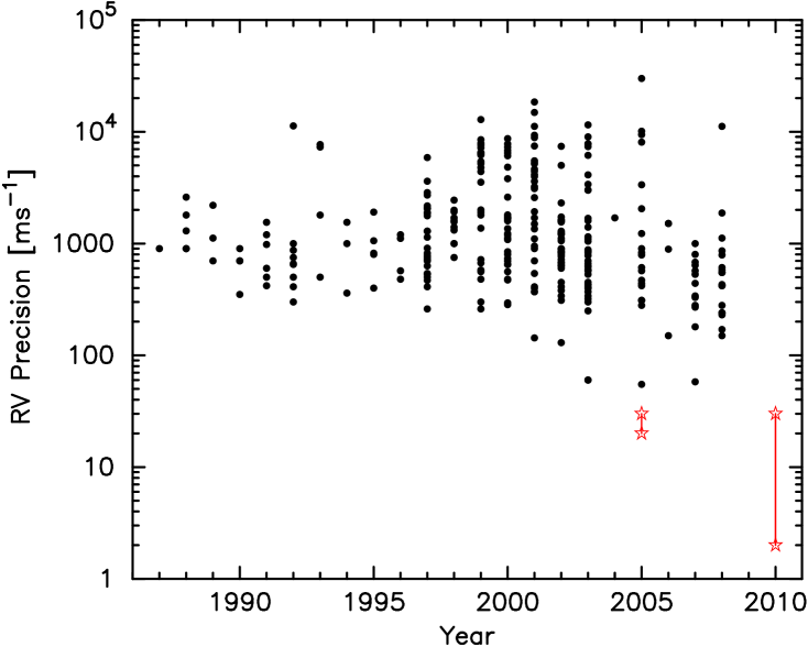
Figure 1.— Radial velocity precision (an rms from the orbital fit) for the primaries of double-lined spectroscopic binaries as a function of the publication date based on the ninth catalogue of spectroscopic binary orbits (Pourbaix et al., 2004). It is worth noting that already in the early XX century an RV precision of several km s^-1 for double-lined binaries was possible (Plummer et al., 1908, HD83808). Current and previous precision range from our method is delimited with the red stars (note the logarithmic scale).

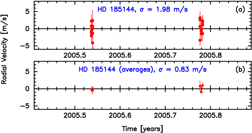
Figure 2.— A series of the precision RV measurements of a single star HD185144 (V=4.7 mag, K0V) taken with the Keck I/HIRES and reduced using our iodine cell data pipeline. The data were taken on 5 nights: two in July (5 consecutive spectra each night) and three in October 2005 (four consecutive spectra each night). The average SNR was 600 for the template exposure as well as for all the spectra taken with the iodine cell.

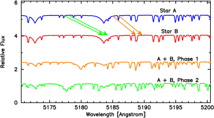
Figure 3.— An SB2 as nature’s realization of the tomographic imaging. The composite spectrum of an SB2 taken at any orbital phase can be interpreted as a result of imaging of a two-layered object. By observing an SB2 at several different orbital phases and hence different RVs of its components, one can carry out an equivalent of tomographic imaging and eventually be able to disentangle the component (“layer”) spectra.

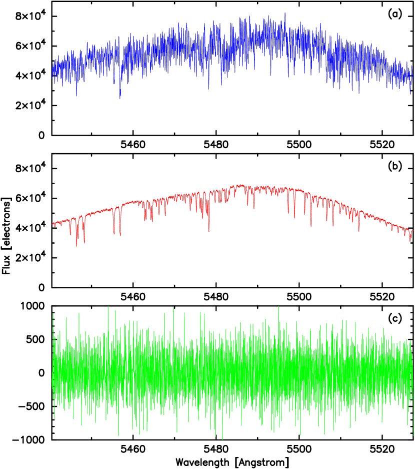
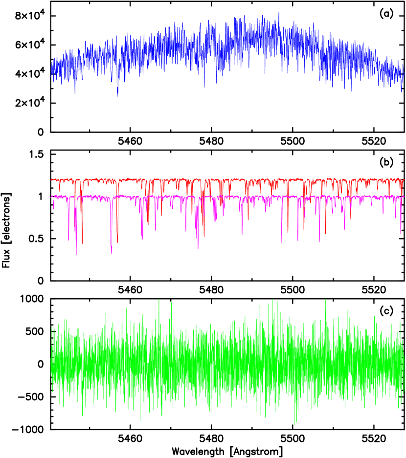
Figure 4.— Left and right (a): a piece of a spectrum of HD4676 as a function of wavelength as seen through an iodine cell. Left (b): a template composite spectrum of HD4676 taken just after the iodine cell exposure shown in (a). Right (b): the corresponding continuum normalized disentangled component spectra of HD4676 shifted accordingly to their respective RVs. Left and right (c): the residuals after subtracting (b) from (a) and accounting for the iodine cell lines. The residuals from the disentangled component spectra are smaller than from the observed composite spectrum.

Figure 5.— Radial velocity variations due to tidal distortion of the binary components as a function of the orbital phase for HD78418 (a), HD123999 (b), HD160922(c), HD200077 (d) and HD210027 (e). The solid line is for the primary and the dashed-dotted line for the secondary.

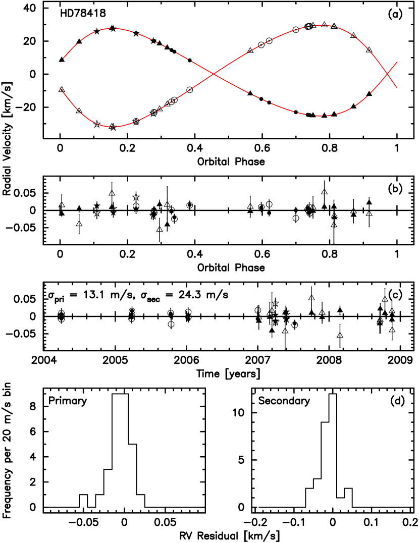
Figure 6.— Observed and modelled radial velocities of HD78418 as a function of the orbital phase (a), their best-fit residuals as a function of the orbital phase (b) and time (c). The histograms of the residuals for the primary and secondary (d). The Keck I/Hires is denoted with circles, Shane/CAT/Hamspec with triangles and TNG/Sarg with stars.

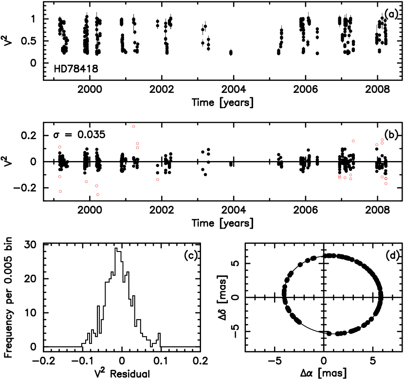
Figure 7.— Visibility measurements of HD78418 as a function of time (a), their best-fit residuals as a function of time (b) and histogram (c). The measurements used to determine the best-fit orbital solution are denoted with filled circles. The corresponding orbital coverage and the relative orbit is shown in the panel (d).

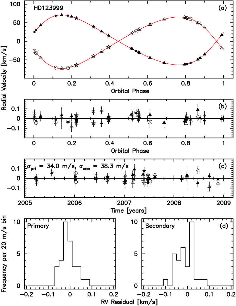
Figure 8.— Observed and modelled radial velocities of HD123999 as a function of the orbital phase (a), their best-fit residuals as a function of the orbital phase (b) and time (c). The histograms of the residuals for the primary and secondary (d). The Keck I/Hires is denoted with circles, Shane/CAT/Hamspec with triangles and TNG/Sarg with stars.

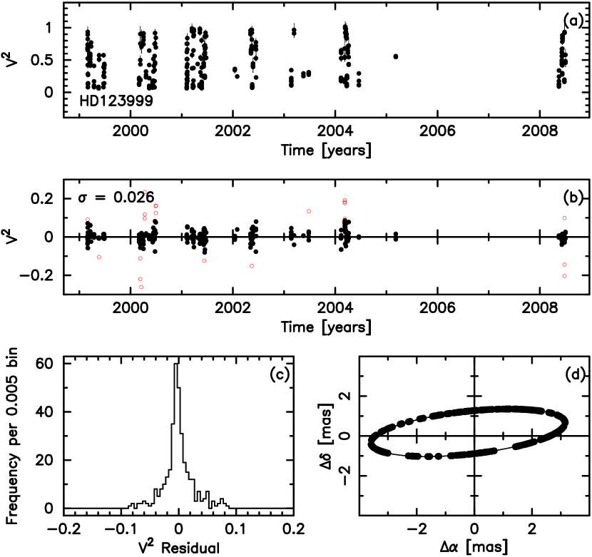
Figure 9.— Visibility measurements of HD123999 as a function of time (a), their best-fit residuals as a function of time (b) and histogram (c). The measurements used to determine the best-fit orbital solution are denoted with filled circles. The corresponding orbital coverage and the relative orbit is shown in the panel (d).

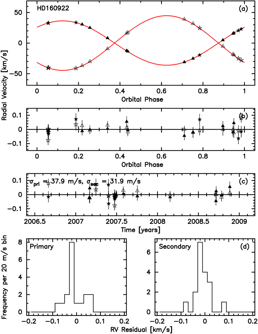
Figure 10.— Observed and modelled radial velocities of HD160922 as a function of the orbital phase (a), their best-fit residuals as a function of the orbital phase (b) and time (c). The histograms of the residuals for the primary and secondary (d). The Keck I/Hires is denoted with circles, Shane/CAT/Hamspec with triangles and TNG/Sarg with stars.

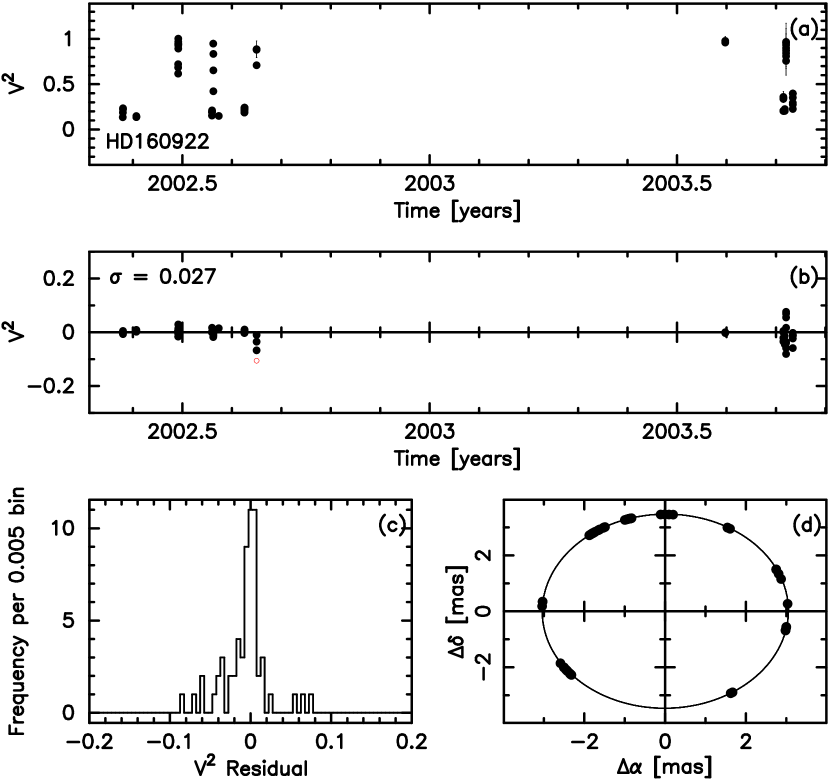
Figure 11.— Visibility measurements of HD160922 as a function of time (a), their best-fit residuals as a function of time (b) and histogram (c). The measurements used to determine the best-fit orbital solution are denoted with filled circles. The corresponding orbital coverage and the relative orbit is shown in the panel (d).

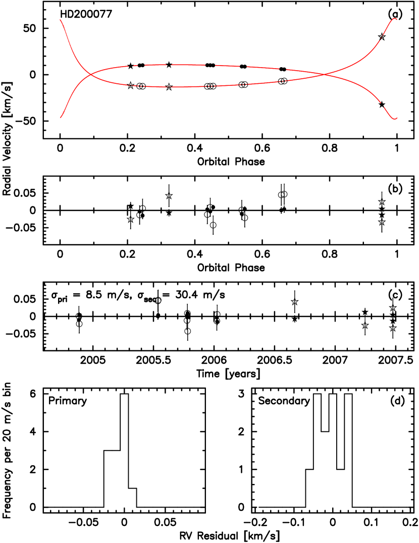
Figure 12.— Observed and modelled radial velocities of HD200077 as a function of the orbital phase (a), their best-fit residuals as a function of the orbital phase (b) and time (c). The histograms of the residuals for the primary and secondary (d). The Keck I/Hires is denoted with circles, Shane/CAT/Hamspec with triangles and TNG/Sarg with stars.

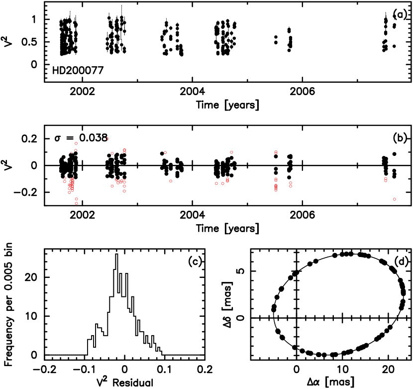
Figure 13.— Visibility measurements of HD200077 as a function of time (a), their best-fit residuals as a function of time (b) and histogram (c). The measurements used to determine the best-fit orbital solution are denoted with filled circles. The corresponding orbital coverage and the relative orbit is shown in the panel (d).

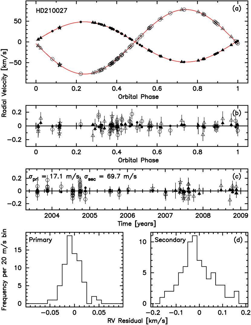
Figure 14.— Observed and modelled radial velocities of HD210027 as a function of the orbital phase (a), their best-fit residuals as a function of the orbital phase (b) and time (c). The histograms of the residuals for the primary and secondary (d). The Keck I/Hires is denoted with circles, Shane/CAT/Hamspec with triangles and TNG/Sarg with stars.

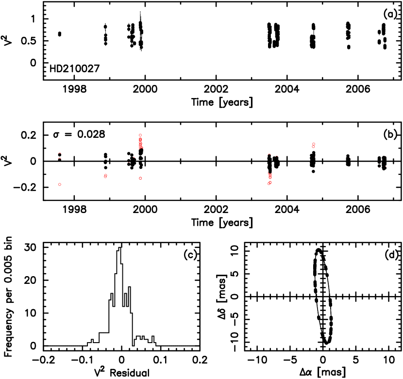
Figure 15.— Visibility measurements of HD210027 as a function of time (a), their best-fit residuals as a function of time (b) and histogram (c). The measurements used to determine the best-fit orbital solution are denoted with filled circles. The corresponding orbital coverage and the relative orbit is shown in the panel (d).

Figure 16.— The isochrones in the mass - absolute magnitude plane for HD78418 (top), HD123999 (middle) and HD160922 (bottom) together with the corresponding best-fitting isochrones.

Figure 17.— The isochrones in the mass - absolute magnitude plane for HD200077 (top two panels) and HD210027 (bottom four panels) together with the corresponding best-fitting isochrones. In the case of HD210027 their companions are shown separately so as it is easier to compare the errorbars with the isochrones.

Figure 18.— Circumbinary planet detection limits in the log P - log M space (orbital period -mass; left panels) and periodograms (right panels). The solid horizontal line in the right panels is a planet detection limit corresponding to the 99% confidence level. The vertical line near the orbital period of 1000 days denotes the time span of the data set. The first stable planetary orbits have the periods of respectively 38, 20 and 890 days as calculated based on Holman & Wiegert (1999)

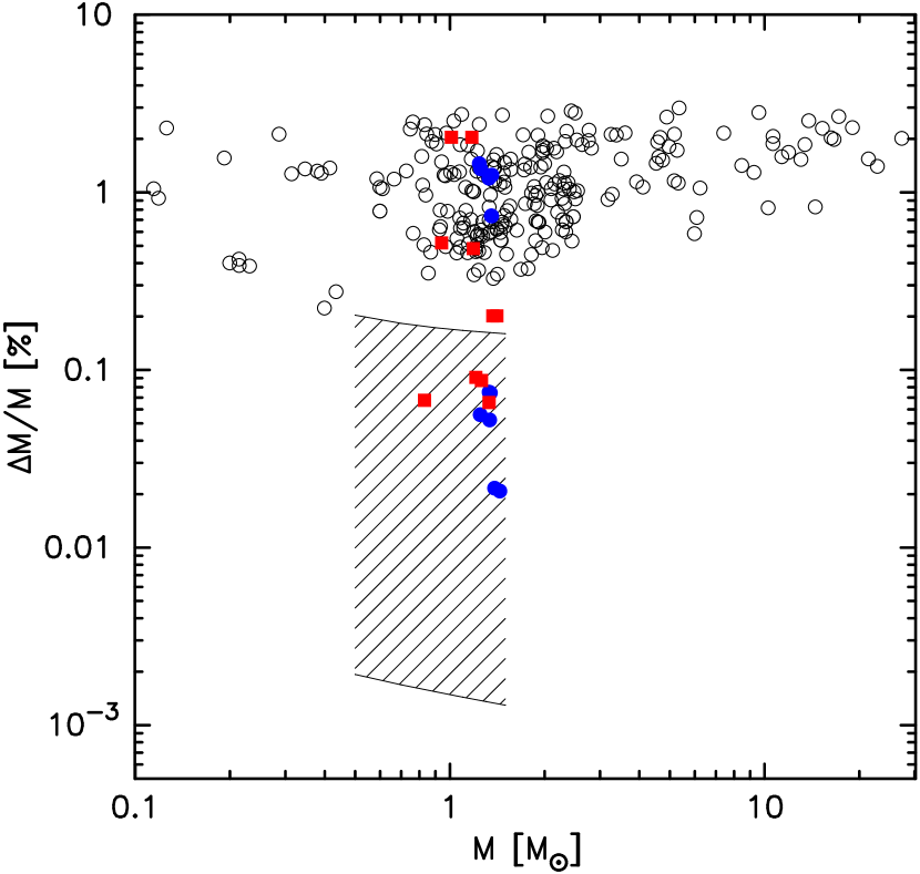
Figure 19.— Fractional accuracy in masses for the binary stars with the most accurate mass determinations in the literature. Open circles denote the binaries from a recent review by Torres et al. (2009). Filled (blue) circles denote the double neutron star systems B1913+16, B2127+11C, B1534+12, J0737-3039, J1756-2251 and J1906+0746 characterized with radio pulsar timing (Nice et al., 2008). Filled (red) rectangles denote the masses for HD78418, HD123999, HD200077 and HD210027 from this paper and a mass determination for AI Phe from our recent work (Hełminiak et al., 2009). The hatched area is the expected precision in masses for double-lined eclipsing binary stars assuming a mass range of the components of 0.5-1.5 M_⊙, orbital period range of 3-23 days, orbital inclination range of 85-90^∘, inclination’s error range of 0.05-0.3^∘ and radial velocity amplitudes’ error range of 1-31 m s^-1.

Table 1Radial velocities of HD78418, HD123999, HD160922, HD200077 and HD210027

Target	Time	RV1	$\sigma_{1}$	O-C1	$\epsilon_{1}$	RV2	$\sigma_{2}$	O-C2	$\epsilon_{2}$	Inst.
	(TDB-2400000.5)	(km s-1)	(km s-1)	(km s-1)	(km s-1)	(km s-1)	(km s-1)	(km s-1)
HD78418	53094.347119	-14.83066	0.00854	0.00538	0.00299	38.51581	0.01243	0.00234	0.00580	HO
	53094.395761	-14.91605	0.01039	0.00241	0.00663	38.60908	0.01267	-0.00023	0.00628	HO
	…
	54101.570433	-7.42109	0.00876	-0.00731	0.00357	29.91678	0.01302	0.01759	0.00697	HN
	53744.479316	34.57326	0.00817	0.00352	0.00167	-18.81645	0.01216	0.01278	0.00518	HN
	…
	54788.464774	18.30307	0.00696	-0.00953	0.00485	0.16661	0.03029	0.01501	0.01374	H
	54430.494032	-2.05150	0.00974	-0.00216	0.00836	23.77923	0.03049	0.01071	0.01416	H
	…
	54190.964445	34.26932	0.01290	0.00397	0.01290	-19.07279	0.01534	0.03793	0.01534	S
	54191.956955	29.78440	0.01249	-0.01327	0.01249	-13.94505	0.01050	-0.01623	0.01050	S
HD123999	53454.573974	-51.41296	0.03155	0.00976	0.00585	72.66300	0.03675	0.00268	0.01119	HN
	53456.545316	39.94170	0.03231	-0.02204	0.00911	-21.65504	0.03623	-0.04321	0.00937	HN
	…
	53978.858598	24.88006	0.04693	0.00628	0.03523	-6.43652	0.03679	-0.01637	0.03679	S
	54247.021370	48.74097	0.03697	0.07561	0.02015	-31.00316	0.03535	-0.04846	0.03535	S
	…
	54107.560803	-52.70193	0.02118	-0.02634	0.01388	73.95953	0.03339	-0.02783	0.01819	H
	54108.572117	-25.53836	0.04058	-0.01830	0.03730	45.98819	0.05134	0.02694	0.04303	H

Note. — $\sigma_{1,2}$ denote the total errors used in the least-squares fits and $\epsilon_{1,2}$ denote the internal errors. The last column denotes the spectrograph used to obtain a measurement. HN stands for Keck I/Hires with the upgraded detector, HO with the old detector, S stands for TNG/Sarg and H for Shane/CAT/Hamspec. The rest of this data set and the other RV sets are available via the link to the machine-readable version.

Table 2Assumed Parameters for HD78418, HD123999, HD160922, HD200077 and HD210027

Parameter	HD78418	HD123999	HD160922	HD200077	HD210027
Eff. temperature, primary, $T_{1}$ (K)	6000	6130	6500	6000	6642
Eff. temperature, secondary, $T_{2}$ (K)	5900	6230	5900	5500	4991
Potential, primary, $\Omega_{1}$	27.1	12.03	14.3	26.7	20.0
Potential, secondary, $\Omega_{2}$	34.9	15.21	14.1	26.5	22.5
Synchronization factor, primary, $F_{1}$	1.51	1.5	1.0	6.57	1.0
Synchronization factor, secondary, $F_{2}$	1.51	1.5	1.0	6.57	1.0
Gravity darkening exponent, primary, $g_{1}$	0.4	0.35	0.3	0.35	0.3
Gravity darkening exponent, secondary, $g_{2}$	0.4	0.35	0.3	0.4	0.4
Albedo, primary, $A_{1}$	0.5	0.5	0.5	0.5	0.5
Albedo, secondary, $A_{2}$	0.5	0.5	0.5	0.5	0.5
Metallicity	-0.09	0.0	0.0	-0.14	0.0
Apparent diameter, primary, $\theta_{1}$ (mas)	0.45	0.638	0.5	0.26	1.06
Apparent diameter, secondary, $\theta_{2}$ (mas)	0.30	0.480	0.4	0.21	0.6

Table 3Calibration stars for visibility measurements of HD78418, HD123999, HD160922, HD200077 and HD210027

Target	Calibrator	Spectral	Magnitude	Angular Separation	Apparent
		Type		from Target (deg)	Diameter (mas)
HD78418
	HD79452	G6III	6.0 V, 3.8 K	8.1	0.79
	HD73192	K2III	6.0 V, 3.3 K	9.0	1.38
HD123999
	HD121107	G5III	5.7 V, 3.6 K	8.2	0.70
	HD128167	F3V	4.5 V, 3.6 K	7.1	0.79
	HD123612	K5III	6.6 V, 3.0 K	0.9	1.29
HD160922
	HD154633	G5V	6.1 V, 4.5 K	5.4	0.31
	HD158633	K0V	6.4 V, 4.4 K	1.8	0.59
	HD168151	F5V	5.0 V, 3.9 K	5.7	0.56
HD200077
	HD192640	A2V	4.9 V, 4.9 K	9.5	0.71
	HD192985	F5V	5.9 V, 4.8 K	9.6	0.39
	HD199763	G9III	6.5 V, 4.3 K	9.9	0.78
HD210027
	HD211006	K2III	5.9 V, 3.2 K	3.6	1.06
	HD211432	G9III	6.4 V, 4.2 K	3.2	0.70
	HD215510	G6III	6.3 V, 4.2 K	10.7	0.85
	HD210459	F5III	4.3 V, 2.5 K	7.9	0.81

Table 4Best-fit Orbital Solutions for HD78418, HD123999, HD160922, HD200077 and HD210027

Parameter	HD78418	HD123999	HD160922	HD200077	HD210027
Apparent semi-major axis, $\hat{a}$ (mas)	5.8696(96)	3.4706(55)	3.469(17)	14.453(18)	10.329(16)
Period, $P$ (d)	19.412347(23)	9.6045601(36)	5.2797766(44)	112.5131(14)	10.2130253(16)
Time of periastron, $T_{p}$ (TDB-2400000.5)	53895.4025(24)	54099.93572(70)	54348.583(83)	53830.168(14)	52997.378(52)
Eccentricity, $e$	0.19494(11)	0.19214(15)	0.00220(31)	0.66227(51)	0.001764(63)
Longitude of the periastron, $\omega$ (deg)	283.389(39)	286.832(29)	314.8(5.6)	197.071(25)	272.8(1.8)
Longitude of the ascending node, $\Omega$ (deg)	171.892(85)	80.49(10)	1.23(32)	89.403(28)	176.262(75)
Inclination, $i$ (deg)	146.88(25)	107.95(12)	151.4(1.1)	118.681(80)	95.83(12)
Magnitude difference (K band), $\Delta K$	1.1445(131)	0.601(13)	0.841(18)	1.1968(88)	1.675(15)
Magnitude difference (H band), $\Delta H$	1.1726(349)	0.667(30)	…	1.263(38)	1.75(11)
Velocity amplitude of the primary, $K_{1}$ (km s-1)	26.4961(35)	67.189(11)	36.254(16)	29.373(82)	48.4757(39)
Velocity amplitude of the secondary, $K_{2}$ (km s-1)	30.7579(65)	69.311(14)	44.720(16)	37.03(11)	77.777(16)
Gamma velocity, $V_{R}$ (km s-1)	9.7478(60)	9.646(13)	-14.011(19)	-36.009(18)	-4.6504(34)

Table 5Various Fit Parameters for HD78418, HD123999, HD160922, HD200077 and HD210027

Parameter	HD78418	HD123999	HD160922	HD200077	HD210027
Velocity offsets
Secondary vs primary (km s-1)	0.239(12)	0.032(21)	0.116(29)	0.340(42)	0.333(16)
Hires old vs new detector, primary, $v_{11}$ (km s-1)	-0.0009(71)	…	…	…	-0.0053(38)
Hires old vs new detector, secondary, $v_{12}$ (km s-1)	-0.0131(11)	…	…	…	0.003(21)
Hamspec vs Hires new detector, primary, $v_{21}$ (km s-1)	0.0358(67)	-0.010(15)	…	…	-0.0141(68)
Hamspec vs Hires new detector, secondary, $v_{22}$ (km s-1)	0.054(12)	0.042(18)	…	…	0.026(27)
Sarg vs Hires new detector, primary, $v_{31}$ (km s-1)	-0.3059(87)	-0.182(24)	…	-0.3092(79)	-0.3026(93)
Sarg vs Hires new detector, secondary, $v_{32}$ (km s-1)	-0.286(10)	-0.151(25)	…	-0.229(23)	-0.256(32)
Hamspec vs Sarg, primary, $v_{41}$ (km s-1)	…	…	0.262(21)	…	…
Hamspec vs Sarg, secondary, $v_{42}$ (km s-1)	…	…	0.344(21)	…	…
Least-squares fit parameters
Number of RV measurements, total	58	64	36	26	144
Number of RV measurements, Keck/Hires	26	16	…	18	102
Number of RV measurements, Shane/CAT/Hamspec	24	34	20	…	30
Number of RV measurements, TNG/Sarg	8	14	16	8	12
Number of V2 measurements	415	346	61	329	266
Additional RV error, Keck/Hires, primary/secondary (m s-1)	8.0/11.0	31.0/35.0	…	5.0/26.0	10.5/65.0
Additional RV error, Shane/CAT/Hamspec, primary/secondary (m s-1)	5.0/27.0	16.0/28.0	27.0/15.0	…	18.5/68.0
Additional RV error, TNG/Sarg, primary/secondary (m s-1)	0.0/0.0	31.0/0.0	37.0/25.0	0.0/26.0	10.5/38.0
Combined RV rms, primary/secondary (m s-1)	13.1/24.3	34.0/38.3	37.9/31.9	8.5/30.4	17.1/69.7
Keck/Hires RV rms, primary/secondary (m s-1)	6.9/14.3	30.2/35.8	…	6.7/17.1	14.1/64.6
Shane/CAT/Hamspec RV rms, primary/secondary (m s-1)	18.2/33.8	36.3/37.6	25.6/14.8	…	22.7/84.2
TNG/Sarg RV rms, primary/secondary (m s-1)	8.2/17.4	40.2/26.8	35.9/37.1	10.4/25.9	12.3/55.8
V2 rms	0.0351	0.0261	0.0274	0.0381	0.0281
RV $\chi^{2}$, primary/secondary	31.60/32.99	28.21/28.20	19.31/18.19	11.28/13.41	70.40/64.94
V2 $\chi^{2}$	433.71	482.46	50.59	522.01	248.29
Degrees of freedom, $DOF$	454	393	83	355	391
Total reduced $\chi^{2}$, $\chi^{2}/DOF$	1.096	1.371	1.061	1.608	0.981

Table 6Physical Parameters for HD78418, HD123999, HD160922, HD200077 and HD210027

Star	Parameter	Primary	Secondary
HD78418	Semi-major axis, $a_{1,2}$ (AU)	0.084874(11)	0.098526(21)
	M $\sin^{3}i$ (M⊙)	0.191350(50)	0.164836(45)
	Mass, $M$ (M⊙)	1.173(24)	1.011(21)
	MK,2MASS (mag)	2.223(16)	3.367(18)
	MH,2MASS (mag)	2.397(37)	3.570(45)
	Parallax, $\kappa$ (mas)		32.004(52)
	Distance, $d$ (pc)		31.246(51)
HD123999	Semi-major axis, $a_{1,2}$ (AU)	0.061193(10)	0.063125(13)
	M $\sin^{3}i$ (M⊙)	1.21467(33)	1.17749(33)
	Mass, $M$ (M⊙)	1.4109(28)	1.3677(28)
	MK,2MASS (mag)	1.254(18)	1.855(19)
	MH,2MASS (mag)	1.314(20)	1.981(26)
	Parallax, $\kappa$ (mas)		27.917(44)
	Distance, $d$ (pc)		35.820(57)
HD160922	Semi-major axis, $a_{1,2}$ (AU)	0.036728(16)	0.045306(17)
	M $\sin^{3}i$ (M⊙)	0.160409(88)	0.130039(80)
	Mass, $M$ (M⊙)	1.46(16)	1.18(13)
	MK,2MASS (mag)	2.16(25)	3.00(25)
	MH,2MASS (mag)	…	…
	Parallax, $\kappa$ (mas)		42.29(27)
	Distance, $d$ (pc)		23.65(15)
HD200077	Semi-major axis, $a_{1,2}$ (AU)	0.25945(74)	0.32711(96)
	M $\sin^{3}i$ (M⊙)	0.8008(34)	0.6352(30)
	Mass, $M$ (M⊙)	1.1860(57)	0.9407(49)
	MK,2MASS (mag)	2.389(24)	3.585(25)
	MH,2MASS (mag)	2.412(23)	3.675(36)
	Parallax, $\kappa$ (mas)		24.640(32)
	Distance, $d$ (pc)		40.571(52)
HD210027	Semi-major axis, $a_{1,2}$ (AU)	0.0457446(37)	0.073395(15)
	M $\sin^{3}i$ (M⊙)	1.31190(29)	0.81767(22)
	Mass, $M$ (M⊙)	1.33249(86)	0.83050(55)
	MK,2MASS (mag)	2.5125(70)	4.187(14)
	MH,2MASS (mag)	2.606(19)	4.353(89)
	Parallax, $\kappa$ (mas)		86.70(14)
	Distance, $d$ (pc)		11.534(19)

References

- Bagnuolo & Gies (1991) Bagnuolo, W. G., Jr., & Gies, D. R. 1991, ApJ, 376, 266
- Boden et al. (2005) Boden, A. F., Torres, G., & Hummel, C. A. 2005, ApJ, 627, 464
- Boden et al. (2000a) Boden, A. F., Creech-Eakman, M. J., & Queloz, D. 2000a, ApJ, 536, 880
- Boden (2000b) Boden, A. F. 2000b, Principles of Long Baseline Stellar Interferometry, 9
- Boden et al. (1999) Boden, A. F., et al. 1999, ApJ, 515, 356
- Boden, Colavita, van Belle, & Shao (1998) Boden, A. F., Colavita, M. M., van Belle, G. T., & Shao, M. 1998, Proc. SPIE, 3350, 872
- Bouchet et al. (1991) Bouchet, P., Schmider, F. X., & Manfroid, J. 1991, A&AS, 91, 409
- Campbell (1898) Campbell, W. W. 1898, ApJ, 8, 123
- Campbell (1900) Campbell, W. W. 1900, ApJ, 11, 259
- Campbell & Curtis (1905) Campbell, W. W., & Curtis, H. D. 1905, Lick Observatory Bulletin, 3, 136
- Campbell et al. (1911) Campbell, W. W., Moore, J. H., Wright, W. H., & Duncan, J. C. 1911, Lick Observatory Bulletin, 6, 140
- Campbell (1916) Campbell, W. W. 1916, Lick Observatory Bulletin, 9, 30
- Colavita et al. (1999a) Colavita, M. M. et al. 1999a, ApJ, 510, 505
- Colavita (1999b) Colavita, M. M. 1999b, PASP, 111, 111
- de Medeiros & Udry (1999) de Medeiros, J. R., & Udry, S. 1999, A&A, 346, 532
- Eaton (2008) Eaton, J. A. 2008, ApJ, 681, 562
- Endl et al. (2000) Endl, M., Kürster, M., & Els, S. 2000, A&A, 362, 585
- Fekel et al. (2009) Fekel, F. C., Tomkin, J., & Williamson, M. H. 2009, AJ, 137, 3900
- Fekel & Tomkin (1983) Fekel, F. C., & Tomkin, J. 1983, PASP, 95, 1000
- Goldberg et al. (2002) Goldberg, D., Mazeh, T., Latham, D. W., Stefanik, R. P., Carney, B. W., & Laird, J. B. 2002, AJ, 124, 1132
- Hełminiak et al. (2009) Hełminiak, K. G., Konacki, M., Ratajczak, M., & Muterspaugh, M. 2009, arXiv:0908.3471
- Holman & Wiegert (1999) Holman, M. J., & Wiegert, P. A. 1999, AJ, 117
- Kamp (1967) van de Kamp, P. 1967, Principles of Astrometry, Freeman, San Francisco
- Kaplan et al. (1989) Kaplan, G. H., Hughes, J. A., Seidelmann, P. K., Smith, C. A., & Yallop, B. D. 1989, AJ, 97, 1197
- Konacki (2005) Konacki, M. 2005a, ApJ, 626, 431
- Konacki & Lane (2004) Konacki, M., & Lane, B. F. 2004, ApJ, 610, 443
- Konacki (2009a) Konacki, M. 2009a, IAU Symposium, 253, 141
- Konacki et al. (2009b) Konacki, M., Muterspaugh, M. W., Kulkarni, S. R., & Hełminiak, K. G. 2009b, ApJ, 704, 513
- Kopal (1980) Kopal, Z. 1980, Ap&SS, 70, 329
- Kopeikin & Ozernoy (1999) Kopeikin, S. M., & Ozernoy, L. M. 1999, ApJ, 523, 771
- Kurucz (1995) Kurucz, R. L. 1995, ASP Conf. Ser. 78: Astrophysical Applications of Powerful New Databases, 205
- Kovalevsky (1995) Kovalevsky, J. 1995, Modern Astrometry, Springer-Verlag Berlin Heidelberg New York, Astronomy and Astrophysics Library
- Lane & Boden (1999) Lane, B. F., & Boden, A. F. 1999, Working on the Fringe: Optical and IR Interferometry from Ground and Space, 194, 51
- Marcy & Butler (1992) Marcy, G. W. & Butler, R. P. 1992, PASP, 104, 270
- Marigo et al. (2008) Marigo, P., Girardi, L., Bressan, A., Groenewegen, M. A. T., Silva, L., & Granato, G. L. 2008, A&A, 482, 883
- Mazeh (2008) Mazeh, T. 2008, EAS Publications Series, 29, 1
- Morel et al. (2000) Morel, P., Morel, C., Provost, J., & Berthomieu, G. 2000, A&A, 354, 636
- Mozurkewich et al. (1991) Mozurkewich, D. et al. 1991, AJ, 101, 2207
- Nice et al. (2008) Nice, D. J., Stairs, I. H., & Kasian, L. E. 2008, 40 Years of Pulsars: Millisecond Pulsars, Magnetars and More, 983, 453
- Nordström et al. (2008) Nordström, B., et al. 2008, VizieR Online Data Catalog, 5117, 0
- Nordström et al. (2004) Nordström, B., et al. 2004, A&A, 418, 989
- Pickering (1890) Pickering, E. C. 1890, The Observatory, 13, 80
- Plummer et al. (1908) Plummer, H. C. K., Wright, W. H., & Turner, A. B. 1908, Lick Observatory Bulletin, 5, 21
- Pourbaix et al. (2004) Pourbaix, D., et al. 2004, A&A, 424, 727
- Skrutskie et al. (2006) Skrutskie, M. F., et al. 2006, AJ, 131, 1163
- Sterne (1941) Sterne, T. E. 1941, Proceedings of the National Academy of Science, 27, 168
- Tomkin & Fekel (2006) Tomkin, J., & Fekel, F. C. 2006, AJ, 131, 2652
- Torres et al. (2009) Torres, G., Andersen, J., & Gimenez, A. 2009, arXiv:0908.2624
- Valenti et al. (1995) Valenti, J. A., Butler, R. P., & Marcy, G. W. 1995, PASP, 107, 966
- Vogel (1890a) Vogel, H. C. 1890a, Astronomische Nachrichten, 123, 289
- Vogel (1890b) Vogel, H. C. 1890b, PASP, 2, 27
- Vogel (1890c) Vogel, H. C. 1890c, MNRAS, 50, 239
- Vogel (1891) Vogel, H. C. 1891, MNRAS, 52, 87
- Vogel (1900) Vogel, H. C. 1900, ApJ, 11, 393
- Wilson (1979) Wilson, R. E. 1979, ApJ, 234, 1054
- Wilson & Sofia (1976) Wilson, R. E., & Sofia, S. 1976, ApJ, 203, 182
- Wilson & Devinney (1971) Wilson, R. E., & Devinney, E. J. 1971, ApJ, 166, 605
- Zucker & Mazeh (1994) Zucker, S. & Mazeh, T. 1994, ApJ, 420, 806
- Zucker & Alexander (2007) Zucker, S., & Alexander, T. 2007, ApJ, 654, L83