Fluctuations in Gene Regulatory Networks as Gaussian Colored Noise

Abstract

The study of fluctuations in gene regulatory networks is extended to the case of Gaussian colored noise. Firstly, the solution of the corresponding Langevin equation with colored noise is expressed in terms of an Ito integral. Then, two important lemmas concerning the variance of an Ito integral and the covariance of two Ito integrals are shown. Based on the lemmas, we give the general formulae for the variances and covariance of molecular concentrations for a regulatory network near a stable equilibrium explicitly. Two examples, the gene auto-regulatory network and the toggle switch, are presented in details. In general, it is found that the finite correlation time of noise reduces the fluctuations and enhances the correlation between the fluctuations of the molecular components.

I Introduction

A regulatory network of gene expression consists of a group of genes which co-regulate one another’s expression. The networks provide a fundamental description of cellular function that is the subject of the recently emerged field of systems biology alon . The advance of experimental techniques in constructing synthetic networks provided with the basic elements, such as a switch ptashne ; hasty ; gardner and an oscillator elowitz ; atkinson , for the design of biological circuits alon . For such elements, the characteristic features are determined mainly by the regulation scheme, and fluctuations always appear to be significant due to low copy numbers of molecules and stochastic nature of biochemical reactions rao ; pedraza . In clarifying the nature of regulation mechanism, one of the important questions is to understand the way of accommodating the fluctuations meanwhile maintaining the stability for a genetic network. Recently, significant progress has been made along this aspect. One of the noticeable examples is the auto-regulatory network of a single gene for which, the protein encoded in the gene serves as the regulator of itself through either negative or positive feedback. Such autoregulation is an ubiquitous motif in biochemical pathways alon . It was demonstrated by Becskei and Serrano that an autoregulatory network with negative feedback may gain stability becskei . Further analysis given by Thattai and van Oudenaarden thattai and by Ozbudak et al. ozbudak indicate that noise is essentially determined at the translational level and negative feedback can suppress the intrinsic noise. Another example is the genetic toggle switch. Such a switch consists of two transcription factors which regulate each other’s synthesis negatively gardner . Detailed analysis given by Cherry and Adler cherry shows that the cooperative binding of two or more proteins in negative regulation is required, in general, for a switch to have two distinct stable states. Further study carried out by Warren and ten Wolde warren indicates that the switch stability can be enhanced by overlapping the upperstream regulatory domains such that competing regulatory molecules mutually exclude each other, and robustness against biochemical noise may provide a selection pressure that drives operons together in the course of evolution. Recently, the results reported by Loinger et al loinger reveal that a suitable combination of network structure and stochastic effects gives rise to bistability even without cooperative binding.

Stochastic fluctuations associated with a system are often assumed to be Gaussian white noise in nature. However, the zero correlation time for white noise assumes an infinite relaxation time. Thus, it is important to incorporate the effect of finite correlation time of noise into the study of stochastic fluctuations. As the treatment for the effect induced by the Gaussian colored noise in a regulatory network being still lacking in the literature, we intend to fill up this gap in this paper. In modelling the dynamics of a regulatory network, rate-equation approach is often used; the approach reflects the macroscopic observation of deterministic nature. Noise-induced effects may be incorporated into the framework by employing the master equation and then proceeding via stochastic Monte Carlo simulations gillespie as was done for the first time for gene regulatory networks by Arkin et al arkin . In general, master equations are discrete in nature. By using the technique of $\Omega$-expansion kampen , one can convert a master equation to continuous Fokker-Planck equation which then can be treated analytically by various approximations. Based on the Fokker-Planck equation, Tao and Tao et al. derived the corresponding linear noise Fokker-Planck equation which is suitable for the study of fluctuations caused by the white noise tao ; tao-c . One may include the Gaussian colored noise into the frame of Fokker-Planck equation by using the scheme of unified colored-noise approximation jung or via kinetic Monte-Carlo simulations as was implemented for gene regulatory networks in shahrezaei . Alternatively, we first establish the equivalent Langevin description for a system with colored noise in the linearized region of a stable point gardiner . The solution of the corresponding Langevin equation is given in the form of an Ito integral, and the fluctuations of molecular concentrations then can be evaluated by using the two lemmas, which concern with the variances and covariances of Ito integrals, shown in this work. As the correlation time of noise is set to vanish, we recover the results of fluctuations for white noise. Based on this approach, we analyze the stochastic fluctuations of autoregulatory networks and toggle switches with general cooperative binding, and the results are found to be in good agreement with those obtained from numerical simulations. In general, the appearance of finite correlation time of noise decreases the fluctuations of a system and enhances the correlation between fluctuations.

This paper is organized as follows. In section II, we first set up the model system for the study of the steady-state statistics of a regulatory network near a stable equilibrium. The rate equations are first linearized about the stable equilibrium. Starting with the rate equations, we then use the technique of $\Omega$-expansion to obtain the corresponding Fokker-Planck equation of the system. In section III, the equivalent Langevin description of the Fokker-Planck equation is given, and the solution of the Langevin equation with colored noise is expressed in terms of an Ito integral. Then, two important lemmas concerning the variance of an Ito integral and the covariance of two Ito integrals are shown. Based on the lemmas, we obtain the variances and covariance of molecular concentrations for a two-dimensional regulatory network near a stable equilibrium. In sections IV, the formulae resulting from the lemmas are applied to auto-regulatory networks and toggle switches to study the stochastic fluctuations of the systems. The comparison between the results and numerical simulations is given. In particular, the effects of noise correlation time on the amount of fluctuations and on the correlation between the two molecular components are analyzed. Finally, we summarize the results in section V.

II Fokker-Planck equation

Consider a two-dimensional regulatory network of gene expression defined by the macroscopic rate equation,

$$dx\left(t\right)=f\left(x\right)dt,$$ (1)

where the state variables $x^{\tau}\left(t\right)=\left(x_{1}\left(t\right),x_{2}\left(t\right)\right)$ are molecular concentrations, and the forces $f^{\tau}\left(x\right)=\left(f_{1}\left(x\right),f_{2}\left(x\right)\right)$ determine the time evolutions of the state variables. Here, the superscript $\tau$ denotes the transpose of a vector. A stable point $x^{\ast}$, specified by zero force $f\left(x^{\ast}\right)=0$, represents a stable stationary state. For the region near the stable equilibrium, the leading order of the drift force in $x$ gives

$$f\left(y\right)=F\left(x^{\ast}\right)\cdot y,$$ (2)

where the stable point is chosen as the origin, $y=x-x^{\ast}$, in our two-dimensional space, and the elements of $F\left(x^{\ast}\right)$ are defined as $F_{ij}\left(x^{\ast}\right)=\left.\partial f_{i}\left(x\right)/\partial x_{j}\right|_{x=x^{\ast}}$. From now on, we drop the arguments whenever the matrix elements are understood as functions of the equilibrium stable point $x^{\ast}$. The matrix $F$ can be diagonalized by means of the transformation matrix $P$,

$$F=P\cdot\left(\begin{array}[]{cc}-\lambda_{1}&0\\ 0&-\lambda_{2}\end{array}\right)\cdot P^{-1},$$ (3)

where $\lambda_{1},\lambda_{2}>0$ for the stable point, and $\det\left(P\right)=1$. The matrix $P$ is set as

$$P=\left(\begin{array}[]{cc}p_{11}&p_{12}\\ p_{21}&p_{22}\end{array}\right),$$ (4)

and  this gives the inverse as

$$P^{-1}=\left(\begin{array}[]{cc}p_{22}&-p_{12}\\ -p_{21}&p_{11}\end{array}\right).$$ (5)

In general, the drift force of Eq. (1) can be expressed as the sum of two terms,

$$f\left(x\right)=R\left(x\right)-\Theta\cdot x,$$ (6)

where the functions, $R^{\tau}\left(x\right)=\left(R_{1}\left(x\right),R_{2}\left(x\right)\right)$, describe the synthesis or feedback regulation of molecule, and $\Theta$ is a $2\times 2$ constant matrix with the elements given by $\Theta_{ij}=\delta_{ij}\theta^{\left(i\right)}$ with the degradation rate $\theta^{\left(i\right)}$ for molecular concentration $x_{i}$. Since the synthesis or feedback regulation of molecule concentration $x_{i}$ depends only on the concentration of other component, we have $R_{i}\left(x\right)=R_{i}\left(x_{j}\right)$ for $j\neq i$. The stochastic fluctuations can be incorporated into Eq. (1) by means of the master equation approach. For this, we introduce the volume factor $\Omega$ to relate the molecular numbers $n^{\tau}=\left(n_{1}\text{, }n_{2}\right)$ to the concentrations $x^{\tau}=\left(x_{1},x_{2}\right)$ as $n^{\tau}=\Omega x^{\tau}$. In terms of molecular numbers $n$, the corresponding master equation for Eq. (1) with the drift force given by Eq. (6) is

$$\frac{\partial P\left(n,t\right)}{\partial t}=\sum_{i=1}^{2}\left(E_{i+}-1\right)\left[\left(\theta^{\left(i\right)}n_{i}\right)P\left(n,t\right)\right]+\Omega\sum_{i=1}^{2}R_{i}\left(x\right)\left[E_{i-}-1\right]P\left(n,t\right),$$ (7)

where $P\left(n,t\right)$ is the probability distribution, the step operators $E_{i\pm}$ are defined as $E_{i\pm}G\left(n_{i}\right)=G\left(n_{i}\pm 1\right)$ for a function of molecular numbers $G\left(n\right)$, and the fact, $R_{i}\left(x\right)=R_{i}\left(x_{j}\right)$ for $j\neq i$, is used for the term in the second sum. Then, the technique of $\Omega$-expansion kampen is employed to transfer the discrete process of Eq. (7) to a continuous process described by the Fokker-Planck equation,

$$\frac{\partial\rho\left(x,t\right)}{\partial t}+\nabla\cdot j\left(x,t\right)=0,$$ (8)

where $\left(\nabla\right)^{\tau}=\left(\partial/\partial x_{1}\text{, }\partial/\partial x_{2}\right)$, $\rho\left(x,t\right)$ is the distribution density, and $j\left(x,t\right)$ is the density current given as

$$j\left(x,t\right)=f\left(x\right)\rho\left(x,t\right)-\left[D\left(x\right)\cdot\nabla\right]\rho\left(x,t\right).$$ (9)

Based on Eq. (7), we obtain the diffusion matrix $D\left(x\right)$ of Eq. (9) as $D_{ij}\left(x\right)=\delta_{ij}d^{\left(i\right)}\left(x\right)$, which takes the diagonal form with the diagonal elements given as

$$d^{\left(i\right)}\left(x\right)=\frac{1}{2\Omega}\left[R_{i}\left(x\right)+\theta^{\left(i\right)}x_{i}\right].$$ (10)

For the linear region specified by Eq. (2) we obtain the corresponding Fokker-Planck equation by expanding the density current $J\left(x,t\right)$ of Eq. (9) around the stable point $x^{\ast}$. The result reads

$$\frac{\partial\rho_{L}\left(y,t\right)}{\partial t}+\nabla\cdot J_{L}\left(y,t\right)=0,$$ (11)

where $J_{L}\left(y,t\right)$ contains only the leading order terms of $J\left(x,t\right)$ in $1/\Omega$,

$$J_{L}\left(y,t\right)=\left[F\left(x^{\ast}\right)\cdot y-D\left(x^{\ast}\right)\cdot\nabla\right]\rho_{L}\left(y,t\right).$$ (12)

This leads to an Ornstein-Uhlenbeck process kampen ; gardiner ; uhlenbeck in which, the drift force is linear and the diffusion is given by a constant matrix.

III Equivalent Langevin description

For the Fokker-Planck equation of Eq. (11), we have the equivalent Langevin description specified by the stochastic differential equation,

$$dy\left(t\right)=F\cdot y\left(t\right)dt+\eta\left(t\right)dt.$$ (13)

From hereafter the stochastic fluctuations, described by the variables $\eta^{\tau}\left(t\right)=\left(\eta_{1}\left(t\right),\eta_{2}\left(t\right)\right)$, will be assumed to be Gaussian colored noises. The two independent colored noises are specified by the differential equation,

$$d\eta\left(t\right)=-\Gamma\cdot\eta\left(t\right)dt+\Gamma\cdot\Lambda\cdot dW\left(t\right),$$ (14)

where the constant matrices, $\Gamma$ and $\Lambda$, and the vector $dW\left(t\right)$ are defined as follows. The elements of the $\Gamma$ matrix are given as $\Gamma_{ij}=\delta_{ij}\left(1/\tau^{\left(i\right)}\right)$, where $\tau^{\left(i\right)}$ is the correlation time of the noise $\eta_{i}$ and the Kronecker delta $\delta_{i,j}$ is equal to $1$ for $i=j$ and $0$ otherwise. The $\Lambda$ matrix is related to the diffusion matrix evaluated at the stable point, $D=D\left(x^{\ast}\right)$, by $\Lambda\cdot\Lambda=2D$. Based on the form of the diffusion matrix of Eq. (10), we have $\Lambda_{ij}=\delta_{ij}\sqrt{2d^{\left(i\right)}\left(x^{\ast}\right)}$ for the elements of $\Lambda$. Furthermore, the variables $dW^{\tau}\left(t\right)=\left(dw_{1}\left(t\right),dw_{2}\left(t\right)\right)$ describe two independent Wiener processes. By rewriting $dW\left(t\right)\rightarrow\xi\left(t\right)dt$, the conditions, $\left\langle\xi\left(t\right)\right\rangle=0$ and $\left\langle\xi\left(t\right)\xi^{\tau}\left(s\right)\right\rangle=\delta\left(t-s\right)$ with the Dirac delta function $\delta\left(t\right)$, specify the Gaussian white noise.

The solution of Eq. (14) can be expressed in terms of Ito integral as

$$\eta\left(t\right)=\eta\left(0\right)\exp\left(-t\Gamma\right)+\int_{0}^{t}\left[\exp\left(-\left(t-s\right)\Gamma\right)\right]\cdot\Gamma\cdot\Lambda\cdot dW\left(s\right).$$ (15)

This yields the correlation function of the Gaussian colored noise as

$$\left\langle\eta\left(t\right)\eta^{\tau}\left(t^{\prime}\right)\right\rangle=\Gamma\cdot D\exp\left(-\left|t-t^{\prime}\right|\Gamma\right).$$ (16)

Then the solution of Eq. (13) can be written as

$$y\left(t\right)=y\left(0\right)\exp\left(tF\right)+\int_{0}^{t}\left[\exp\left(t-u\right)F\right]\cdot\left\{\eta\left(0\right)\exp\left(-u\Gamma\right)+\int_{0}^{u}\left[\exp\left(-\left(u-s\right)\Gamma\right)\right]\cdot\Gamma\cdot\Lambda\cdot dW\left(s\right)\right\}du.$$ (17)

Since we are interested in the fluctuations around the stable point $x^{\ast}$, only the asymptotic behavior of the solution matters, and we may set the initial condition as $y\left(0\right)=0$ and $\eta\left(0\right)=0$ to obtain

$$y\left(t\right)=\int_{0}^{t}\left[\exp\left(t-u\right)F\right]\cdot\left\{\int_{0}^{u}\left[\exp\left(-\left(u-s\right)\Gamma\right)\right]\cdot\Gamma\cdot\Lambda\cdot dW\left(s\right)\right\}du.$$ (18)

Moreover, the order of the double integrations can be changed properly to yield

$$y\left(t\right)=\int_{0}^{t}\left\{\int_{s}^{t}\left[\exp\left(t-u\right)F\right]\cdot\left[\exp\left(-\left(u-s\right)\Gamma\right)\right]\cdot\Gamma\cdot\Lambda du\right\}\cdot dW\left(s\right).$$ (19)

Thus, the form of the solution, in general, is an Ito integral.

Two important lemmas for the evaluations of variances and covariances of Ito integrals are shown as follows. Consider an Ito integral in the form of

$$I\left(t\right)=\int_{0}^{t}V\left(t,s\right)dw\left(s\right),$$ (20)

for a random Wiener process $dw$. The integral can be expressed as the discrete form,

$$I\left(t\right)=\lim_{N\rightarrow\infty}\sum_{k=0}^{N-1}V\left(t,s_{k}\right)\left[w\left(s_{k+1}\right)-w\left(s_{k}\right)\right],$$ (21)

with $s_{0}=0$ and $s_{k}=k\left(t/N\right)$. This leads to the variance of $I\left(t\right)$ as

$$\sigma^{2}\left[I\left(t\right)\right]=\lim_{N\rightarrow\infty}\sum_{k=0}^{N-1}V^{2}\left(t,s_{k}\right)\sigma^{2}\left[w\left(s_{k+1}\right)-w\left(s_{k}\right)\right].$$ (22)

Here the variance of $I\left(t\right)$ is defined as $\sigma^{2}\left[I\left(t\right)\right]=\left\langle I^{2}\left(t\right)\right\rangle-\left\langle I\left(t\right)\right\rangle^{2}$ with the expectation value $\left\langle\cdot\right\rangle$ taken with respect to the distribution of noise at time $t$. Based on the equality for a Wiener process, $\sigma^{2}\left[w\left(s_{k+1}\right)-w\left(s_{k}\right)\right]=s_{k+1}-s_{k}$, we can express Eq. (22) as the integral form and obtain the first lemma, namely, the variance of $I\left(t\right)$ is

$$\sigma^{2}\left[I\left(t\right)\right]=\int_{0}^{t}V^{2}\left(t,s\right)ds.$$ (23)

The first lemma can be further extended to the case of two dimensions in a straightforward way. Consider the Ito integrals, $J^{\tau}\left(t\right)=\left(J_{1}\left(t\right),J_{2}\left(x\right)\right)$, defined as

$$J\left(t\right)=\int_{0}^{t}M\left(t,s\right)\cdot dW\left(s\right),$$ (24)

where $M\left(t,s\right)$ is a $2\times 2$ matrix,

$$M\left(t,s\right)=\left(\begin{array}[]{cc}m_{11}\left(t,s\right)&m_{12}\left(t,s\right)\\ m_{21}\left(t,s\right)&m_{22}\left(t,s\right)\end{array}\right),$$ (25)

and the two variables $dw_{1}$ and $dw_{2}$ in $dW^{\tau}\left(t\right)=\left(dw_{1}\left(t\right),dw_{2}\left(t\right)\right)$ describe two independent random Wiener processes. Following the first lemma along with the property $\left\langle dW\left(t\right)dW^{\tau}\left(s\right)\right\rangle=\delta\left(t-s\right)dt$, one can show that the variances of $J_{1}\left(t\right)$ and $J_{2}\left(t\right)$ are

$$\sigma^{2}\left[J_{i}\left(t\right)\right]=\int_{0}^{t}\left[m_{i1}^{2}\left(t,s\right)+m_{i2}^{2}\left(t,s\right)\right]ds$$ (26)

for $i=1,2$, and the covariance is

$$E\left[J_{1}\left(t\right)J_{2}\left(t\right)\right]=\int_{0}^{t}\left[m_{11}\left(t,s\right)m_{21}\left(t,s\right)+m_{12}\left(t,s\right)m_{22}\left(t,s\right)\right]ds.$$ (27)

Here the covariance of $J_{1}\left(t\right)$ and $J_{2}\left(t\right)$ is defined as $E\left[J_{1}\left(t\right)J_{2}\left(t\right)\right]=\left\langle J_{1}\left(t\right)J_{2}\left(t\right)\right\rangle-\left\langle J_{1}\left(t\right)\right\rangle\left\langle J_{2}\left(t\right)\right\rangle$. These constitute the second lemma.

The second lemma, Eqs. (26) and (27), with the limit $t\rightarrow\infty$ can be employed directly to determine the variances and covariance of $y\left(t\right)$ of Eq. (19) near the stable equilibrium $y=0$. The results thus obtained are summarized in the following. The variances of $y_{1}$ and $y_{2}$, referred as $\sigma_{1}^{2}$ and $\sigma_{2}^{2}$ respectively, are

$$\sigma_{1}^{2}\left(\tau^{\left(1\right)},\tau^{\left(2\right)}\right)=d^{\left(1\right)}\left[\frac{q_{3}^{2}}{\lambda_{1}c_{11}}+\frac{q_{4}^{2}}{\lambda_{2}c_{21}}-\frac{2q_{3}q_{4}\widetilde{c}_{1}}{\lambda_{1}+\lambda_{2}}\right]+d^{\left(2\right)}\left[\frac{q_{1}^{2}}{\lambda_{1}c_{12}}+\frac{q_{1}^{2}}{\lambda_{2}c_{22}}-\frac{2q_{1}^{2}\widetilde{c}_{2}}{\lambda_{1}+\lambda_{2}}\right],$$ (28)

and

$$\sigma_{2}^{2}\left(\tau^{\left(1\right)},\tau^{\left(2\right)}\right)=d^{\left(1\right)}\left[\frac{q_{2}^{2}}{\lambda_{1}c_{11}}+\frac{q_{2}^{2}}{\lambda_{2}c_{21}}-\frac{2q_{2}^{2}\widetilde{c}_{1}}{\lambda_{1}+\lambda_{2}}\right]+d^{\left(2\right)}\left[\frac{q_{3}^{2}}{\lambda_{2}c_{22}}+\frac{q_{4}^{2}}{\lambda_{1}c_{12}}-\frac{2q_{3}q_{4}\widetilde{c}_{2}}{\lambda_{1}+\lambda_{2}}\right];$$ (29)

and the covariance between $y_{1}$ and $y_{2}$, denoted as $E$, is

$$E\left(\tau^{\left(1\right)},\tau^{\left(2\right)}\right)=d^{\left(1\right)}\left[\frac{q_{2}q_{3}}{\lambda_{1}c_{11}}+\frac{q_{2}q_{4}}{\lambda_{2}c_{21}}-\frac{\left(q_{2}q_{3}+q_{2}q_{4}\right)\widetilde{c}_{1}}{\lambda_{1}+\lambda_{2}}\right]+d^{\left(2\right)}\left[\frac{q_{1}q_{4}}{\lambda_{1}c_{12}}+\frac{q_{1}q_{3}}{\lambda_{2}c_{22}}-\frac{\left(q_{1}q_{3}+q_{1}q_{4}\right)\widetilde{c}_{2}}{\lambda_{1}+\lambda_{2}}\right].$$ (30)

Here, the quantities $q_{i}$ are defined as $q_{1}=p_{11}p_{12}$, $q_{2}=p_{21}p_{22}$, $q_{3}=p_{11}p_{22}$, and $q_{4}=p_{12}p_{21}$ with $p_{ij}$ specified by the transformation matrix $P$ of Eq. (4); and the quantities $\widetilde{c}_{i}$ are $\widetilde{c}_{i}=\left(1/c_{1i}\right)+\left(1/c_{2i}\right)$ with $c_{ij}$ defined as $c_{ij}=\lambda_{i}\tau^{\left(j\right)}+1$; for $i$, $j=1$ and $2$.

The stochastic differential equations specified by Eqs. (13) and (14) reduce to

$$dy\left(t\right)=F\cdot y\left(t\right)dt+\Lambda\cdot dW\left(t\right).$$ (31)

for the case of white noise. Similarly to the case of colored noise, the solution of Eq. (31) can be put in the form of Ito integral, and we obtain the variances and covariance of $y_{1}$ and $y_{2}$ as

$$\sigma_{1}^{\left(0\right)2}=d^{\left(1\right)}\left[\frac{q_{3}^{2}}{\lambda_{1}}+\frac{q_{4}^{2}}{\lambda_{2}}-\frac{4q_{3}q_{4}}{\lambda_{1}+\lambda_{2}}\right]+d^{\left(2\right)}\left[\frac{q_{1}^{2}}{\lambda_{1}}+\frac{q_{1}^{2}}{\lambda_{2}}-\frac{4q_{1}^{2}}{\lambda_{1}+\lambda_{2}}\right],$$ (32)

$$\sigma_{2}^{\left(0\right)2}=d^{\left(1\right)}\left[\frac{q_{2}^{2}}{\lambda_{1}}+\frac{q_{2}^{2}}{\lambda_{2}}-\frac{4q_{2}^{2}}{\lambda_{1}+\lambda_{2}}\right]+d^{\left(2\right)}\left[\frac{q_{3}^{2}}{\lambda_{2}}+\frac{q_{4}^{2}}{\lambda_{1}}-\frac{4q_{3}q_{4}}{\lambda_{1}+\lambda_{2}}\right],$$ (33)

and

$$E^{\left(0\right)}=d^{\left(1\right)}\left[\frac{q_{2}q_{3}}{\lambda_{1}}+\frac{q_{2}q_{4}}{\lambda_{2}}-\frac{2\left(q_{2}q_{3}+q_{2}q_{4}\right)}{\lambda_{1}+\lambda_{2}}\right]+d^{\left(2\right)}\left[\frac{q_{1}q_{4}}{\lambda_{1}c_{12}}+\frac{q_{1}q_{3}}{\lambda_{2}c_{22}}-\frac{2\left(q_{1}q_{3}+q_{1}q_{4}\right)}{\lambda_{1}+\lambda_{2}}\right],$$ (34)

where the superscript $\left(0\right)$ in $\sigma$ and $E$ is used to denote the result of white noise. These are exactly the same as those given by Eqs. (28)-(30) but with $\tau^{\left(1\right)}=\tau^{\left(2\right)}=0$. Following this, by setting either $\tau^{\left(1\right)}=0$ or $\tau^{\left(2\right)}=0$ in Eqs. (28)-(30) we have the results for the case of Gaussian colored noise in one component and white noise in the other.

IV Results and discussions

The above results are applied to analyze the fluctuations of two systems, including auto-regulatory networks and toggle switches. The fluctuations of the system near a stable point are analyzed by measuring the variance of $x_{i}$ in terms of the Fano factors $\nu_{i}$, defined as

$$\nu_{i}\left(\tau^{\left(1\right)},\tau^{\left(2\right)}\right)=\Omega\left[\frac{\sigma_{i}^{2}\left(\tau^{\left(1\right)},\tau^{\left(2\right)}\right)}{x_{i}^{\ast}}\right],$$ (35)

and the covariance of $x_{1}$ and $x_{2}$ in terms of the correlation coefficient $R_{12}$, defined as

$$R_{12}\left(\tau^{\left(1\right)},\tau^{\left(2\right)}\right)=\frac{E\left(\tau^{\left(1\right)},\tau^{\left(2\right)}\right)}{\sigma_{1}\left(\tau^{\left(1\right)},\tau^{\left(2\right)}\right)\sigma_{2}\left(\tau^{\left(1\right)},\tau^{\left(2\right)}\right)}.$$ (36)

Here $\sigma_{i}\left(\tau^{\left(1\right)},\tau^{\left(2\right)}\right)=\sqrt{\sigma_{i}^{2}\left(\tau^{\left(1\right)},\tau^{\left(2\right)}\right)}$ is the standard deviation of the concentration $x_{i}$ near a stable equilibrium. Note that we add the superscript, $\left(0\right)$, to a quantity to refer to the results of white noises, i.e. $\tau^{\left(1\right)}=0$ and $\tau^{\left(2\right)}=0$. The Fano factor is equal to one, $\nu_{i}=1$, for a Poisson process. Based on this, we refer a process with Fano factor smaller than one as sub-Poissonian and a process with Fano factor larger than one as super-Poissonian. Thus, the sub-Poissonian deviates from the inherent randomness of Poisson process in a opposite way to the super-Poissonian, the former suppresses the occurrence probability of the large deviations from the mean value $x^{\ast}$ meanwhile the latter increases it.

IV.1 Auto-regulatory network

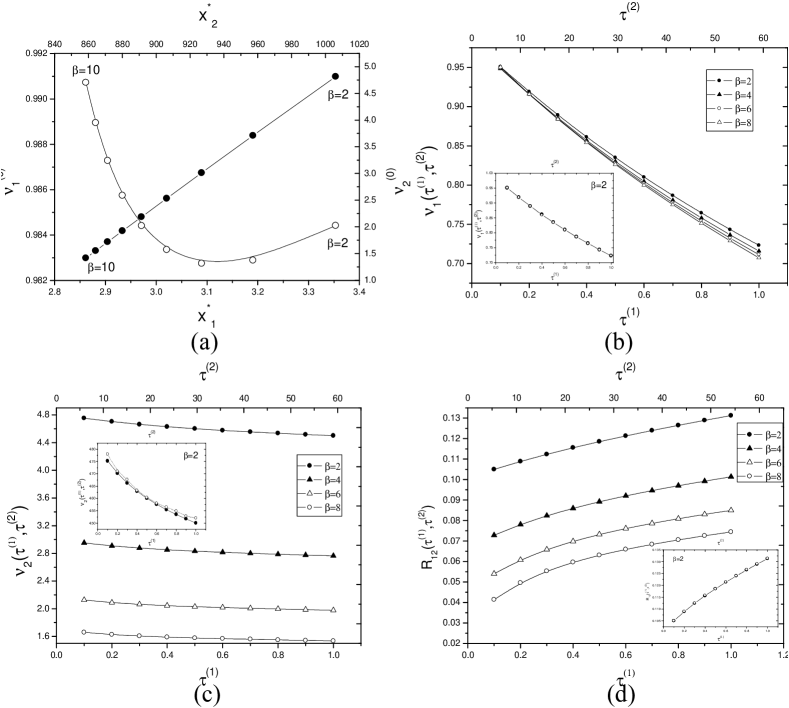
Figure 1: The fluctuations for autoregulatory networks:   For the case of white noise, the Fano factors, $\nu_{1}^{\left(0\right)}$ (hollow circles, left vertical) and $\nu_{2}^{\left(0\right)}$ (black dots, right vertical), versus the concentrations of mRNA (lower horizontal) and protein (upper horizontal) at the stable points for different Hill coefficients $\beta$ are shown in $\left(a\right)$. For the case of Gaussian colored noise, the Fano factors, $\nu_{1}\left(\tau^{\left(1\right)},\tau^{\left(2\right)}\right)$ and $\nu_{2}\left(\tau^{\left(1\right)},\tau^{\left(2\right)}\right)$, and the correlation coefficients of noises $R_{12}\left(\tau^{\left(1\right)},\tau^{\left(2\right)}\right)$ versus the correlation times of noises, $\tau^{\left(1\right)}$ (lower horizontal) and $\tau^{\left(2\right)}$ (upper horizontal), at the stable points for different Hill coefficients $\beta$ are shown in $\left(b\right)$, $\left(c\right)$, and $\left(d\right)$, respectively.

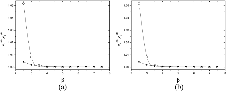
Figure 2: The Fano factors of toggle switch, $\nu_{1}^{\left(0\right)}$ (hollow circles) and $\nu_{2}^{\left(0\right)}$ (black dots), versus the Hill coefficient $\beta$ are shown in $\left(a\right)$ for the stable point $A$ and in $\left(b\right)$ for the stable point $B$. Note that while $\nu_{1}^{\left(0\right)}$ and $\nu_{2}^{\left(0\right)}$ are shown with the same vertical scale in $\left(a\right)$, the left vertical scale is for $\nu_{1}^{\left(0\right)}$ and the right vertical scale is for $\nu_{2}^{\left(0\right)}$ in $\left(b\right)$.

The two variables of auto-regulatory network, $x_{1}$ and $x_{2}$, are referred to the concentrations of mRNA and protein, respectively. For the functions $R_{i}\left(x\right)$ in the drift force of Eq. (6), we adopt the most common noise-attenuating regulatory mechanism, called negative feedback and described by Hill function,

$$R_{1}\left(x_{2}\right)=\frac{k_{\max}}{1+\left(x_{2}/k_{d}\right)^{\beta}},$$ (37)

to regulate the production of mRNA, and set

$$R_{2}\left(x_{1}\right)=k_{2}x_{1}.$$ (38)

Here $k_{\max}$ is the maximum transcription rate of mRNA, $k_{d}$ is the binding constant specifying the threshold protein concentration at which the transcription rate is half its maximum value, $\beta$ is the Hill coefficient, and $k_{2}$ is the translation rate of protein $k_{2}$. Then, a stable equilibrium, $x^{\ast}$, can be characterized by two conditions: $\ \theta^{\left(1\right)}\theta^{\left(2\right)}-r_{1}\left(x_{2}^{\ast}\right)k_{2}>0$ and $\theta^{\left(1\right)}+\theta^{\left(2\right)}>0$ with $r_{1}\left(x_{2}^{\ast}\right)=\left.\partial R_{1}\left(x_{2}\right)/\partial x_{2}\right|_{x_{2}=x_{2}^{\ast}}$. Subsequently, one can use Bendixson’s criterion to further conclude that there are no cycles and only one equilibrium exists bendixson .

We mainly follow Refs. thattai ; tao-c to specify the values of the parameters as follows. The half-lifetimes of mRNA molecules and proteins are set as $2$ minutes and $1$ hour, respectively; this leads to $\theta^{\left(1\right)}=\left(\ln 2\right)/2$ and $\theta^{\left(2\right)}=\left(\ln 2\right)/60$ in the unit of $\left(\min\right)^{-1}$. The average size of a burst of proteins, $b=k_{2}/\theta^{\left(1\right)}$, is set as $10$. This leads to $k_{2}=5\left(\ln 2\right)$. By using the fact that the protein concentration is about $1200$ when $\beta=0$ (no feedback), we set $k_{\max}=3$ remark . To study the effect of the strength of negative feedback on the fluctuation of the system, we vary the parameters $\beta$ from $2$ to $10$, while the $k_{d}$ value is fixed as $800$.

We first consider the case of white noise. Based on Eqs. (32)-(34), we obtain the $\nu_{1}^{\left(0\right)}$and $\nu_{2}^{\left(0\right)}$ values for $\beta$ ranging from $2$ to $10$, and the results are shown in Fig. 1(a). The characteristic features revealed from the results are summarized as follows. The $\nu_{2}^{\left(0\right)}$ value is much larger than the corresponding $\nu_{1}^{\left(0\right)}$ value, and it decreases as $\beta$ increases. This leads to the well-known conclusions that the stochastic fluctuations occur mainly at the translation level, and the negative feedback may enhance the stability of the system. On the other hand, the $\nu_{1}^{\left(0\right)}$ value decreases from $\nu_{1}^{\left(0\right)}=0.9844$ at $\beta=2$, reaches the minimum $\nu_{1}^{\left(0\right)}=0.9827$ at $\beta=4$, and then increases to $\nu_{1}^{\left(0\right)}=0.9907$ at $\beta=10$. All the $\nu_{1}^{\left(0\right)}$ values are very close to but always less than one. This implies that the process of transcription is sub-Poissonian. We then consider the effect of non-zero correlation time of noise on the fluctuation of the system based on Eqs. (28)-(30). First, we show the plots of $\nu_{1}\left(\tau^{\left(1\right)},\tau^{\left(2\right)}\right)$ and $\nu_{2}\left(\tau^{\left(1\right)},\tau^{\left(2\right)}\right)$ versus $\beta$ for $\left(\tau^{\left(1\right)},\tau^{\left(2\right)}\right)=\left(0.1,6\right)$, $\left(0.2,12\right)$, $\left(0.4,24\right)$, and $\left(0.6,36\right)$ in Figs. 1(b) and 1(c). Here the values of $\left(\tau^{\left(1\right)},\tau^{\left(2\right)}\right)$ are set as the multiples $10$, $20$, $40$, and $60$ of the half-lifetimes of mRNA and protein, respectively. The results indicate that the fluctuations are reduced by the amount proportional to the correlation time value of the noise. However, the reduction is less significant for protein owing to its long half-lifetime when compared with that of mRNA. Moreover, the effect of reduction, in general, is enhanced for a larger Hill coefficient, but this is not very significant for mRNA owing to the nature of the sub-Poissonian process. We also show the effect of the correlation time of noise on the correlation coefficient between $x_{1}$ and $x_{2}$ in Fig. 1(d), where the plots of $R_{12}\left(\tau^{\left(1\right)},\tau^{\left(2\right)}\right)$ versus $\beta$ for five sets of $\left(\tau^{\left(1\right)},\tau^{\left(2\right)}\right)$ values are displayed. The results indicate that the correlation coefficient $R_{12}$ increases with the correlation times of the noises but decreases with the Hill coefficient. Moreover, as the consequence of sub-Poissonian distribution for the mRNA component, the $R_{12}$ values between two components are very small, ranged between $0.0202$ and $0.1213$.

The analytical results given by Eqs. (28)-(30) are obtained with the approximation of linearization about a stable equlibrium. To test the validity of such an approximation, we solve the stochastic differential equations numerically by using Heun’s method. This numerical method is a stochastic version of the Euler method, which reduces to the second-order Runge-Kutta method in the absence of noise toral . The numerical simulations are in a very good agreement with the analytical results as shown in Figs. 1(b)-1(d) for $\beta=2.0$.

IV.2 Toggle switch

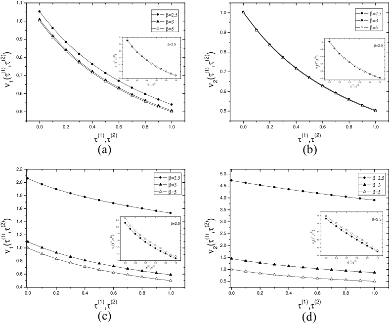
Figure 3: The fluctuations of toggle switch for the case of Gaussian colored noise: The Fano factors, $\nu_{1}\left(\tau^{\left(1\right)},\tau^{\left(2\right)}\right)$ and $\nu_{2}\left(\tau^{\left(1\right)},\tau^{\left(2\right)}\right)$, versus the correlation times of noises, $\tau^{\left(1\right)}$ and $\tau^{\left(2\right)}$ for different Hill coefficients $\beta$ are shown in $\left(a\right)$ and $\left(b\right)$ for the stable point $A$ and $\left(c\right)$ and $\left(d\right)$ for the stable point $B$. Note that $\tau^{\left(1\right)}$ is set to be equal to $\tau^{\left(2\right)}$ in the calculations of $\nu_{1}$ and $\nu_{2}$, and the values of $\nu_{1}$ and $\nu_{2}$ for $\tau^{\left(1\right)}=\tau^{\left(2\right)}=0$ are the results for the case of white noise.

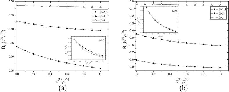
Figure 4: The correlation coefficients of noises of toggle switch, $R_{12}\left(\tau^{\left(1\right)},\tau^{\left(2\right)}\right)$, versus the correlation times of noises, $\tau^{\left(1\right)}$ and $\tau^{\left(2\right)}$ for different Hill coefficients $\beta$ are shown in $\left(a\right)$ for the stable point $A$ and in $\left(b\right)$ for the stable point $B$. Here $\tau^{\left(1\right)}$ is set to be equal to $\tau^{\left(2\right)}$, and the results for $\tau^{\left(1\right)}=\tau^{\left(2\right)}=0$ correspond to the case of white noise.

A toggle switch consists of two transcription factors with concentrations $x_{1}$ and $x_{2}$; the transcription factors can regulate each other’s synthesis through the negative feedback mechanism. Such genetic circuits often exhibit two stable states, referred as $A\left(x_{1}^{\ast},x_{2}^{\ast}\right)$ and $B\left(x_{1}^{\ast},x_{2}^{\ast}\right)$, for which, the $x_{1}$ component is dominant with almost vanishing $x_{2}$ component for the state $A$, and vice versa for the state $B$. The distinct two stable states can be switched either spontaneously or by a driven signal. A plasmid of this type in Escherichia coli has been engineered by Gardner, Cantor, and Collins gardner . For this, correspondingly, the degradation rates are rescaled to $\theta^{\left(1\right)}=\theta^{\left(2\right)}=1$; the regulation functions in the drift force of Eq. (6) then become

$$R_{1}\left(x_{2}\right)=\frac{\alpha_{1}}{1+x_{2}^{\beta}}$$ (39)

and

$$R_{2}\left(x_{1}\right)=\frac{\alpha_{2}}{1+x_{1}^{\gamma}}.$$ (40)

Here the parameter values are $\alpha_{1}=156.25$, $\alpha_{2}=15.6$, $\beta=2.5$, and $\gamma=1.0$. Such a specification leads to two stable states, $A\left(155.7634,0.0995\right)$ and $B\left(0.3324,11.7080\right)$.

The system with the regulation functions of Eqs. (39) and (40) exhibits the bistability over a wide rage of parameter values. In this study, we intend to analyze how the characteristics of the fluctuation change with the cooperative binding of the system. Thus, we calculate the variances and covariances along the parametric path increasing the Hill coefficient $\beta$ from $2.5$ to $7.5$ and keeping the other parameters to be the same as the previous values. As the $\beta$ value varied from $2.5$ to $7.5$, the loci of the two stable states are changed as follows. The $x_{1}^{\ast}$ value increases slightly from $155.7634$ up to $156.2500$ and the $x_{2}^{\ast}$ value decreases insignificantly from $0.0995$ down to $0.0992$ for the stable state $A$; meanwhile, the $x_{1}^{\ast}$ value decreases from $0.3324$ down to $1.759\cdot 10^{-7}$ and the $x_{2}^{\ast}$ value increases from $11.7080$ up to $15.6000$ for the stable state $B$. Accordingly, increasing the $\beta$ value will enhance the major component and suppress the minor component, and it will shift the location of the stable state $B$ more significantly than that of $A$.

We first consider the case of white noise for the study of fluctuations. The results of $\nu_{1}^{\left(0\right)}$and $\nu_{2}^{\left(0\right)}$ for different $\beta$ values are shown in Figs. 2(a) and 2(b) for the stable states $A$ and $B$, respectively. As indicated by the numerical results, the $\nu_{1}^{\left(0\right)}$and $\nu_{2}^{\left(0\right)}$ values all are larger than one; thus, the fluctuations are caused by super-Poissonian processes for both $A$ and $B$. This is opposite to the case of the auto-regulatory network, and it agrees with the results obtained by Tao tao . Moreover, the system in the stable state $B$ always possesses a larger deviation from Poissonian than that for $A$. But, the maximum deviation occurs at $\beta=2.5$ for both $A$ and $B$ at which, we have $\nu_{1}^{\left(0\right)}=1.0517$ and $\nu_{2}^{\left(0\right)}=1.0042$ for state $A$ and $\nu_{1}^{\left(0\right)}=2.0580$ and $\nu_{2}^{\left(0\right)}=4.7268$ for state $B$. Note that there is a big drop in the $\nu_{1}^{\left(0\right)}$and $\nu_{2}^{\left(0\right)}$ values for the system in the state $B$ when the $\beta$ value increases from $2.5$ to $3.0$. As the values of the finite correlation time of the noises set in, the resultant values of $\nu_{1}\left(\tau^{\left(1\right)},\tau^{\left(2\right)}\right)$ and $\nu_{2}\left(\tau^{\left(1\right)},\tau^{\left(2\right)}\right)$ for the values of $\tau^{\left(1\right)}=\tau^{\left(2\right)}$ ranging from $0$ to $1$ with $\beta=2.5$, $3$, and $6$ are shown in Figs. 3(a) and 3(b) for the states $A$ and in Figs. 3(c) and 3(d) for the state $B$. The results indicate a similar feature as that for the case of the auto-regulatory network, namely the fluctuations are reduced by the noises being correlated, and the longer is the correlation time, the bigger amount the fluctuation decreases. We also show the plots of $R_{12}\left(\tau^{\left(1\right)},\tau^{\left(2\right)}\right)$ versus $\tau^{\left(1\right)}\left(=\tau^{\left(2\right)}\right)$ for three different $\beta$ values in Figs. 4(a) and 4(b) for the stable states $A$ and $B$, respectively. All $R_{12}\left(\tau^{\left(1\right)},\tau^{\left(2\right)}\right)$ values shown in the figures are negative. This implies that the fluctuations of two components are anti-correlated, which reflects the fact that the two components are negatively regulated with each other. In particular, the system in the state $B$ with $\beta=2.5$ and $3.0$ is highly anti-correlated with $R_{12}^{\left(0\right)}=-0.8070$ and $-0.4453$, respectively. Also, the anti-correlation of fluctuations is enhanced as the finite correlation times of noises are set in.

The results shown in the above are also compared with those obtained from numerical simulations. The comparison is shown in the insets of Figs. 3(a)-3(d) and Figs. 4(a)-4(b) for $\beta=2.5$, and much larger differences in the Fano factors have been observed for the stable point $B$ than that for the stable point $A.$

V Summary

Noise due to stochastic fluctuations is always present and essential in the gene expression process due to low copy numbers of molecules and stochastic nature of biochemical reactions. A framework has been set up for the study of the noise by constructing the equivalent Langevin description of the system. By taking then the fluctuation as Gaussian colored noise, we first solve the Langevin equation, and then obtain the general formulae for the variances and covariance of a two-dimensional system near a stable equilibrium based on Ito calculus. For the latter, two important lemmas, concerning the variance of a Ito integral and the covariance between two Ito integrals, are established.

We apply the general formulae to the auto-regulation network and the toggle switch for the study of stochastic fluctuations of the systems, in particular, the effect caused by finite correlation time. In general, as correlation time of noise is set in, it will decrease the fluctuation and enhance the correlation of fluctuations. For the auto-regulation network, the fluctuations of mRNA concentration mirror a sub-Poissonian process with the Fano factor very close to but less than one. Consequently, this leads to the correlation coefficient between the fluctuations of mRNA and protein concentrations to be very small. For the toggle switch it is peculiar for one of the two stable states when the system has the Hill coefficient $\beta$ being around $2.5$; the fluctuations are caused by a process far away from Poissonian, and the fluctuations between two molecular components are highly anti-correlated. Aside from this, the fluctuations are caused by super-Poissonian processes with Fano factors very close to but larger than one for both concentrations in any of the two stable states; and this then leads to small but negative correlation coefficients between the fluctuations of two components. Moreover, as it has been shown, these analytical results are in a very good agreement with the numerical simulations.

To summarize, let us stress that it is more realistic to take into account the noise finite correlation time in order to study of stochastic fluctuations of gene regulatory networks. Meanwhile, in this work the noises of two components are still assumed to be independent, although the components couple with each other in the rate equations. It was shown cao that increasing the coupling strength between two noises may drive the system to transit from a bistable stationary probability distribution to a mono-stable one. Thus, it would be interesting to study the effect of coupled noises on the stochastic fluctuations in the gene regulatory networks. Besides, it will be also very interesting to extend the work to the case of a non-Gaussian colored noise bph .

We thank B.C. Bag, C.-K. Hu, and D. Salahub for discussions. The work of M.C.H., J.W.W., and Y.P.L. was partially supported by the National Science Council of Republic of China (Taiwan) under the Grant No. NSC 96-2112-M-033-006. K.G.P. was supported by Grants NSC 96-2811-M-001-018 and NSC 97-2811-M-001-055.

References

- (1) U. Alon, An Introduction to Systems Biology: Design Principles of Biological Circuits (CRC Press, 2006).
- (2) M. Ptashne, A Genetic Switch: Phage and Higher Organisms, 2nd ed. (Cell Press and Blackwell Scientific, Cambridge, MA, 1992).
- (3) J. Hasty, J. Pradines, M. Dolnik, and J.J. Collins, Proc. Natl. Acad. Sci. 97, 2075 (2000).
- (4) T.S. Gardner, C.R. Cantor, and J.J. Collins, Nature 403, 339 (2000).
- (5) M.B. Elowitz and S. Leibler, Nature 403, 335 (2000).
- (6) M.R. Atkinson, M.A. Savageau, J.T. Myers, and A.J. Ninfa, Cell 113, 597 (2003).
- (7) C.V. Rao, D.M. Wolf, and A.P. Arkin, Nature 420, 231 (2002).
- (8) J.M. Pedraza and J. Paulsson, Science 319, 339 (2008).
- (9) A. Becskei and L. Serrano, Nature 405, 590 (2000).
- (10) M. Thattai and A. van Oudenaarden, Proc. Natl. Acad. Sci. 98, 8614 (2001).
- (11) E.M. Ozbudak, M. Thattai, I. Kurtser, A.D. Grossman, and A. van Oudenaarden, Nature Genetics 31, 69 (2002).
- (12) J.L. Cherry and F.R. Adler, J. Theor. Biol. 203, 117 (2000).
- (13) P.B. Warren and P.R. ten Wolde, Phys. Rev. Lett. 92, 128101 (2004); J. Phys. Chem. B 109, 6812 (2005).
- (14) A. Lipshtat, A. Loinger, N.Q. Balaban, and O. Biham, Phys. Rev. Lett. 96, 188101 (2006); A. Loinger, A. Lipshtat, N.Q. Balaban, and O. Biham, Phys. Rev. E 75, 021904 (2007).
- (15) D.T. Gillespie, J. Chem. Phys. 81, 2340 (1977).
- (16) A. Arkin, J. Ross, and H.H. McAdams, Genetics 149, 1633 (1998).
- (17) N.G. van Kampen, Stochastic Processes in Physics and Chemistry (North-Holland, Amsterdam, 1992).
- (18) Y. Tao, J. Theor. Biol. 229, 147 (2004); 231, 563 (2004).
- (19) Y. Tao, Y. Jia, and T.G. Dewey, J. Chem. Phys. 122, 124108 (2005).
- (20) P. Jung and P. Hänggi, Phys. Rev. A 35, 4464 (1987); J. Opt. Soc. Am. B 5, 979 (1988).
- (21) V. Shahrezaei, J.F. Ollivier, and P.S. Swain, Molecular Systems Biology 4:196 (2008).
- (22) C.W. Gardiner, Handbook of Stochastic Methods, 3rd ed. (Springer-Verlag, Berlin, 2004).
- (23) G.E. Uhlenbeck and L.S. Ornstein, Phys. Rev. 36, 823 (1930); M.C. Wang and G.E. Uhlenbeck, Rev. Mod. Phys. 17, 323 (1945).
- (24) E. Coddington and N. Levinson, Theory of Ordinary Differential Equations (McGrow-Hill, N.Y., 1955).
- (25) The value was set as in Ref. thattai , this corresponds to a mean protein number when and leads to the increase of mean protein number as the Hill coefficient increases. Our setting, which is the same as that given in Ref. tao-c , leads to the decrease of mean protein number as increases. However, different settings do not change the picture obtained in this work.
- (26) R. Toral, in Computational Physics, Lecture Notes in Physics Vol. 448, edited by P. Garrido and J. Marro (Springer-Verlag, Berlin, 1995).
- (27) L. Cao, D.J. Wu, and S.Z. Ke, Phys. Rev. E 52, 3228 (1995).
- (28) B.C. Bag, K.G. Petrosyan, and C.-K. Hu, Phys. Rev. E 76, 056210 (2007).