Generating a Fractal Butterfly Floquet Spectrum in a Class of Driven SU(2) Systems: Eigenstate Statistics

Abstract

The Floquet spectra of a class of driven SU(2) systems have been shown to display butterfly patterns with multifractal properties. The implication of such critical spectral behavior for the Floquet eigenstate statistics is studied in this work. Following the methodologies for understanding the fractal behavior of energy eigenstates of time-independent systems on the Anderson transition point, we analyze the distribution profile, the mean value, and the variance of the logarithm of the inverse participation ratio of the Floquet eigenstates associated with multifractal Floquet spectra. The results show that the Floquet eigenstates also display fractal behavior, but with features markedly different from those in time-independent Anderson-transition models. This motivated us to propose a new type of random unitary matrix ensemble, called “power-law random banded unitary matrix” ensemble, to illuminate the Floquet eigenstate statistics of critical driven systems. The results based on the proposed random matrix model are consistent with those obtained from our dynamical examples with or without time-reversal symmetry.

I Introduction

The critical behavior of time-independent systems, especially in terms of the spectral statistics and the eigenstate statistics, has attracted great attention. On the spectrum side, Hofstadter’s butterfly spectrum of the Harper model has been a paradigm for critical spectral statistics, representing a multifractal spectrum harper ; hofstadter of a system exactly on the metal-insulator transition point. On the eigenstate side, mainly through studies in time-independent models, such as the power-law random banded matrix (PRBM) model PRBM and the standard Anderson tight-binding model (TBM) AndersonModel , it has been well-established that for a system on a metal-insulator transition point or the Anderson transition point AnderTrans01 , its eigenstates show clear fractal features. This background of understanding the critical behavior of time-independent systems motivated our interest in the critical behavior of periodically driven systems. Below we first introduce recent related studies of critical Floquet spectra, and then briefly describe the motivation and the results of this work.

It is well known that the Floquet (quasi-energy) spectrum of a delta-kicked version of the Harper model also displays Hofstadter’s butterfly patterns kicked_harper1 ; kicked_harper2 . Interestingly, though the kicked Harper model (KHM) can be classically chaotic, its spectrum, due to its fractal nature, does not follow the Bohigas-Giannoni-Schmit conjecture BGS at all. This makes the KHM not only a fruitful model for gaining new insights into the issue of quantum-classical correspondence in classically chaotic systems, but also an intriguing model to study critical spectral statistics. Indeed, for quite a long time, studies of fractal Floquet spectra were largely restricted to the KHM and its variants dana . In a proposal to experimentally realize Hofstadter’s butterfly Floquet spectrum in cold-atom laboratories, Wang and Gong JiaoJiangbin1 ; JMO recently demonstrated that Hofstadter’s butterfly Floquet spectrum can be synthesized by use of a double-kicked cold-atom rotor system DKRM under a quantum resonance condition. Lawton et al. JMP then showed that the butterfly Floquet spectrum of the cold-atom system studied in Refs. JiaoJiangbin1 ; JMO is equivalent to that of the standard KHM if and only if one system parameter takes irrational values. In addition to motivating a cold-atom realization of critical Floquet spectra of periodically driven systems, Refs. JiaoJiangbin1 ; JMO seem to have offered a general strategy for synthesizing critical Floquet spectra in driven systems.

Using an approach extended from Refs. JiaoJiangbin1 ; JMO , recently Wang and Gong JiaoJiangbin2 showed that the Floquet spectra of a class of driven SU(2) systems also display butterfly patterns and multifractal properties that are characteristics of highly critical spectra. This establishes a completely different class of critical driven systems without a connection with the KHM context. Interestingly, the driven SU(2) model in Ref. JiaoJiangbin2 can be understood as a simple extension of the well-known kicked top model (KTM) KTM in the quantum chaos literature. Because the KTM has just been experimentally realized in a cold ¹³³Cs system nature , it can be expected that a critical driven SU(2) system may also be experimentally realized using the collective spin of a ¹³³Cs atomic ensemble. An alternative experimental realization may be based on a driven two-mode Bose-Einstein condensate JiaoJiangbin2 ; 2modeBEC ; otherSU2 , which represents a strongly self-interacting driven system.

Given the above-mentioned class of driven quantum systems with critical Floquet spectra, it becomes necessary to study the behavior of the associated Floquet eigenstates. Theoretically speaking, because driven SU(2) systems always have a finite number of Floquet eigenstates, the eigenstate analysis becomes much easier than in the KHM, with the latter necessarily involving an infinite number of eigenstates for a fractal Floquet spectrum. A careful investigation of the Floquet eigenstates over the entire spectrum will help to better understand the critical behavior in time-dependent systems in general. Experimentally speaking, information about the eigenstate statistics may be more directly accessible to measurements than a fractal spectrum.

To analyze the critical behavior of the Floquet eigenstates in driven SU(2) systems, we adopt the same approach as in previous studies of time-independent systems. That is, we shall numerically examine the fluctuations of the eigenstates QPT . The eigenstate fluctuations can be characterized by a set of inverse participation ratios (IPR):

$$P_{q}^{(\lambda)}=\sum_{n}|\langle n|\phi_{\lambda}\rangle|^{2q},$$ (1)

where $\lambda$ is the index of the eigenstates, $|\phi_{\lambda}\rangle$ represents one eigenstate under investigation, and $\left\{|n\rangle\right\}$ are the basis states. For convenience we focus on the IPR $P_{2}$ (i.e., $q=2$). By analogy to critical eigenstate behavior in time-independent systems, we expect that $P_{2}$ scales anomalously with the Hilbert space dimension $N$ as

$$P_{2}^{(\lambda)}\sim N^{-D_{2}^{(\lambda)}},$$ (2)

where $D_{2}^{(\lambda)}$ is a fractal dimension of a particular eigenstate $|\phi_{\lambda}\rangle$. But is there also a unique fractal dimension $D_{2}$ for the average behavior of all the Floquet eigenstates, for example, via the slope of the averaged $\ln(P_{2})$, denoted $\langle\ln(P_{2})\rangle$, versus $\ln(N)$? To that end, we shall examine if, as the system gets closer to the thermodynamic limit ($N\rightarrow+\infty$), the distribution of $\ln(P_{2})$ shows signs of a scale-invariant form AnderTrans02 . In other words, whether the distribution function of $\ln(P_{2})$, denoted $\Pi[\ln(P_{2})]$, only shifts as $N$ varies.

Certainly, the system under our study has only a finite size $N$. In time-independent Anderson-transition studies using the PRBM or the TBM, it was conjectured that the variance of $\ln(P_{2})$, denoted $\sigma^{2}(N)$, scales with $N$ as

$$\sigma^{2}(N)=\sigma^{2}(\infty)-\frac{A}{N^{\gamma}},$$ (3)

with $\sigma^{2}(\infty)$, $A$, and $\gamma$ being three adjustable parameters cuevas01 . For a $d$-dimensional system on the Anderson transition point, it was shown that $\gamma$ is related to $D_{2}$ by

$$\gamma=\frac{D_{2}}{2\beta d},$$ (4)

where $\beta$ equals $1$ or $2$ depending upon whether or not the system has time-reversal symmetry cuevas02 . As one main task of this work, we shall examine if these results for time-independent systems still hold for critical Floquet eigenstates. Furthermore, we hope to see how the criticality of the eigenstates of unitary operators differs from the criticality of the eigenstates of self-adjoint operators. Results along this direction will also be relevant to recent investigations on the “unitary Anderson model” unit_Anderson , the Thue-Morse sequence generating multifractal eigenstates of the quantum baker’s map arul , the one-parameter model of quantum maps showing multifractal eigenstates Giraud , as well as recent experimental and theoretical studies of Anderson transition in kicked-rotor systems delande ; Jiao .

We now briefly summarize the main findings of this work. For the driven SU(2) systems studied here, we consider two different parameter regimes: in one regime the Floquet spectra display clear butterfly patterns, and in the other regime, the butterfly patterns of the Floquet spectra have dissolved due to increased strength of the driving fields. For both regimes, we find that $\Pi[\ln(P_{2})]$ is not as smooth as observed in the TBM or PRBM, indicating some non-universal features in dynamical systems. The $\Pi[\ln(P_{2})]$ for cases with dissolved butterfly patterns is however smoother. For either regime, it is found that the ensemble average $\langle\ln(P_{2})\rangle$ does scale linearly with $\ln(N)$, with the slope of the $\langle\ln(P_{2})\rangle$ vs $\ln(N)$ curve clearly defining the fractal dimension $D_{2}$ for all the eigenstates. We also find it possible to fit the variance of $\ln(P_{2})$ by Eq. (3), but with the exponent $\gamma$ given by

$$\gamma=\frac{D_{2}}{\beta d}$$ (5)

instead (with $d=1$); i.e., a factor of two is missing from the denominator as compared with Eq. (4) for time-independent critical systems. To further understand this difference, we propose a random matrix model, which we call “power-law random banded unitary matrix” (PRBUM) model. By tuning the parameters of the PRBUM, the $D_{2}$ value associated with the PRBUM can be varied. More interestingly, we observe that the variance $\sigma^{2}(N)$ of the PRBUM also follows Eq. (3), with the exponent $\gamma$ again given by Eq. (5). This suggests that our findings about the Floquet eigenstate statistics based on driven SU(2) systems do reflect some general aspects of critical Floquet eigenstates.

This paper is organized as follows. In Sec. II, we present detailed results of the eigenstates statistics in our driven SU(2) models, with or without time-reversal symmetry. In Sec. III, we introduce the PRBUM to represent a class of critical Floquet operators, discuss the statistics of the eigenstates of PRBUM, and then compare the associated results with those found in actual dynamical systems. In Sec. IV, we study the eigenstate statistics of the standard kicked top model KTM , which represents a classically chaotic, but non-critical, driven system. Section V concludes this work.

II Fractal statistics of the Floquet eigenstates in Driven SU(2) Models

The focus in Ref. JiaoJiangbin2 is on the fractal spectral statistics. Here, using the same model we study the statistics of the Floquet eigenstates. The first Floquet operator under study is given by

$$F=\exp\left(i\frac{\eta J_{z}^{2}}{2J}\right)\exp(-i\alpha J_{x})\exp\left(-i\frac{\eta J_{z}^{2}}{2J}\right)\exp(-i\alpha J_{x}),$$ (6)

where $J_{x},J_{y},J_{z}$ are angular momentum operators satisfying the SU(2) algebra and $J$ is the conserved total angular momentum quantum number that defines a $(2J+1)$-dimensional Hilbert space. Readers can refer to Ref. JiaoJiangbin2 for detailed descriptions and motivations of this model. This model is also called as a “double-kicked top model” (DKTM) in Ref. JiaoJiangbin2 .

Eigenstates of the $J_{z}$ operator are denoted as $|m\rangle$, with $J_{z}|m\rangle=m|m\rangle$. States $\{|m\rangle\}$ will be chosen as our representation for eigenstate analysis. To analyze the Floquet eigenstates, it is necessary to express the Floquet operator in symmetric basis states, a procedure that block-diagonalizes the Floquet matrix. On the one hand, this will simplify our analysis; on the other hand, this is necessary for the sake of comparison between an actual dynamical system and the PRBUM model proposed below.

The DKTM Floquet operator $F$ in Eq. (6) has a parity unitary symmetry $R^{\dagger}FR=F$ where $R=\exp(-i\pi J_{x})$. This symmetry can be used to block diagonalize the $F$ matrix into two disconnected sub-matrices associated with either odd-parity or even-parity subspaces. Without loss of generality we only present below results for the $J$-dimensional odd-parity subspace. Besides the parity symmetry, $F$ also has a time-reversal anti-unitary symmetry $TFT=F^{\dagger}$, with

$$T=\exp(i\alpha J_{x})K,$$ (7)

where $K$ is the complex conjugation operator. To explore the implication of this time-reversal symmetry for the eigenstate statistics, we shall also consider a variant of $F$, i.e.,

$$F^{\prime}=\exp\left(i\frac{\eta J_{z}^{2}}{2J}\right)\exp(-i\alpha J_{x})\exp\left(-i\frac{\eta J_{z}^{2}}{2J}\right)\exp(-i\alpha J_{y}).$$ (8)

Evidently, $F^{\prime}$ differs from $F$ only in the last factor, i.e., $\exp(-i\alpha J_{x})$ in $F$ is replaced by $\exp(-i\alpha J_{y})$. Because of this difference, we call $F$ in Eq. (6) the $J_{x}-J_{x}$ model and call $F^{\prime}$ the $J_{x}-J_{y}$ model. It is easy to check that the latter does not have the parity symmetry or the time-reversal symmetry. For the $J_{x}-J_{y}$ model, which cannot be reduced to any block-diagonal form, we examine the eigenstates of the full Floquet matrix.

For both cases we define a dimensionless system parameter,

$$\hbar_{\eta}\equiv\frac{\eta}{J}=\frac{1}{2}(\sqrt{5}-1)\pi.$$ (9)

This choice of $\hbar_{\eta}$ being $\pi$ times the golden mean is to ensure that the resulting Floquet eigenstate statistics is indeed representative of driven systems with fractal Floquet spectra. As detailed below, we consider two different regimes for the product $\alpha J$. In the first regime defined by $0.95\leq\alpha J\leq 1.05$, the Floquet spectra show clear butterfly patterns; in the second regime defined by $9.95\leq\alpha J\leq 10.05$, the butterfly spectra have dissolved, with fractal dimensions of the spectra increased JiaoJiangbin2 .

II.1 $J_{x}-J_{x}$ model

This is a time-reversal symmetric system. Because Dyson’s circular ensemble of random unitary matrices KTM with time-reversal symmetry is called “circular-orthogonal-ensemble” (COE), we regard the $J_{x}-J_{x}$ model as an example of critical COE statistics.

II.1.1 $0.95\leq\alpha J\leq 1.05$

Figure 1(a) shows the distributions of the logarithm of the IPR $P_{2}$, denoted $\Pi[\ln(P_{2})]$, for different $J$. It is seen that the distribution function $\Pi[\ln(P_{2})]$ is not as smooth as that observed in early Anderson-transition studies AnderTrans02 ; cuevas01 ; cuevas02 . Nevertheless, it is clear that as $J$ increases, the left tail of $\Pi[\ln(P_{2})]$ systematically shifts to the left direction associated with more negative $\ln(P_{2})$. The profile of $\Pi[\ln(P_{2})]$, though somewhat changes as $J$ increases, does maintain its main features as $J$ increases. Due to these features that are similar to early findings for the critical eigenstates in time-independent systems, it can be expected that the average of $\ln(P_{2})$ will show a scaling behavior with $\ln(J)$. As shown in Fig. 1(b), this is indeed the case. Therein, $\langle\ln(P_{2})\rangle$, obtained by averaging $\ln(P_{2})$ over all eigenstates (in the odd-parity subspace), displays an excellent linear behavior with $\ln(J)$. From the slope of the fitting line in Fig. 1(b), we are able to obtain the fractal dimension $D_{2}\simeq 0.274$.

The distribution profile $\Pi[\ln(P_{2})]$ in Fig. 1(a) is seen to display rich features, with significant fluctuations and multiple notable peaks. Qualitatively, this reflects that our system is an actual dynamical system and hence the underlying rich dynamics will manifest itself through some non-universal statistical features. Related to this observation we also note that in our calculations, all the Floquet eigenstates are treated equally and all of them are used for averaging. This is in contrast to the common procedure in analyzing time-independent critical systems, where only those energy eigenstates in a certain small energy window around zero eigenvalue are included to examine the distribution of $\ln(P_{2})$ AnderTrans02 ; cuevas01 ; cuevas02 . The justification for including all Floquet states in our analysis is as follows: the quasi-energy spectra lie on a unit circle and hence all states with different eigenphases on the unit circle should be treated on equal footing. To double check this understanding, we have also taken windows of different widths centered around zero value of the eigenphase and then calculate the distribution of $\ln(P_{2})$. No improvement in the smoothness of $\Pi(\ln P_{2})$ is found. Rather, we obtained similar distribution of $\ln(P_{2})$ with clear fluctuations. It is also tempting to connect the non-universal features of $\Pi(\ln P_{2})$ with the phase space structures of the underlying classical limit. However, such a perspective, which calls for a good understanding of quantum-classical correspondence in critical systems, is unlikely to succeed because the classical limit of our dynamical model is completely chaotic JiaoJiangbin2 .

In Fig. 1(c), we plot $\ln[\sigma^{2}(\infty)-\sigma^{2}(J)]$ vs $\ln(J)$ (filled circles), where $\sigma^{2}(J)$ is the variance of $\ln(P_{2})$ and $\sigma^{2}(\infty)$ is a fitting parameter, whose value is found by fitting our data points with the empirical formula given in Eq. (3). As seen in Fig. 1(c), the fitting is reasonably good, yielding that $[\sigma^{2}(\infty)-\sigma^{2}(J)]$ scales as $J^{-\gamma}$, with $\gamma=D_{2}$ [$D_{2}$ is already determined by the fitting in Fig. 1(b)], $\sigma^{2}(\infty)\simeq 0.68$, and $A\simeq 1.40$. Despite obvious fluctuations around the fitting curve, the result in Fig. 1(c) suggests that the tool borrowed from traditional Anderson-transition studies for time-independent systems can be still useful here. Furthermore (probably more interestingly), the fitting in Fig. 1(c) also unexpectedly reveals a big difference from what can be expected from Eq. (4) with $d=1$ and $\beta=1$: here $\gamma=D_{2}$ instead of $D_{2}/2$. Therefore, an intriguing difference between time-independent critical systems and periodically driven critical systems is observed here.

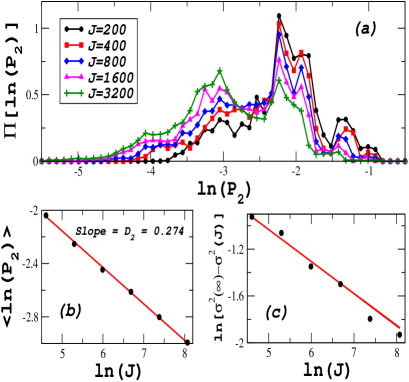
Figure 1: (Color online) (a) Distribution of $\ln(P_{2})$ for the $J_{x}-J_{x}$ model, with $J=200,400,800,1600$ and $3200,$ in the representation of odd-parity basis states defined in the text. The size of the Floquet matrix ensemble is important for numerical simulation. In order to construct the necessary ensemble, we consider a range of $\alpha$, i.e., $0.95\leq\alpha J\leq 1.05$, yielding respectively $4000,2000,1000,500$ and $250$ matrices for the different values $J$. (b) $\langle\ln(P_{2})\rangle$, the mean value of $\ln(P_{2})$ averaged over all Floquet eigenstates, as a function of $\ln(J)$. The slope of the fitting line gives $D_{2}\simeq 0.274$. (c) Logarithm of $[\sigma^{2}(\infty)-\sigma^{2}(J)]$ as a function of $\ln(J)$, where $J$ is the dimension of the odd-parity Hilbert subspace. Filled circles are our numerical results for the $J_{x}-J_{x}$ model, and the solid line is the fitting of the numerical results using the empirical formula given in Eq. (3) with $\sigma^{2}(\infty)=0.68$, $A=1.40$ and $\gamma=D_{2}$. The plotted variables here and in all other figures are dimensionless.

II.1.2 $9.95\leq\alpha J\leq 10.05$

As mentioned above, for this parameter regime the butterfly patterns in the Floquet spectra have dissolved almost completely. We present the associated eigenstate statistics in Fig. 2. In Fig. 2(a), we show the distribution profile of $\ln(P_{2})$ for different $J$. In contrast to the previous case shown in Fig. 1(a), $\Pi[\ln(P_{2})]$ is now much smoother (essentially only one peak is left). From the same panel, we also see a systematic left-shift of the distribution function as $J$ increases. This systematic left-shift leads to an evident linear behavior of the average value of $\ln(P_{2})$ as a function of $\ln(J)$, as shown in Fig. 2(b). The slope of the fitting line in Fig. 2(b) gives the fractal dimension $D_{2}\simeq 0.256$. Comparing this result with that in Fig. 1(b), one sees that though the fractal dimension of the Floquet spectra increases due to increasing $\alpha J$ JiaoJiangbin2 , the fractal dimension of the associated eigenstates may decrease.

In Fig. 2(c), we examine the variance of $\ln(P_{2})$ as a function of $\ln(J)$ (again, for the odd-parity subspace). Same as in Fig. 1(c), we fit our results with the empirical formula given in Eq. (3). The fitting in Fig. 2(c) is better than that in Fig. 1(c), consistent with the fact that the distribution of $\ln(P_{2})$ is quite smooth here. The fitting in Fig. 2(c) gives $\sigma^{2}(\infty)\simeq 0.77,A\simeq 1.59$, and $\gamma=D_{2}$, where the value of $D_{2}$ is found in Fig. 2(b). The finding that $\gamma$ is not equal to $D_{2}/2$ but $D_{2}$ again strengthens our early observation from Fig. 1.

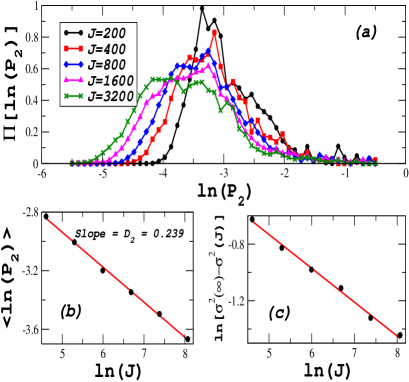
Figure 2: (Color online) (a) Distribution of $\ln(P_{2})$ for the $J_{x}-J_{x}$ model with $9.95\leq\alpha J\leq 10.05$ is presented for the odd-parity subspace. Other parameters are the same as in Fig. 1. (b) $\langle\ln(P_{2})\rangle$ is plotted as a function of $\ln(J)$. The slope of the fitting line gives $D_{2}\simeq 0.239$. (c) Logarithm of $[\sigma^{2}(\infty)-\sigma^{2}(J)]$ as a function of $\ln(J)$, where $J$ is the dimension of the odd-parity Hilbert subspace. Filled circles are our numerical results for the $J_{x}-J_{x}$ model, and the solid line is the fitting of the numerical results using the empirical formula given in Eq. (3), with $\sigma^{2}(\infty)\simeq 0.77$, $A=1.59$ and $\gamma=D_{2}$.

II.2 $J_{x}-J_{y}$ model

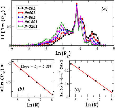
Figure 3: (Color online) (a) Distribution of $\ln(P_{2})$ for the $J_{x}-J_{y}$ model, with $J=100(4000),200(2000),400(1000),800(500),$ and $1600(250)$. The numbers in the brackets are the size of the Floquet matrix ensemble. The dimension of the Hilbert space is given by $N=2J+1$. (b) $\langle\ln(P_{2})\rangle$, the ensemble mean value of $\ln(P_{2})$ averaged over all Floquet eigenstates, as a function of $\ln(N)$. The slope of the curve of $\langle\ln(P_{2})\rangle$ vs $\ln(N)$ gives $D_{2}\simeq 0.259$. (c) Logarithm of $[\sigma^{2}(\infty)-\sigma^{2}(N)]$ vs $\ln(N)$. Filled circles are numerical results for the $J_{x}-J_{y}$ model, and the solid line is the fitting of the numerical results using the empirical formula given in Eq. (3), with $\sigma^{2}(\infty)=0.92$, $A=1.04$, and $\gamma=D_{2}/2$.

To verify if our findings above are general, we now turn to the $J_{x}-J_{y}$ model [Eq. (8)]. Due to the lack of time-reversal symmetry here, this case can be regarded as an example of critical “circular-unitary-ensemble” (CUE) statistics. All the eigenstates of the Floquet operator $F^{\prime}$ will be considered.

II.2.1 $0.95\leq\alpha J\leq 1.05$

For this regime where the butterfly patterns of the Floquet spectra can be clearly seen, Fig. 3(a) displays the distribution of $\ln(P_{2})$ for different Hilbert space dimension $N=2J+1$. Analogous to the previous case with time-reversal symmetry, $\Pi[\ln(P_{2})]$ displays interesting fluctuations. As $N$ increases, $\Pi[\ln(P_{2})]$ undergoes changes in its profile, shifts its left tail, but also maintains many features. In Fig. 3(b) we obtain again a nice linear scaling behavior of $\langle\ln(P_{2})\rangle$ with $\ln(N)$. From the slope of the linear scaling, we obtain the fractal dimension $D_{2}\simeq 0.259$. This $D_{2}$ value is different from that for the $J_{x}-J_{x}$ model with the same values of $\alpha J$(Note that the spectral statistics for the $J_{x}-J_{y}$ model also differs from that for the $J_{x}-J_{x}$ model JiaoJiangbin2 ).

Same as in Fig. 1(c), in Fig. 3(c) we study the variance of $\ln(P_{2})$ [now denoted $\sigma^{2}(N)$] as a function of $\ln(N)$, using the fitting formula given in Eq. (3). The fitting, though with clear fluctuations, yields that $[\sigma^{2}(\infty)-\sigma^{2}(N)]$ scales as $N^{-\gamma}$, with $\sigma^{2}(\infty)\simeq 0.92$, $A\simeq 1.04$, and $\gamma=D_{2}/2$ [$D_{2}$ value obtained from Fig. 3(b)]. Remarkably, though Eq. (4) with $d=1$ and $\beta=2$ (because of the lack of time-reversal symmetry) predicts $\gamma=D_{2}/4$, here we have $\gamma=D_{2}/2$ instead. The important common feature shared by the $J_{x}-J_{y}$ model and the $J_{x}-J_{x}$ model is thus the missing of a factor of 2 in the numerically obtained $\gamma$ value as compared with the empirical formula for time-independent critical systems. This interesting finding also supports the use of Eq. (3) as a tool for understanding Floquet eigenstate statistics. Our numerical observations here will be further strengthened by a random matrix model.

II.2.2 $9.95\leq\alpha J\leq 10.05$

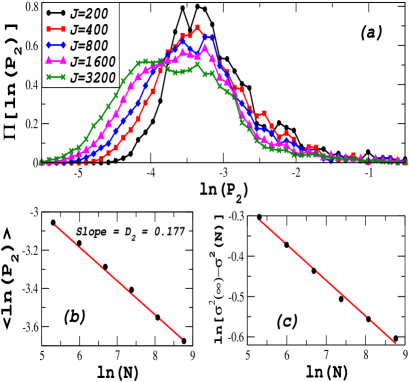
Figure 4: (Color online) (a) Distribution of $\ln(P_{2})$ for the $J_{x}-J_{y}$ model with $9.95\leq\alpha J\leq 10.05$ is presented for different Hilbert space dimension $N=2J+1$. Other parameters are the same as in Fig. 3. (b) $\langle\ln(P_{2})\rangle$ is plotted as a function of $\ln(N)$. The slope of this linear curve gives $D_{2}\simeq 0.177$. (c) Logarithm of $[\sigma^{2}(\infty)-\sigma^{2}(N)]$ vs $\ln(N)$. Filled circles are our numerical results for the $J_{x}-J_{y}$ model, and the solid line is the fitting of the numerical results using the empirical formula given in Eq. (3), with $\sigma^{2}(\infty)\simeq 1.11$, $A=1.17$ and $\gamma=D_{2}/2$.

Just like the $J_{x}-J_{x}$ model, in this regime the butterfly patterns of the Floquet spectra have dissolved. The statistical properties of the Floquet eigenstates are shown in Fig. 4. In Fig. 4(a), the distributions of $\ln(P_{2})$ is seen to be much smoother than those seen in Fig. 3(a). This is somewhat expected from our early findings in the $J_{x}-J_{x}$ model. Figure 4(b) shows a linear scaling of $\langle\ln(P_{2})\rangle$ vs $\ln(N)$, with its slope giving $D_{2}\simeq 0.177$. In Fig. 4(c), we study the variance of $\ln(P_{2})$ as a function of $\ln(N)$, as compared with the empirical formula given in Eq. (3): the fitting with the empirical formula is excellent, yielding $\sigma^{2}(\infty)\simeq 1.11,A\simeq 1.17$, and $\gamma=D_{2}/2$, where the value of $D_{2}$ is determined in Fig. 4(b). Once again, here we find $\gamma=D_{2}/2$ instead of $\gamma=D_{2}/4$ [as suggested by Eq. (4) with $\beta=2$].

III Eigenstate Statistics of PRBUM

In studies of time-independent critical systems, the PRBM model at criticality PRBM has proved to be fruitful. The PRBM is an ensemble of random Hermitian matrices whose matrix elements $\{H_{ij}\}$ are independently distributed Gaussian random numbers with mean $\langle H_{ij}\rangle=0$ and the variance satisfying

$$\sigma^{2}(H_{ij})=\left[1+\left(\frac{|i-j|}{b}\right)^{2g}\right]^{-1}.$$ (10)

The case $g=1$ represents the critical point and $0<b<\infty$ is a parameter characterizing the ensemble. A straightforward interpretation of this model is that it describes a one-dimensional sample with random long-range hopping, with the hopping amplitude decaying as $|i-j|^{-1}$. Motivated by our results above for critical Floquet states, we aim to propose a class of random unitary matrices, whose Floquet eigenstate statistics can show some general aspects of critical statistics and can be used to shed some light on actual dynamical systems. Our natural starting point for generating such random unitary matrices are the Hermitian PRBM.

III.1 Algorithm

To generate a random unitary matrix from a Hermitian matrix in the PRBM ensemble, we employ the algorithm by Mezzadri, whose original motivation is to generate CUE random matrices Mezzadri from general Gaussian random matrices. For the sake of completeness, we have presented a description of Mezzadri’s algorithm in Appendix A. For our purpose, that is, to generate a critical random unitary matrix, we first set the starting point of Mezzadri’s algorithm as a PRBM ensemble at the critical point ($g=1.0$). We then generate an ensemble of random unitary matrices (denoted $U$) of the CUE class. Significantly, because of the use of PRBM as the input for Mezzadri’s algorithm, we find that the variance of the matrix elements $\{U_{ij}\}$ thus obtained also satisfies a power-law, i.e.,

$$\sigma^{2}(U_{ij})=a_{0}\left[1+\left(\frac{|i-j|}{b_{0}}\right)^{2g_{0}}\right]^{-1}.$$ (11)

Here the parameter $a_{0}$ is a common prefactor of the matrix elements, which can be determined by the unitary condition. The parameters $g_{0}$ and $b_{0}$ in Eq. (11) depend on the parameters $g$ and $b$ of the PRBM used. As three computational examples, panels (d)-(f) of Fig. 5 present the dependence of $\ln[a_{0}/\sigma^{2}(U_{ij})-1]$ upon $\ln|i-j|$, for three ensembles of random unitary matrices we generated, with sizes $N=500,1000$, and $2000$. If the scaling of $\sigma^{2}(U_{ij})$ with $|i-j|$ is indeed a power law as described by Eq. (11), then one should see a linear dependence of $\ln[a_{0}/\sigma^{2}(U_{ij})-1]$ in $\ln|i-j|$. This is indeed the case in Figs. 5(d)-(f). Note that the deviations in Figs. 5(d)-(f) from the fitting straight lines at very large values of $\ln|i-j|$ are due to two trivial reasons. First, for very large $|i-j|$, the value of $\sigma^{2}(U_{ij})$ is vanishingly small and hence $\ln[1/\sigma^{2}(U_{ij})-1]$ becomes extremely large, thus yielding large fluctuations. Second and more importantly, for a fixed matrix size, if $|i-j|$ is very large, then the available number of matrix elements become insufficient for good statistics. Indeed, as the matrix size increases from $N=500$ to $N=2000$, it is seen from Figs. 5(d)-(f) that the validity window of the linear fitting gradually extends to larger values of $\ln|i-j|$.

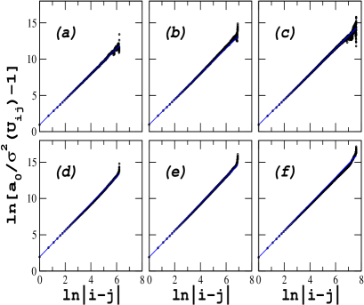
Figure 5: (Color online) The variance of the matrix elements of the random unitary matrices generated by Mazzadri’s algorithm with PRBM as the input. To demonstrate the power law scaling, the dependence of $\ln(a_{0}/\sigma^{2}(U_{ij})-1)$ on $\ln|i-j|$ is plotted, where $U_{ij}$ represents a matrix element at the $i$th row and $j$th column. Here the PRBM ensemble as the input is set at the critical point $g=1.0$ with the parameter $b=0.1$. Panels (a)-(c) are for PRBUM-COE, with the dimension $N=500,1000,$ and $2000$, respectively. The fitting function of Eq. (11) (solid lines) gives $a_{0}=0.165\pm 0.004$, $b_{0}=0.575\pm 0.003$, and $g_{0}=0.875\pm 0.002$. Panels (d)-(f) are for PRBUM-CUE, with the dimension $N=500,1000,$ and $2000$, respectively. The fitting function of Eq. (11) (solid lines) yields $a_{0}=0.277\pm 0.005$, $b_{0}=0.355\pm 0.004$, and $g_{0}=0.921\pm 0.001$.

The random unitary matrices generated in the above manner, with their matrix elements satisfying the power-law scaling of Eq. (11), are defined as “power-law random banded unitary matrix” of the CUE type (PRBUM-CUE). As detailed in Appendix A, one can then generate PRBUM of the COE type (PRBUM-COE) via $V=UU^{T}$. As shown in panels (a)-(c) of Fig. 5, the variance of the matrix elements of PRBUM-COE also obeys Eq. (11), with different values of $g_{0}$ and $b_{0}$.

To check whether the PRBUM-COE and PRBUM-CUE ensembles show critical statistics, we analyzed their eigenstates, especially in terms of the distribution and the scaling of $\ln(P_{2})$. It is found that as we tune the parameter $b$ of the PRBM used in the algorithm, the resulting fractal dimensions $D_{2}$ can be also tuned continuously. For example, the $D_{2}$ value of PRBUM can be made close to that of our driven SU(2) models. In particular, at $b=0.1$, we obtain $g_{0}\simeq 0.92$ for PRBUM-COE and $g_{0}\simeq 0.88$ for PRBUM-CUE, yielding $D_{2}\simeq 0.279$ and $D_{2}\simeq 0.251$, respectively. These two $D_{2}$ values are quite close to the $D_{2}$ values of the $J_{x}-J_{x}$ and $J_{x}-J_{y}$ models found in Fig. 1 and Fig. 3. Below we describe these findings in detail.

III.2 PRBUM-COE

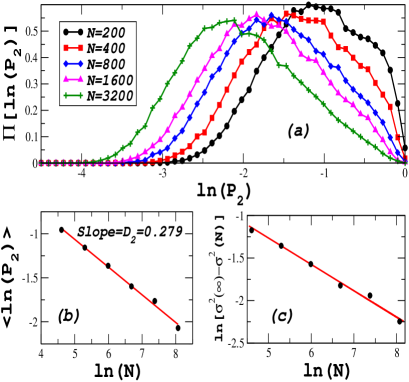
Figure 6: (Color online) (a) Distribution of $\ln(P_{2})$ obtained for PRBUM-COE, with the matrix dimension $N=200(4000),400(2000),800(1000),1600(500)$ and $3200(250)$. The numbers in the brackets give the size of the ensemble. (b) Same as in Fig. 1(b) and Fig. 2(b), yielding $D_{2}\simeq 0.279$. (c) Same as in Fig. 1(c) and Fig. 2(c), but with $J$ replaced by $N$. The fitting curve gives $\sigma^{2}(\infty)\simeq 0.60$, $A\simeq 1.33$, and $\gamma=D_{2}$.

This random unitary matrix ensemble is intended to model a critical Floquet operator with time-reversal symmetry. The results for PRBUM-COE generated from PRBM with $b=0.1$ are shown in Fig. 6. In Fig. 6(a), we show the distributions of $\ln(P_{2})$ for different values of the matrix dimension $N$ (which is the counterpart of $J$ in the $J_{x}-J_{x}$ model), with all the eigenstates of the PRBUM-COE ensemble considered. In contrast to the $J_{x}-J_{x}$ dynamical model with a small $\alpha J$ [see Fig. 1(a)], $\Pi[\ln(P_{2})]$ here displays very smooth behavior. Figure 6(b) depicts a nice linear relation between $\langle\ln P_{2}\rangle$ and $\ln(N)$. The slope of the straight line in Fig. 6(b) gives the fractal dimension $D_{2}\simeq 0.279$, a value close to that in the $J_{x}-J_{x}$ model with $0.95\leq\alpha J\leq 1.05$. As in Fig. 1(c), Fig. 6(c) shows the fitting of the variance of $\ln(P_{2})$ with $N$, using Eq. (3). Interestingly, the values of the fitting parameters are found to be $\sigma^{2}(\infty)\simeq 0.60$, $A=1.33$, both are similar to those determined in Fig. 1(c). More interestingly, this fitting shows that $[\sigma^{2}(\infty)-\sigma^{2}(N)]$ scales as $N^{-\gamma}$, with $\gamma=D_{2}$. This supports our finding in Fig. 1(c) and Fig. 2(c). We have also studied other cases of PRBUM-COE using other PRBM as the input of Mezzadri’s algorithm. For example, we find that if the parameter $b$ is set at $\sim 0.08$, then the $D_{2}$ of the PRBUM-COE ensemble is around 0.24, which is close to the $D_{2}$ value previously found in the $J_{x}-J_{x}$ model with $9.95\leq\alpha J\leq 10.05$. These results clearly support our use of PRBUM-COE to illuminate the critical eigenstate statistics in the $J_{x}-J_{x}$ model.

III.3 PRBUM-CUE

This ensemble aims to model a critical Floquet operator without time-reversal symmetry. All eigenstates of an ensemble of PRBUM-CUE matrices are used for our statistical analysis. For $b=0.1$, Fig. 7(a) displays $\Pi[\ln(P_{2})]$ versus $\ln(P_{2})$, showing again a smooth dependence. Figure 7(b) shows the corresponding $\langle\ln(P_{2})\rangle$ versus $\ln(N)$, which yields the fractal dimension $D_{2}\simeq 0.251$. In Fig. 7(c), we fit the dependence of $\ln[\sigma^{2}(\infty)-\sigma^{2}(N)]$ in $\ln(N)$, yielding $[\sigma^{2}(\infty)-\sigma^{2}(N)]\sim N^{-\gamma}$, with $\gamma=D_{2}/2$ [instead of $D_{2}/4$ predicted by Eq. (4)]. This also confirms our early observations in the $J_{x}-J_{y}$ model. The values of the fitting parameters are found to be $\sigma^{2}(\infty)\simeq 0.85$ and $A\simeq 1.05$, which are close to what we found in Fig. 3(c). We have also checked that if we perform analogous calculations for $b\sim 0.07$, then the $D_{2}$ value for the PRBUM-CUE ensemble will be close to that found in Fig. 4(b). Given these results, we are led to the conclusion that PRBUM as proposed above do share some general aspects with periodically driven systems having critical eigenstate statistics.

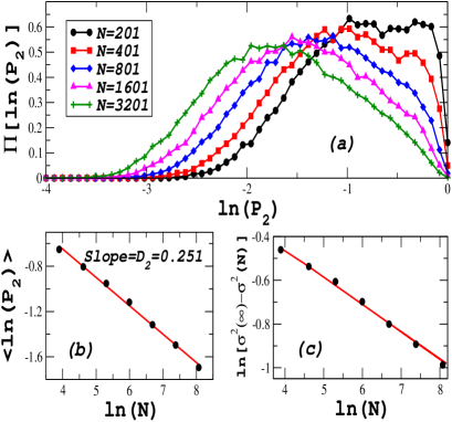
Figure 7: (Color online) (a) Distribution of $\ln(P_{2})$ obtained for PRBUM-CUE, with the matrix dimension $N=201(4000),401(2000),801(1000),1601(500)$ and $3201(250)$. The numbers in the brackets give the size of the ensemble. (b) Same as in Fig. 3(b) and Fig. 4(b), yielding $D_{2}\simeq 0.251$. (c) Same as in Fig. 3(c) and Fig. 4(c), the fitting gives $\sigma^{2}(\infty)\simeq 0.85$, $A\simeq 1.05$, and $\gamma=D_{2}/2$.

IV Floquet eigenstate statistics of the kicked top model

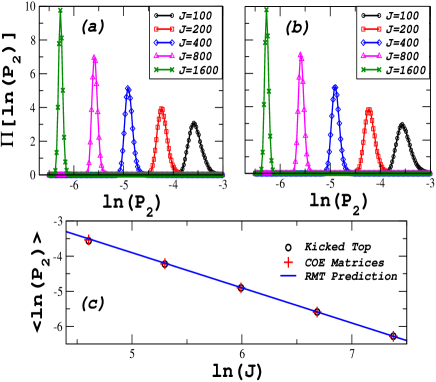
Figure 8: (Color online)(a) Distributions of $\ln(P_{2})$ for the standard classically chaotic kicked top model, for $J=100(4000),200(2000),400(1000),800(500)$ and $1600(250)$. The numbers in the brackets are the size of the Floquet matrix ensemble. In constructing the ensembles we have considered a range of $\alpha$, i.e., $0.95\leq\alpha\leq 1.05$. (b) Distributions of $\ln(P_{2})$ for the standard Dyson’s COE matrices, with the same matrix dimension as in the kicked top model and the same ensemble size. (c) Analogous to Fig. 1(b) and Fig. 7(b), the scaling behavior of $\langle\ln(P_{2})\rangle$ vs $\ln(J)$ is shown. Open circles are numerical results for the kicked-top model, crosses are numerical results associated with COE random matrices, and the solid curve represents the theoretical prediction from the random matrix theory. The scaling shows that $D_{2}=1$ in the standard kicked top model, which is dramatically different from our observations made from the double-kicked top model.

Finally, as a numerical “control” experiment, we study the Floquet eigenstate statistics of the standard kicked top model. This will help appreciate the difference between a normal driven system and a critical driven system, both of which can have a chaotic classical limit. Consider then the following Floquet operator for the standard kicked top model KTM ,

$$F_{\text{KTM}}=\exp\left(-i\frac{\eta J_{z}^{2}}{2J}\right)\exp(-i\alpha J_{x}),$$ (12)

which is just the last two factors of Eq. (6), with the same parity symmetry and time-reversal symmetry as the $J_{x}-J_{x}$ model. In addition, we set the parameter $\eta/J=\hbar_{\eta}$ at the same value as given in Eq. (9). We construct a statistical ensemble by considering a range of $\alpha$, i.e. $0.95\leq\alpha\leq 1.05$ (with chaotic classical limits). We carry out the Floquet eigenstate statistics in the odd-parity subspace, whose dimension is $J$. Because the classical limit is found to be chaotic, we compare the statistics with that associated with Dyson’s COE matrices in random matrix theory (RMT).

Figure 8(a) and (b) compare $\Pi[\ln(P_{2})]$ associated with $F_{\text{KTM}}$ with that obtained from COE matrices, for different $J$. The difference between the actual dynamical system and the COE can hardly be seen. Figure 8(c) depicts $\langle\ln(P_{2})\rangle$ as a function of $\ln(J)$, with the results of the kicked top (open circles) almost on top of those of COE matrices (crosses). The solid line in Fig. 8(c) represents the theoretical curve for $\langle\ln(P_{2})\rangle$ obtained from RMT, i.e., $\langle\ln(P_{2})\rangle\sim\ln 3-\ln(J)$. The agreement between numerical COE results, analytical RMT result, and the kicked top system as a classically chaotic dynamical system is almost perfect. From the curve shown in Fig. 8(c), it is clear that $D_{2}$ here is unity and as such the system does not show critical behavior. This non-critical behavior indicates that the Floquet states of the kicked top model are essentially random states, a feature fundamentally different from our double-kicked top system that has a butterfly spectrum and critical statistics in the Floquet eigenstates. It is also interesting to note that in Fig. 8(a) and (b), as $J$ increases, $\Pi[\ln(P_{2})]$ becomes narrower and develops higher peaks. This is an indication that, unlike the critical cases studied above, $\Pi(\ln P_{2})$ for the standard kicked top model approaches a Dirac-delta type singular function with zero width (i.e. $\sigma^{2}(\infty)\rightarrow 0$) as $J$ increases.

V Concluding Remarks

In this numerical study we have examined the statistics of the Floquet eigenstates of a recently proposed double-kicked top model with multifractal Floquet spectra. Following the methodologies used in studies of Anderson transition in time-independent systems, we have shown that the Floquet eigenstates associated with multifractal Floquet spectra also display critical behavior. In particular, we focus on the distribution of $\ln(P_{2})$ and examine how the quantity $\langle\ln(P_{2})\rangle$ averaged over all states scales with the dimension of the Hilbert space $N$. It is shown that $\langle\ln(P_{2})\rangle$ scales linearly with $\ln(N)$, with the slope of this linear scaling giving the fractal dimension $D_{2}$ of the Floquet eigenstates. The values of $D_{2}$ are found to be far from unity (as a comparison, we showed that similar analysis for a standard kicked top with a chaotic classical limit yields $D_{2}=1$), constituting strong evidence that the Floquet eigenstates are fractal and hence lying between localized and delocalized states. Though we have worked on $P_{2}$ only, we note that similar analysis can be done for $P_{q}$ defined in Eq. (1). One may then define a generalized fractal dimension $D_{q}$ and further establish the multifractal nature of the Floquet eigenstates.

The variance of $\ln(P_{2})$, denoted $\sigma^{2}(N)$ for a Hilbert space of dimension $N$, is also examined. In Anderson-transition studies with PRBM, $\sigma^{2}(N)$ is known to scale as $N^{-\gamma}$ with $\gamma=D_{2}/(2\beta)$ for one-dimensional systems, where $\beta=1\,(2)$ for a system with (without) time-reversal symmetry. By contrast, in our critical driven system, $\sigma^{2}(N)$ is seen to scale similarly, but with $\gamma=D_{2}/\beta$. This reflects an interesting difference between time-dependent systems and time-independent systems. Indeed, eigenstates of PRBM are to model those of critical Hermitian operators, whereas Floquet eigenstates of a critical driven system should be understood in terms of critical unitary operators. To justify this understanding, we have introduced a random unitary matrix ensemble called PRBUM, with the variance of the matrix elements of the unitary matrices following a power-law distribution. We show that the eigenstates of PRBUM share many critical statistical features with the double-kicked top model. Most important, the variance of $\ln(P_{2})$ of PRBUM does scale as $N^{-(D_{2}/\beta)}$, which is the same as in the double-kicked top model as a critical driven system. We hence anticipate that this scaling property of the variance of $\ln(P_{2})$ may be general in critical driven systems. These results complement the spectral results in Ref. JiaoJiangbin2 and should motivate further mathematical and theoretical studies in critical driven systems.

Appendix A Mezzadri’s algorithm

This is a simple and numerically stable algorithm to generate the CUE matrices from an ensemble of complex random matrices $\{Z_{i}\}$, whose elements are Gaussian distributed random numbers with mean zero and variance unity. In particular, applying the Gram-Schmmidt ortho-normalization method to the columns of an arbitrary complex matrix $Z_{i}$, one can factorize $Z_{i}$ as:

$$Z_{i}=Q_{i}R_{i},$$ (13)

where $Q_{i}$ is a unitary matrix and $R_{i}$ is an invertible upper-triangular matrix. One can easily prove that the above factorization is not unique. Because of this non-uniqueness, the random unitary matrices $\{Q_{i}\}$ are not distributed with Haar measure Mezzadri , i.e., the $\{Q_{i}\}$ matrices are not uniformly distributed over the space of random unitary matrices. Fortunately, this factorization can still be made unique by imposing a constraint on the $R_{i}$ matrices. By some group theoretical arguments, it was shown Mezzadri that if one finds a factorization such that the elements of main diagonal of $R_{i}$ become real and strictly positive, then $\{Q_{i}\}$ matrices would be distributed with Haar measure and hence form CUE. Following these results, the major steps of Mezzadri’s algorithm are the following. First, we start with an $N\times N$ complex Gaussian random matrix $Z_{i}$. Second, we factorize $Z_{i}$ by any standard $QR-$decomposition routine such that $Z_{i}=Q_{i}R_{i}$. Third, we create a diagonal matrix

$$\Lambda=\mbox{diag}\left(\frac{r_{11}}{|r_{11}|},\dots,\frac{r_{NN}}{|r_{NN}|}\right),$$

where $\{r_{ll}\}$ are the diagonal elements of $R_{i}$. As a final step, we define $R_{i}^{\prime}\equiv\Lambda^{-1}R_{i}$ and $Q_{i}^{\prime}\equiv Q_{i}\Lambda$. By construction, the diagonal elements of $R_{i}^{\prime}$ are always real and strictly positive, and as such $\{Q_{i}^{\prime}\}$ would be distributed with Haar measure and can be used to form the desired CUE. The symmetric COE matrices can be constructed from the CUE matrices in a very simple manner. In particular, let $U$ be a member of the CUE generated above, then it can be shown that $V=UU^{T}$ will be a member of COE. For the generation of PRBUM advocated in this work, we propose to replace $Z_{i}$ in the first step by a member in the PRBM ensemble that models Anderson transition. Though there is no mathematical theory for our procedure, the uniformly distributed eigenphases (not shown here) of our PRBUM ensemble thus generated suggest its uniform distribution.

References

- (1) P. G. Harper, Proc. Phys. Soc. London, Sect A 68, 874 (1955); 68, 879 (1955).
- (2) D. R. Hofstadter, Phys. Rev. B 14, 2239 (1976).
- (3) A. D. Mirlin et al, Phys. Rev. E 54, 3221 (1995).
- (4) P. W. Anderson, Phys. Rev. 109, 1492 (1958).
- (5) F. Evers and A. D. Mirlin, Rev. Mod. Phys. 80, 1355 (2008).
- (6) T. Geisel, R. Ketzmerick, and G. Petschel, Phys. Rev. Lett. 67, 3635 (1991).
- (7) See also some related papers: R. Lima and D. Shepelyansky, Phys. Rev. Lett. 67, 1377 (1991); R. Artuso et. al, ibid 69, 3302 (1992); R. Ketzmerick, K. Kruse, and T. Geisel, ibid 80, 137 (1998); I. I. Satija, Phys. Rev. E 66, 015202 (2002); J. B. Gong and P. Brumer, Phys. Rev. Lett. 97, 240602 (2006).
- (8) O. Bohigas, M. J. Giannoni, and C. Schmidt, Phys. Rev. Lett. 52, 1 (1984).
- (9) I. Dana and D. L. Dorofeev, Phys. Rev. E 72, 046205 (2005); I. Dana, Phys. Lett. A 197, 413 (1995); T. P. Billam and S. A. Gardiner, Phys. Rev. A80, 023414 (2009).
- (10) J. Wang and J. B. Gong, Phys. Rev. A 77, 031405(R) (2008).
- (11) J. Wang, A. S. Mouritzen, and J. B. Gong, J. Mod. Opt. 56, 722 (2009).
- (12) P. H. Jones et al., Phys. Rev. Lett. 93, 223002 (2004).
- (13) W. Lawton, A.S. Mouritzen, J. Wang, and J. B. Gong, J. Math. Phys. 50, 032103 (2009).
- (14) J. Wang and J. B. Gong, Phys. Rev. Lett. 102, 244102 (2009); Phys. Rev. E 81, 026204 (2010).
- (15) F. Haake, Quantum Signatures of Chaos 2nd Ed. (Springer-Verlag, Berlin, 1999).
- (16) S. Chaudhury, A. Smith, B. E. Andersdon, S. Ghose, and P. S. Jessen, Nature 461, 768 (2009).
- (17) Q. Zhang, P. Hänggi, and J. B. Gong, Phys. Rev. A77, 053607 (2008); New Journal of Physics, 10, 073008 (2008).
- (18) Q. Xie and W. Hai, Eur. Phys. J. D 33, 265 (2005); M.P. Strzys, E.M. Graefe, and H.J. Korsch, New J. Phys. 10, 013204 (2008); J. B. Gong, L. Molina-Morales, and P. Hänggi, Phys. Rev. Lett. 103, 133002 (2009).
- (19) S. Sachdev, Quantum Phase Transition (Cambridge, 2000).
- (20) Y. V. Fyodorov and A. D. Mirlin, Phys. Rev. B 51, 13403 (1995); F. Evers and A. D. Mirlin, Phys. Rev. Lett. 84, 3690 (2000); A. D. Merlin and F. Evers, Phys. Rev. B 62, 7920 (2000).
- (21) E. Cuevas et al., Phys. Rev. Lett. 88, 016401 (2002).
- (22) E. Cuevas, Phys. Rev. B 66, 233103 (2002).
- (23) E. Hamza, A. Joye, and G. Stolz, Lett. Math. Phys., 75, 255 (2006); Math. Phys. Anal. and Geom., 72, 381 (2009).
- (24) N. Meenakshisundaram and A. Lakshminarayan, Phys. Rev. E 71, 065303(R) (2005); A. Lakshminarayan and N. Meenakshisundaram, J. Phys. A 39, 11205 (2006).
- (25) J. Martin, O. Giraud, and B. Georgeot, Phys. Rev. E 77, 035201(R) (2008).
- (26) J. Chabé et al., Phys. Rev. Lett. 101, 255702 (2008); G. Lemarié et al., Phys. Rev. A 80, 043626 (2009).
- (27) J. Wang and A. M. García-García, Phys. Rev. E79, 036206 (2009); A. M. García-García and J. Wang, Phys. Rev. Lett. 94, 244102 (2005).
- (28) F. Mezzadri, Notices of the AMS 54, 592 (2007).