Modelling the evolution of planets in disks

Abstract

To explain important properties of extrasolar planetary systems (eg. close-in hot Jupiters, resonant planets) an evolutionary scenario which allows for radial migration of planets in disks is required. During their formation protoplanets undergo a phase in which they are embedded in the disk and interact gravitationally with it. This planet-disk interaction results in torques (through gravitational forces) acting on the planet that will change its angular momentum and result in a radial migration of the planet through the disk. To determine the outcome of this very important process for planet formation, dedicated high resolution numerical modeling is required. This contribution focusses on some important aspects of the numerical approach that we found essential for obtaining successful results. We specifically mention the treatment of Coriolis forces, Cartesian grids, and the FARGO method.

1 Introduction

After the discovery of now over 300 extrasolar planets (for an always up to date list, see: http://exoplanet.eu/ by Jean Schneider) the process of planet formation has now become again a major area of modern astrophysical research. The dynamical properties of the newly discovered planetary system show distinct differences with our own Solar System, see Udry et al. (2007) for a review. Most noticeable are very close in massive planets (hot Jupiters and Neptunes), high orbital eccentricities, and the occurrence of low order (2:1) mean-motion resonances. Some of these properties require an orbital evolution of the embedded planets through the disk. This migration process is very generic for young planets that are still embedded in the disk (Goldreich and Tremaine, 1980; Lin and Papaloizou, 1986b; Ward, 1997).

The formation of massive planets can take place primarily along two routes: (i) through gravitational instability of the protoplanetary disk (Boss, 1998). If the disk is sufficiently massive (about $0.1M_{*}$) spiral density arms will form which may turn gravitationally unstable resulting in local fragmentation and the formation of high density ’blobs’, i.e. the protoplanets. The main advantage of this scenario is its speed, as it is possible to form Jupiter sized planets within 100 orbital periods. A possible drawback is the requirement of relatively rapid cooling mechanisms in the disk, since the fragments can only collapse if they can cool sufficiently rapidly. Also, the existence of massive solid cores in the centers of the planets cannot easily be explained. (ii) through the core accretion process (Mizuno, 1980). In this second scenario the early growth of planets is accomplished by coagulation of small dust particles which are embedded in the gaseous protoplanetary disk. They collide, stick together and grow in mass until eventually (after several stages) a solid core of a few earth masses has be assembled. At this stage, gas accretion sets in and the planet can grow in mass up to several Jupiter masses.

Both models of planet formation must take place within a gaseous environment, i.e. the planet is still embedded within the surrounding protoplanetary accretion disk. In this case, the presence of the growing protoplanet in the disk will generate non-axisymmetric disturbances, the spiral arms (see Fig. 1). These pull gravitationally on the planet or, phrased differently, exert a torque ${\boldmath T}$ on the planet. As a consequence the angular momentum ${\boldmath L}$ of the planet will be changed $\dot{{\boldmath L}}={\boldmath T}$, and since for circular orbits ${\boldmath L}$ is only a function of the semi-major axis $a$ of the planet, the planet has to migrate. Hence, in both planet formation scenarios, the planet will move radially through the disk. Two observational facts are typically taken as indirect evidence that such a planetary migration process has indeed occurred. First, the existence of hot planets close to the star, as in-situ formation is difficult, and second the occurrence of mean motion resonances, as they require special locations of the planets which are very unlikely to occur just by chance.

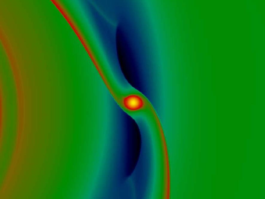
Figure 1: Density structure of an embedded Saturn mass planet in a protoplanetary disk. Clearly visible are the two spiral arms (red) and the lower density (gap, dark blue) at the orbit of the planet. (Courtesy: Aurélien Crida)

To calculate the evolution, i.e. the mass growth and migration of young planets in the disk, numerical simulations are typically employed. In this contribution we focus on the numerical aspect of planet-disk modeling, and will outline some of the necessary requirements to perform those simulations successfully.

2 Modelling

The majority of disk models assume a vertically thin disk which is approximated by an infinitesimally thin disk lying in the equatorial ($x-y$) plane. The motion of the gas is mostly described making a viscous hydrodynamic approach. Hence, the equations to be solved consist of the two-dimensional Navier-Stokes equations. Additionally the gravitational potentials of the central star and the embedded planets have to be added. The full equations including the viscous terms are given in Kley (1999). Initially, purely two-dimensional hydrodynamical simulations of this problem have been performed by several groups (Lin and Papaloizou, 1986a; Kley, 1999; Bryden et al., 1999; Lubow et al., 1999; Nelson et al., 2000; Masset, 2002; D’Angelo et al., 2002; Crida et al., 2006), subsequently extended to three-dimensions (Kley et al., 2001), and also with nested grids (D’Angelo et al., 2003). Later full 3D-MHD simulations with embedded planets have been added (Nelson and Papaloizou, 2003; Winters et al., 2003). All of these initial models used a locally isothermal equation of state simplifying the numerical modelling. Through fully 3D simulations including radiative effects, Paardekooper and Mellema (2006) demonstrated the crucial role the thermodynamics can play in determining the migration, an area that gains presently a lot of momentum (Paardekooper and Mellema, 2008; Baruteau and Masset, 2008; Kley and Crida, 2008). However, in this contribution we shall leave these most recent developments aside and focus in particular on some important numerical aspects of the planet-disk problem.

A standard setup for planet-disk modelers has been described recently within a European-wide code-comparison project where 22 Co-authors have used about 15 different codes on the same physical problem (de Val-Borro et al., 2006). In the comparison paper grid codes (upwind, Riemann), particle codes (SPH) and cylindrical or Cartesian grids are compared against each other. Anyone interested in performing planet-disk simulations is strongly encouraged to test and compare his/her results with that paper. One major simplification that is typically applied is the usage of an (locally) isothermal equations of state without any energy equation. For this case there exist also semi-analytical linear results for small mass planets (Goldreich and Tremaine, 1980; Ward, 1997). The principle outcome of such simulations is displayed in Fig. 1, which is based on a grid based simulation using a cylindrical coordinate system. An important quantity to plot is the radial profile of the azimuthally averaged surface density in the disk. This gives an indication of the accuracy of the angular momentum conservation and transport in the disk, which is particularly important to calculates reliable migration rate. Results obtained in the comparison project are displayed Fig. 2 for the density. While most of the codes agree, there are also important deviations. Let us concentrate on some important points in performing these simulations.

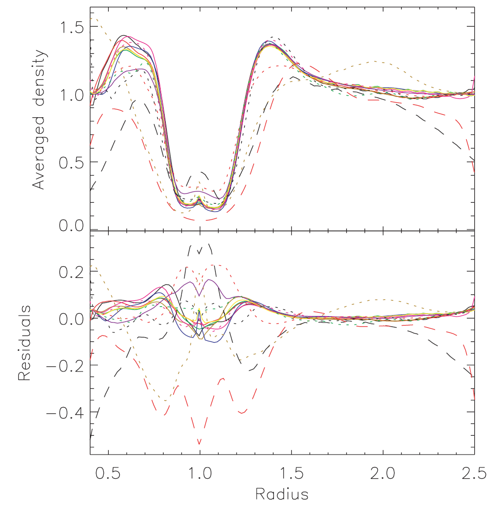
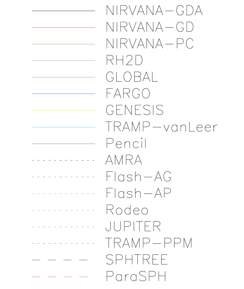
Figure 2: Azimuthally averaged density profile for an embedded Jupiter mass planet in a viscous ($\nu=10^{-5}$) and locally isothermal ($H/r=0.05$) disk after 100 orbital periods. Displayed are the results for different codes as given in the legend. Here the solid lines refer to upwind-codes (with the exception of the last, purple curve which refers to the high-order code PENCIL (Brandenburg and Dobler, 2002)), dotted lines to Riemann solver, and dashed lines to SPH codes. (Adapted from: de Val-Borro et al. (2006))

2.1 Coriolis terms

Often it is desirable to perform the simulations in a coordinate frame that corotates with the planet. In such a case additional source terms appear in the equations of motion. Taken at face value these additions imply non-conservation for the angular momentum. Through a reformulation of the $\varphi$ equation one can write an explicit conservation equation for the angular momentum (as viewed in the inertial frame). Only the usage of this conserving scheme yields the correct density distribution and reliable torques acting on the planet, as demonstrated by Kley (1998). A non-conservative scheme will typically require a much higher spatial resolution for obtaining equally good results.

Figure 3: 3D density distribution of the perturbed disk in the presence of an embedded planet calculated in the rotating frame. Left: explicit sources, non-conservation of angular momentum. Right: conservative formulation. (Adapted from: Kley (1998))

The difference of the two formulations is demonstrated in Fig. 3 where a Jupiter mass planet has been embedded in an accretion disk. The density distribution, in particular the slope near to the planet is very different in the two cases. The right panel refers to the conservative formulation and the obtained results are very close to the inertial case. The incorrect density gradient in the vicinity of the planet for the non-conservation case leads to wrong migration and mass accretion rates. Hence, when using a rotating reference frame, care should be taken to always write the angular momentum in conservative form.

2.2 The FARGO algorithm

Typically, the simulations as just described are performed in a cylindrical coordinate system ($r,\varphi$). In explicit codes the time step is limited by the Courant condition which states that in one time step the information can only be propagated over at most one gridcell to ensure numerical stability. In a highly supersonic accretion disk where the flow is basically on circles this yields

$$\Delta t<\frac{\Delta\varphi}{\omega}$$ (1)

where $\omega$ denotes the azimuthal angular velocity and $\Delta\varphi$ the azimuthal size of a gridcell. In a Keplerian disk $\omega$ scales as $\omega\propto r^{-3/2}$ and hence the timestep scales as $\Delta t\propto r^{3/2}$, i.e. the innermost rings with the smallest radii determine the size of the timestep, see also Fig. 4 left panel.

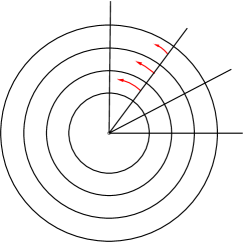
Figure 4: Left Illustration of the angular velocity in a Keplerian disk. The large inner velocities imply a very small timestep. Right The azimuthally averaged density for four kinds of simulations using the standard method and the FARGO-implementation (Masset, 2000a) both in an inertial and rotating reference frame.

In our case of planet disk-interaction the inner disk boundary must not be very close to the planet and, due to the Courant condition, this leads to very small timesteps. An excellent remedy of this problem has been suggested by (Masset, 2000a) who introduced the so-called FARGO-algorithm (Fast Advection in Rotating Gaseous Objects). This method relies on a directional splitting of the advection, where first the radial advection is performed in the standard way. The azimuthal part is then done in two parts: First an average angular velocity $\bar{\omega}_{i}$ is calculated for each ring $i$, and all quantities at each ring $i$ are shifted by an integer number of gridcells, $n_{i}$=Nint$(\bar{\omega}_{i}\Delta t/\Delta\varphi$), where Nint denotes the nearest integer function. This corresponds to a transport by the ’shift velocity’ ${\omega}_{i}^{SH}=n_{i}\Delta\varphi/\Delta t$. In the second step, all quantities are transported (in two sub-steps) with the remaining part of the angular velocity ${\omega}_{i}^{r}={\omega}_{i}-{\omega}_{i}^{SH}$ using the standard advection routine at hand. In this case the effective applied transport velocity (${\omega}_{i}^{r}$) in each ring is of the order of the deviations from the mean $\bar{\omega}_{i}$ which is much smaller than the Keplerian flow speed. Using this method, a large increase in the time-step can be achieved. Since the first shift-stip is exact, there is also a substantial reduction in diffusivity of the method. For details of the implementation see Masset (2000a, b). The code with all sources and improvements is available at the FARGO-webpage: http://fargo.in2p3.fr/. In Fig. 4 we demonstrate in the right panel the accuracy of the method by comparing 4 different integration methods. Calculated are runs for the inertial and rotating frame with either FARGO switched or not. Here, the disk extends radially from $[0.4;2.5]$ and the grid is covered by $128\times 384$ gridcells. This setup refers to the standard test case as described above (de Val-Borro et al., 2006). Displayed are the results after 25 orbits of the planet. Clearly all four cases yield very similar results. The runs were all done with a Courant number of $0.75$, and the used number of timesteps for the runs from top down have been: 51,000; 39,000; 5800; 5800. The first case (standard, inertial) needs the most timesteps, the second (standard, rotating) needs about 20% less due the the reduced angular velocities in the rotating frame. The last two FARGO-runs yield both (in the inertial and rotating frame) an identical number of timesteps, since the introduction of the shift brings all the rings essentially to the corotating frame. As seen in this case the speedup obtained with FARGO is about a factor of 9! In the general case the speedup depends on the radial range and the grid scaling. For a logarithmic radial grid an even larger speedup factor can be achieved. Obviously the FARGO-method gives the correct results and hence should definitely be the favored method when performing simulations of sheared flow in disks.

2.3 Coordinate System

As mentioned above, typical planet-disk simulations are performed using a cylindrical coordinate system, which is well adapted to the physics of the problem and yields automatically the important feature of angular momentum conservation. However, recently several simulations have been presented that utilize a Cartesian coordinate system on the planet-disk problem (Zhang et al., 2008; Pepliński et al., 2008; Lyra et al., 2008). This has inspired us to perform some test simulations in Cartesian coordinates as well, and evaluate the accuracy and requirements. For this purpose we used our standard code RH2D, which is a grid based code utilizing a 2nd order upwind scheme (monotonic transport), staggered grid and operator splitting Kley (1989). The code behaves quite similar to the well known ZEUS code. What we found first is that in the standard formulation, where advection is operator-split from the force terms, disk calculations (even without embedded planet) in Cartesian coordinates were not possible. We believe that this failure is due to the usage of operator splitting with the separation of advection and forces. Here, the disk structure is given by the equilibrium of gravity and inertial terms which are both large, have to cancel out, but are not done in one step.

A reformulation of the numerical scheme using a 2nd order TVD Runge-Kutta time-integrator (Shu and Osher, 1988) and no operator-splitting but otherwise identical method (staggered, monotonic transport) gave consisted results on disk evolution calculations.

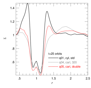
Figure 5: The azimuthally averaged density for different simulations using a Cartesian grid structure at two different resolutions (grey dotted line: $320\times 320$, red dashed line: $640\times 640$) or a cylindrical grid (black solid: $128\times 384$). The simulations refers to the same physical setup as above in Fig. 2.

The results for the standard problem after 25 orbits are displayed in Fig. 5 for two Cartesian runs with $320\times 320$ and $640\times 640$ gridcells in a square with length $[-2.5,2.5]$ in the $x$ and $y$ direction. As boundary conditions for these Cartesian runs we used the same damping conditions as in de Val-Borro et al. (2006). The smaller grid $320\times 320$ yields in the vicinity of the planet the same resolution as an $128\times 384$ grid in cylindrical coordinates, which is also displayed in Fig. 5. While the depth of the gap created by the planet is similar in all cases, its width varies considerably. The Cartesian runs do not seem to have converged even in the high resolution case. In the EU-comparison project, there have been two codes that used a Cartesian grid: The PENCIL code (purple line in Fig. 2) and the FLASH code (brown dashed line, labeled ‘Flash-AP’). Of these two, only the PENCIL code gave satisfactory results, where the gap width shows good agreement, but the gap is a little to shallow. On the other hand, the gap width is much larger for the FLASH code using a Cartesian coordinate system. Only the two SPH-codes (long dashed lines) show worse results in this test case. For the SPH-method, there seems to be a possible remedy which is currently tested (R. Speith, private communication). From these Cartesian simulations we conclude that i) due to the non-conservation and enhanced diffusion of angular momentum, a much higher resolution than in cylindrical codes is required for similar results, or ii) very high order schemes such as PENCIL have to be applied.

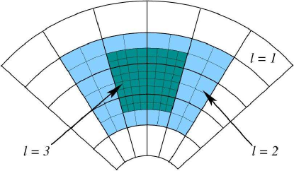
Figure 6: The grid structure of a nested grid with 2 levels of refinements. Around the fixed location of the planet (here assumed to be in the very center of the grids) the base grid ($l=1$) is covered by superimposed finer grids ($l=2,3$) to locally enhance the resolution. These grids are already in place from the very beginning of the simulations and not added later. (Adapted from: D’Angelo et al. (2002))

2.4 Nested Grids

Another important numerical issue refers to the fact that for an accurate calculation of the torques acting on the planet, the local as well as global structure of the disk is required simultaneously. To obtain this with one single grid would require a very large resolution indeed. A way out is to refine the grid structure in the vicinity of the planet. This has been attempted through the usage of a non-uniform spacing of the grid (Bate et al., 2003), which comes with the disadvantage of a large deformation of the gridcells near the planet. Another option is the usage of Nested Grids which has been utilized by D’Angelo et al. (2002). In such a case the base grid is refined locally at locations that are predefined (fixed) from the very beginning of the simulations, in contrast to adaptive mesh refinement (AMR) simulations. In the planet-disk interaction, frequently a non-moving (fixed) planet is assumed to simplify the equations and focus directly on the torque calculations. Here, the Nested Grid method is particularly well suited, as the planet can be placed naturally in the center of the whole grid-system, see Fig. 6, for the whole time evolution. The Nested Grid technique has been used first in 2D (D’Angelo et al., 2002) and later fully 3D simulations of embedded planets in disks (D’Angelo et al., 2003), where up to 7 sub-grids have been used which has allowed for the most detailed resolution of the Roche lobe of the protoplanet so far. Migration and mass accretion rates have been determined through these simulations and it has been found that non-linear effects begin to set in already at very small planetary masses, which has been confirmed later by Masset et al. (2006). To follow the planetary migration in a globally evolving disk with a large radial range, an interesting method has been suggested recently by Crida and Morbidelli (2007) who sandwich the active 2D region with one-dimensional (only radial grids) added at the inner and outer radius.

2.5 Summary

In this contribution we have discussed several important numerical issues related to planet-disk simulations. We have shown that, due to the physical symmetry of the problem, the usage of a cylindrical coordinate system is generally advantageous over a Cartesian one. In case of a rotating coordinate system the equations need to be reformulated to ensure angular momentum conservation. We have shown that a computational reformulation of the angular advection using the FARGO method leads to a substantial increase in the allowed size of the time-step. We have demonstrated the accuracy and achievable speed-up of the FARGO method by comparing the results to standard cases. Finally, we have shown that an increase in resolution near to the planet can been achieved through the usage of nested grids. Future numerical models of the planet-disk problem will involve three-dimensional analyzes which will include more physical effects such as self-gravity, radiation transport and magnetic fields.

2.6 Acknowledgements

This work has been sponsered in parts by the DFG grants KL-650/6, KL-650/7 and the Forschergruppe The Formation of Planets. The critical first growth phase through grant KL-650/11.

References

- Baruteau and Masset (2008) Baruteau, C. and Masset, F.: 2008, ApJ 672, 1054
- Bate et al. (2003) Bate, M. R., Lubow, S. H., Ogilvie, G. I., and Miller, K. A.: 2003, MNRAS 341, 213
- Boss (1998) Boss, A. P.: 1998, ApJ 503, 923
- Brandenburg and Dobler (2002) Brandenburg, A. and Dobler, W.: 2002, Computer Physics Communications 147, 471
- Bryden et al. (1999) Bryden, G., Chen, X., Lin, D. N. C., Nelson, R. P., and Papaloizou, J. C. B.: 1999, ApJ 514, 344
- Crida and Morbidelli (2007) Crida, A. and Morbidelli, A.: 2007, MNRAS 377, 1324
- Crida et al. (2006) Crida, A., Morbidelli, A., and Masset, F.: 2006, Icarus 181, 587
- D’Angelo et al. (2002) D’Angelo, G., Henning, T., and Kley, W.: 2002, A&A 385, 647
- D’Angelo et al. (2003) D’Angelo, G., Kley, W., and Henning, T.: 2003, ApJ 586, 540
- de Val-Borro et al. (2006) de Val-Borro, M., Edgar, R. G., Artymowicz, P., Ciecielag, P., Cresswell, P., D’Angelo, G., Delgado-Donate, E. J., Dirksen, G., Fromang, S., Gawryszczak, A., Klahr, H., Kley, W., Lyra, W., Masset, F., Mellema, G., Nelson, R. P., Paardekooper, S.-J., Peplinski, A., Pierens, A., Plewa, T., Rice, K., Schäfer, C., and Speith, R.: 2006, MNRAS 370, 529
- Goldreich and Tremaine (1980) Goldreich, P. and Tremaine, S.: 1980, ApJ 241, 425
- Kley (1989) Kley, W.: 1989, A&A 208, 98
- Kley (1998) Kley, W.: 1998, A&A 338, L37
- Kley (1999) Kley, W.: 1999, MNRAS 303, 696
- Kley and Crida (2008) Kley, W. and Crida, A.: 2008, A&A 487, L9
- Kley et al. (2001) Kley, W., D’Angelo, G., and Henning, T.: 2001, ApJ 547, 457
- Lin and Papaloizou (1986a) Lin, D. N. C. and Papaloizou, J.: 1986a, ApJ 307, 395
- Lin and Papaloizou (1986b) Lin, D. N. C. and Papaloizou, J. C. B.: 1986b, ApJ 309, 846
- Lubow et al. (1999) Lubow, S. H., Seibert, M., and Artymowicz, P.: 1999, ApJ 526, 1001
- Lyra et al. (2008) Lyra, W., Johansen, A., Klahr, H., and Piskunov, N.: 2008, ArXiv e-prints
- Masset (2000a) Masset, F.: 2000a, A&AS 141, 165
- Masset (2000b) Masset, F. S.: 2000b, in G. Garzón, C. Eiroa, D. de Winter, and T. J. Mahoney (eds.), Disks, Planetesimals, and Planets, Vol. 219 of Astronomical Society of the Pacific Conference Series, pp 75–+
- Masset (2002) Masset, F. S.: 2002, A&A 387, 605
- Masset et al. (2006) Masset, F. S., D’Angelo, G., and Kley, W.: 2006, ApJ 652, 730
- Mizuno (1980) Mizuno, H.: 1980, Progress of Theoretical Physics 64, 544
- Nelson and Papaloizou (2003) Nelson, R. P. and Papaloizou, J. C. B.: 2003, MNRAS 339, 993
- Nelson et al. (2000) Nelson, R. P., Papaloizou, J. C. B., Masset, F. S., and Kley, W.: 2000, MNRAS 318, 18
- Paardekooper and Mellema (2006) Paardekooper, S.-J. and Mellema, G.: 2006, A&A 459, L17
- Paardekooper and Mellema (2008) Paardekooper, S.-J. and Mellema, G.: 2008, A&A 478, 245
- Pepliński et al. (2008) Pepliński, A., Artymowicz, P., and Mellema, G.: 2008, MNRAS 386, 164
- Shu and Osher (1988) Shu, C.-W. and Osher, S.: 1988, Journal of Computational Physics 77, 439
- Udry et al. (2007) Udry, S., Fischer, D., and Queloz, D.: 2007, in B. Reipurth, D. Jewitt, and K. Keil (eds.), Protostars and Planets V, pp 685–699
- Ward (1997) Ward, W. R.: 1997, Icarus 126, 261
- Winters et al. (2003) Winters, W. F., Balbus, S. A., and Hawley, J. F.: 2003, ApJ 589, 543
- Zhang et al. (2008) Zhang, H., Yuan, C., Lin, D. N. C., and Yen, D. C. C.: 2008, ApJ 676, 639