On the effective permittivity of finite inhomogeneous objects

Abstract

A generalization of the S-parameter retrieval method for finite three-dimensional inhomogeneous objects under arbitrary illumination and observation conditions is presented. The effective permittivity of such objects may be rigorously defined as a solution of a nonlinear inverse scattering problem. In this respect the problems of S-parameter retrieval, effective medium theory, and even the derivation of the macroscopic electrodynamics itself, turn out to be all mathematically equivalent. We confirm analytically and observe numerically effects that were previously reported in the one-dimensional strongly inhomogeneous slabs: the non-uniqueness of the effective permittivity and its dependence on the illumination and observation conditions, and the geometry of the object. Moreover, we show that, although the S-parameter retrieval of the effective permittivity is scale-free at the level of problem statement, the exact solution of this problem either does not exist or is not unique. Using the results from the spectral analysis we describe the set of values of the effective permittivity for which the scattering problem is ill-posed. Unfortunately, real nonpositive values, important for negative refraction and invisibility, belong to this set. We illustrate our conclusions using a numerical reduced-order inverse scattering algorithm specifically designed for the effective permittivity problem.

I Introduction

The notion of an effective permittivity (conductivity, permeability) has been introduced within the effective-medium theory and was meant as a simplifying approximation of the scattering model for objects exhibiting inhomogeneity on scales much smaller than the scale of the spatial variation of the incident field Choy1999 . Thus, a gas, a colloid, a suspension, or a powder mixture could be modelled as homogeneous media with some effective permittivities when interacting with a field having wavelength much larger than the size of the constituent particles and the average distance between them. Extension of the effective medium approximation beyond its natural limits of applicability, i.e. for smaller wavelengths where the multiple interparticle scattering is more pronounced, leads to effective parameters exhibiting strange and sometimes exotic behavior. For example, if we insist on describing the Earth atmosphere as a homogeneous medium, then the naive explanation of the sky’s blue color could be a particular frequency-dependence of this homogeneous effective permittivity, so that it filters out other frequencies of the visual spectrum. In reality, as we know, the opposite happens. The high-frequency blue light is Rayleigh-scattered by the particles (molecules) of the atmosphere, so that even the parts away from the direct optical path to the Sun shine with blue light that reaches our eyes. Whereas the low-frequency red light passes the atmosphere almost without scattering and causes the red color of the sunset. This illustrates another important property of all effective scattering models. Should we decide to view the sky as a homogeneous medium, then we would have to introduce at least two effective models – one for the day and another for the evening, i.e. our effective model would depend on the illumination and observation conditions. It was also noticed in Bohren1985 that the effective model of an electrically inhomogeneous atmosphere may show non-zero magnetic contrast – a conclusion of great importance to the present studies of composite media.

In recent years the effective medium approach has been extensively used beyond its natural applicability limits, especially for modelling the response of metamaterials and photonic crystals. Moreover, the effective parameters of such composite media seem nowadays to carry more physical meaning than a mere simplifying approximation of the scattering model. For example, the following practical question may be asked: can a composite medium be used in the same way as one would use, say, a borosilicate glass, to cut out a lens or a light-bending coating (invisibility cloak)? Or is there something about strongly inhomogeneous composites that makes them different from ordinary dense media in this respect? It should be mentioned, of course, that the very notions of the macroscopic permittivity and permeability of those “ordinary” media are themselves the product of the so-called continuum approximation, which is essentially an effective medium theory applied within its “natural” limits. Hence, the problem is, in fact, older and more fundamental. It concerns the applicability, accuracy, and the physical meaning of the effective modelling as such.

Partly due to the popularity of metamaterials, the derivation techniques and even the very concept of effective permittivity (permeability) have been recently revisited by many authors [3–32]. There are two main ways in which one can derive the effective permittivity of an inhomogeneous object. One is the traditional approach of macroscopic electrodynamics known as homogenization. It attempts to derive a local constitutive relation between the averaged field and a simplified permittivity (conductivity, permeability) function, e.g. averaged over a representative cell or simply constant. Application of the homogenization to metamaterials is reviewed in Smith2006 ; Menzel2009 . The authors recognize the problem, which the relatively large and strongly scattering metamaterial particles pose for the applicability of this traditional effective medium approach and view homogenization as a complementary method to the so-called S-parameter retrieval technique. The latter technique, whose application to metamaterials was pioneered in Smith2002 , is the other popular way of looking at the problem where instead of explicitly deriving a local constitutive relation one is simply matching the observed (simulated or measured) field from a composite inhomogeneous slab to the field from a homogeneous slab of the same thickness. Often this is also the way the exotic properties of metamaterials and photonic slabs are verified experimentally. From the theoretical point of view the S-parameter retrieval method is very attractive, because it seems to be immune against the aforementioned scalability problems inherent to homogenization techniques. Indeed, one does not care what the relative scale of inhomogeneities is, as long as there is a match with a field from a homogeneous object of the same outer shape. There exists a third method, which includes the measured internal field in the matching procedure Popa2005 . However, as we show here, it is essentially an extension of the S-parameter retrieval technique.

Despite its generality, the S-parameter retrieval poses other questions. First of all, the retrieved effective parameters for a homogeneous slab turn out to be non-unique Smith2002 ; Seetharamdoo2005 . Secondly, their values are sensitive to the location of the slab boundary Smith2002 , orientation and regularity of the cells Wang2006 , and depend on the angle of incidence of the illuminating plane wave Smith2005 . This dependence on the wavevector $\mathbf{k}$ is considered by some to be the sign of anisotropy and spatial dispersion Cabuz2008 and has lead others Menzel2008a ; Menzel2008b ; Menzel2009 to question the usefulness of the effective medium parameters as such, since they do not serve their original purpose of simplifying the propagation model any more. Also, the complex effective permittivity may sometimes show a negative loss, i.e. gain, Seetharamdoo2005 and larger than expected (from homogenization) positive losses Seetharamdoo2005 ; Pimenov2006 .

The theoretical analysis of the S-parameter retrieval method has been limited so far to the slab-like configurations where an analytical solution for a homogeneous case is readily available. Here we consider a generalization of this approach to finite three-dimensional structures, inhomogeneous, and not necessarily metamaterials. We apply the volume integral formulation and show that we deal with a special kind of inverse scattering problem. We demonstrate the mathematical equivalence of the generalized S-parameter retrieval (or effective inversion) problem to the original problem of the effective medium theory. Despite the lack of explicit analytical solutions in 3D, a combination of spectral analysis and inverse scattering theory confirms all the anomalous features of the S-parameter retrieval method in the present general 3D case and sheds new light on their mathematical origins.

The most important and somewhat surprising results of our study are: in general, an exact effective model of lower complexity does not exist; if an effective permittivity exists, it is not unique, and there is often no way one can choose a particular value on “physical” grounds; the goals of having an accurate effective scattering model and a unique effective permittivity contradict each other; the effective model is singular for (infinitely) many real nonnegative values of permittivity (at least for electrically small objects). In most of the paper we limit ourselves to the retrieval of an effective permittivity of a homogeneous (lower complexity) effective model, although, effective models of higher complexity (anisotropic, magnetic) are briefly discussed as well. We illustrate the key effects on a number of numerical examples using an algorithm specifically designed for the problem. This algorithm is of interest in itself as it eases the computational burden of having to solve many forward scattering problems (one for each trial value of the effective permittivity) by employing the shift invariance of the Arnoldi iterative scheme.

II Analysis of the forward scattering problem

II.1 The volume integral equation method

The most general definition of an effective scatterer is, in fact, quite simple and can be formulated as follows. An effective scatterer has the same or similar outer shape as the original object; different, possibly simpler, internal structure; and produces the same (or approximately the same) scattered field as the original under identical illumination and observation conditions. In the following section we shall make this definition more precise. For the moment, let us consider a general inhomogeneous, isotropic, finite object occupying the spatial domain $D$. Its constitutive parameters are the spatially varying complex, possibly dispersive, dielectric permittivity $\varepsilon(\mathbf{x},\omega)$ and constant magnetic permeability $\mu_{0}$. The surrounding medium is infinite and homogeneous with the vacuum parameters $\varepsilon_{0}$ and $\mu_{0}$. Thus, the object has no magnetic contrast with respect to the background, whereas its electric contrast is given by the function

$$\chi(\mathbf{x},\omega)=\frac{\varepsilon(\mathbf{x},\omega)}{\varepsilon_{0}}-1.$$ (1)

Obviously, $\chi(\mathbf{x},\omega)=0$, if $\mathbf{x}\notin D$. Let the object be illuminated by an external source, which generates the known electric field $\mathbf{E}^{\rm in}(\mathbf{x},\omega)$ in vacuum. The total electric field $\mathbf{E}(\mathbf{x},\omega)$ inside the scatterer satisfies the following volume integral equation:

$$\begin{split}\mathbf{E}(\mathbf{x},\omega)-\int\limits_{\mathbf{x}^{\prime}\in D}{\mathbb{G}}(\mathbf{x}-\mathbf{x}^{\prime},\omega)&\chi(\mathbf{x}^{\prime},\omega)\mathbf{E}(\mathbf{x}^{\prime},\omega)\,{\rm d}\mathbf{x}^{\prime}\\ &=\mathbf{E}^{\rm in}(\mathbf{x},\omega),\;\;\;\mathbf{x}\in D,\end{split}$$ (2)

where ${\mathbb{G}}(\mathbf{x},\omega)$ denotes the Green’s tensor. This is a simplified notation, of course. The actual form of the integral operator can be found in Rahola2000 ; Samokhin2001 or within the literature on the Discrete Dipole Method Yurkin2007 . Some theoretical results of importance to our discussion have been accumulated over the years. In this section we briefly review these results with the emphasis on understanding and physical meaning rather than mathematical rigour.

II.2 Existence and uniqueness

In operator notation equation (2) can be written as

$$[I-GX]u=u^{\rm in},$$ (3)

where $I$ is the identity operator, $G$ is the integral operator with the Green’s tensor kernel, $X$ is a “diagonal” operator of pointwise multiplication with the contrast function, $u$ is the unknown total field, and $u^{\rm in}$ is the known incident field. In our formulation the linear operator $I-GX$ belongs to the class of singular integral operators Mikhlin1980 and its kernel is strongly singular as opposed to the weakly singular kernels of the corresponding integral operators in one- and two-dimensional scattering problems. In Samokhin2001 the mathematical equivalence of the integral equation (2) to the frequency-domain Maxwell’s equations with the radiation boundary condition was shown (for Hölder-continuous incident fields), and the necessary and sufficient condition was obtained for the existence of a solution. In the isotropic case with Hölder-continuous contrast functions the solution of (3) exists if and only if

$$\varepsilon(\mathbf{x},\omega)\neq 0,\;\;\;\;\mathbf{x}\in{\mathbb{R}}^{3}.$$ (4)

Two sufficient conditions that guarantee the uniqueness of the solution are known. One is the presence of non-zero losses, i.e. ${\rm Im}\,\varepsilon(\mathbf{x},\omega)>0$ Colton1992b ; Samokhin2001 . In the lossless case, ${\rm Im}\,\varepsilon(\mathbf{x},\omega)=0$, a three times continuously differentiable permittivity function (with respect to all coordinates and in ${\mathbb{R}}^{3}$) is also sufficient for the uniqueness Samokhin2001 .

Some authors prefer to work with an integro-differential form of equation (2), where the kernel of the integral operator is kept weakly singular (three-dimensional scalar Green’s function of the Helmholtz equation), and the two spatial derivatives (grad-div operator) are kept outside the integral Colton1992a ; Zwamborn1992 . Although, the analysis is more complicated in that case and involves Sobolev rather than Hilbert spaces, in VanBeurden2003 a condition similar to the existence condition (4) was also obtained.

II.3 Spectrum

One of the advantages of considering the operator $I-GX$ in its strongly singular form is that it naturally acts on the Hilbert space and one can apply a well established theory Mikhlin1980 to analyze its spectrum. The physical importance of the eigenfunctions and eigenvalues of $I-GX$ stems from the fact that they describe the spatial spectrum of the field, similar to the eigenmodes of a closed resonator or the plane waves in the one-dimensional case. Detailed analysis of this problem was presented in Budko2006a , where the spectrum was found to contain not only the usual eigenvalues, but a nontrivial essential part as well. This is also a purely three-dimensional phenomenon, related to the strong singularity of the kernel and not present in one- and two-dimensional scattering Kleinman1990 . The difference between the eigenvalues and the essential spectrum can be explained as follows. Eigenvalues $\lambda$ and eigenfunctions $u_{\lambda}$ satisfy

$$[I-GX]u_{\lambda}=\lambda u_{\lambda},$$ (5)

where $u_{\lambda}$ belongs to the functional space in question – Hilbert space here. That is to say that the eigenfunctions may be viewed as some well-defined and, in principle, realizable spatial distributions of the field on $D$ – an equivalent of the resonator modes. The exact location of eigenvalues in the complex plane is not known, only a bound is available:

$$\begin{split}{\rm Im}\varepsilon(\mathbf{x},\omega)-&{\rm Im}\varepsilon(\mathbf{x},\omega){\rm Re}\lambda+\\ &\left({\rm Re}\varepsilon(\mathbf{x},\omega)-\varepsilon_{0}\right){\rm Im}\lambda\leq 0,\\ &|\lambda|<\infty.\end{split}$$ (6)

The last inequality follows from the boundedness of the operator. The distribution of eigenvalues inside this wedge-shaped bound depends on the scatterer and applied frequency $\omega$. The essential spectrum, on the other hand, satisfies the Weyl definition:

$$\begin{split}\lim\limits_{n\rightarrow\infty}&\left\|[I-GX]\Psi_{n}-\lambda_{\rm ess}\Psi_{n}\right\|=0,\\ &\|\Psi_{n}\|=1,\end{split}$$ (7)

where, while each $\Psi_{n}$ belongs to the Hilbert space, the sequence $\{\Psi_{n}\}$ does not have a convergent subsequence, and does not converge to any function in the usual meaning of the word. Thus, the “essential” mode does not represent any physically realizable field distribution. It was shown in Budko2006a that the essential spectrum of $I-GX$ is given explicitly as

$$\lambda_{\rm ess}=\frac{\varepsilon(\mathbf{x},\omega)}{\varepsilon_{0}},\;\;\;\;\mathbf{x}\in{\mathbb{R}}^{3},$$ (8)

i.e. it contains all values of the relative permittivity. While eigenvalues are “discrete”, i.e. isolated points in the complex plane, the essential spectrum is obviously a dense set, if $\varepsilon(\mathbf{x},\omega)$ is Hölder-continuous as presumed in the analysis. It was also shown in Budko2007 that the corresponding sequence $\{\Psi_{n}\}$ is, in fact, a mollifier of the square root of the three-dimensional Dirac delta-function – a very exotic distribution localized around the position $\mathbf{x}_{\rm c}$ determined by the corresponding point of the essential spectrum $\lambda_{\rm ess}=\varepsilon(\mathbf{x}_{\rm c},\omega)/\varepsilon_{0}$. It is clear that definition (7) encompasses eigenvalues as well, since with eigenvalues the sequence $\{\Psi_{n}\}$ simply converges to a function $u_{\lambda}$ from (5), which does belong to the Hilbert space.

A connection of the essential spectrum with physics was suggested in Budko2007 via the notion of the pseudospectrum and its pseudomodes Trefethen2005 . If the eigenvalues of $I-GX$ are defined as complex numbers $\lambda$ for which

$$\left\|\left[I-GX-\lambda I\right]^{-1}\right\|=\infty,$$ (9)

then the $\epsilon$-pseudospectrum of $I-GX$ may be defined as a set of all $\lambda_{\rm ps}$ satisfying:

$$\left\|\left[I-GX-\lambda_{\rm ps}I\right]^{-1}\right\|>\frac{1}{\epsilon},$$ (10)

for some $\epsilon>0$. By analogy, we extend the Weyl definition (7) as

$$\lim\limits_{n\rightarrow N(\epsilon)}\left\|[I-GX]\Psi_{n}-\lambda_{\rm ps}\Psi_{n}\right\|\leq\epsilon.$$ (11)

In this case, if $N(\epsilon)<\infty$, the sequence $\{\Psi_{n}\}$ will stop at some highly localized function $\Psi_{N}$, still in the Hilbert space and a physically realizable field distribution. It is a pseudomode though, since it ceases to be a function for $\epsilon\rightarrow 0$ and $N\rightarrow\infty$.

Both the eigenvalues and the essential spectrum play important roles in resonant phenomena Budko2006b . If either an eigenvalue or the point of essential spectrum gets close to the zero of the complex plane, then a resonance is observed and most of the electromagnetic energy will be accumulated in the corresponding eigenfunction or a pseudomode, which therefore will determine the spatial distribution of the total field on $D$. Since all eigenfunctions and pseudomodes are rapidly decaying, if continued outside $D$, the resonances will generally lead to an increase of the field strength inside the scatterer and a decreased field outside $D$ – something one expects and observes. The difference between the eigenvalue-based and the essential-spectrum-based resonances is in their physical origins. The distribution of eigenvalues is strongly influenced by the geometry of the scatterer and operating frequency. To get an eigenvalue close to zero one needs a proper combination of the size and frequency, similarly to a half-wavelength condition in a dipole antenna. Whereas, to get the essential spectrum close to zero we only need to have the permittivity of the object close to zero at some arbitrary point in $D$, independently of the object size and geometry. This is the main difference between a material-based (microscopic) and a geometry-based resonances. A natural microscopic resonance occurs if the permittivity exhibits anomalous dispersion. Since from the outside both resonances may look the same (e.g. decreased transmission or reflection), we can, indeed, view a metamaterial or a photonic crystal as a composite scatterer which mimics a natural microscopic resonance by a geometry-based one.

Apart from describing the dominant field distributions during resonances, the use of eigenfunctions is rather limited. This has to do with the fact that they are rarely given explicitly, but also with another unfortunate property of the operator $I-GX$, its non-normality. Recall that an operator is non-normal if it does not commute with its own adjoint, i.e., $[I-GX]^{*}[I-GX]\neq[I-GX][I-GX]^{*}$. Non-normal operators are not unitary diagonalizable, hence, they cannot be diagonalized using their eigenfunctions. This is not specific to three dimensions and seems to be a fundamental property of the frequency-domain electromagnetic scattering, with its true physical significance yet to be uncovered.

II.4 The scattered field

When nondestructive measurements are performed, one is usually able to measure the field scattered outside $D$ only. The scattered field is defined as $\mathbf{E}^{\rm sc}=\mathbf{E}-\mathbf{E}^{\rm in}$. Once the total field $\mathbf{E}(\mathbf{x},\omega)$ on $D$ is obtained by solving the integral equation (2), the scattered field on some measurement domain $S$ is obtained by simply evaluating the integral:

$$\begin{split}\mathbf{E}^{\rm sc}(\mathbf{x},\omega)=\int\limits_{\mathbf{x}^{\prime}\in D}{\mathbb{G}}(\mathbf{x}-\mathbf{x}^{\prime},\omega)&\chi(\mathbf{x}^{\prime},\omega)\mathbf{E}(\mathbf{x}^{\prime},\omega)\,{\rm d}\mathbf{x}^{\prime},\\ \mathbf{x}\in S.\end{split}$$ (12)

In operator notation we shall write

$$RXu=u^{\rm sc}.$$ (13)

The integral operator $R$ is not singular, not even weakly, since $\mathbf{x}\neq\mathbf{x}^{\prime}$ in the argument of the Green’s tensor. Hence, we have an integral operator with a smooth, absolutely integrable kernel. It maps between the Hilbert space of functions with spatial support on $D$ – object domain – and the Hilbert space of functions with spatial support on $S$ – data domain. It is a compact operator and as such is very different from the previously considered operator $I-GX$. The properties of $R$ are important in inverse scattering and have been discussed in the corresponding literature Colton1992b ; Dudley2000 . Compact operators have zero as the only accumulation point of their eigenvalues and often have zero as an eigenvalue too. For example, consider a single data-point so that $u^{\rm sc}$ is just a complex number representing the measured complex amplitude of a single Cartesian component of the scattered field. Then, the integral formula (12)-(13) can be written as an inner product of two vector-valued functions:

$$u^{\rm sc}=\langle Xu,r\rangle=\langle w,r\rangle,$$ (14)

where $r$ is a vector-valued function representing the complex conjugate of the $k$-th row of the Green’s tensor $G_{km}(\mathbf{x}-\mathbf{x}^{\prime},\omega)$ with fixed $\mathbf{x}\in S$ and $\mathbf{x}^{\prime}$ taking values in $D$. We see that any $w_{N}\neq 0$ orthogonal to $r$ in the sense of the inner product would produce zero scattered field. Analogously, if we measure the scattered field at any finite number of points, and the operator $R$ represents the so-called semi-discrete mapping, then it is always possible to find functions $w_{N}\neq 0$, such that $Rw_{N}=0$. Such functions, often called non-radiating sources, belong to the null-space of operator $R$, denoted as ${\mathcal{N}}(R)$. The consequence of all this is that the operator $R$ does not have a bounded inverse, and solution of the so-called inverse-source problem $Rw=u^{\rm sc}$ with respect to $w$ may be not unique.

In Popa2005 the measurements were reported inside a metamaterial and the fields were compared (matched) not only on $S$, but on $D$ as well. Obviously, however, no measurements are possible all over $D$ without destroying the metal particles or perturbing the field distribution on their surfaces. Therefore, parts of $D$ will remain inaccessible, and the null-space of $R$ will, in general, remain nontrivial. On the other hand, the case where instead of actual measurements one simulates numerically the fields on $D$, corresponds to $RX=GX$, and may constitute a complete data-set discussed in the following section.

III Analysis of the inverse scattering problem

III.1 Effective inversion

Let there be an inhomogeneous object with permittivity $\varepsilon(\mathbf{x},\omega)$, occupying the spatial domain $D$, illuminated by the incident field $u^{\rm in}$, and producing the scattered field $u^{\rm sc}$ over some data domain $S$. Naturally, we shall assume that for this real-world object there exists a unique solution of the forward scattering problem (3). Formally this solution may be written as

$$u=[I-GX]^{-1}u^{\rm in}.$$ (15)

Hence, the scattered field is obtained as

$$u^{\rm sc}=RX[I-GX]^{-1}u^{\rm in}.$$ (16)

This is the main equation of the inverse scattering theory, where one wants to find the constitutive parameters of the object – the diagonal operator $X$ – from the knowledge of the incident and scattered fields. We can see from (16) that the inverse scattering problem is not only nonlinear but also almost certainly ill-posed, due to the presence of the operator $R$.

Our goal is to find another object, an effective scatterer, occupying the same spatial domain $D$, but having a different permittivity function $\varepsilon_{\rm ef}(\mathbf{x},\omega)\neq\varepsilon(\mathbf{x},\omega)$, such that the application of the incident field $u^{\rm in}$ will produce the same scattered field $u^{\rm sc}$ as the original object. Hence, what we want is, in fact,

$$RX_{\rm ef}[I-GX_{\rm ef}]^{-1}u^{\rm in}=RX[I-GX]^{-1}u^{\rm in}.$$ (17)

The effective permittivity function can be simpler than the original, e.g. homogeneous (constant) over $D$. It can also be the result of spatial averaging or smoothing described mathematically as an application of some linear integral operator $A$ on the original permittivity function, i.e. $X_{\rm ef}=AE-I=E_{\rm ef}-I$, where $E$ is the diagonal operator of relative permittivity. The only thing which really matters here is that $E_{\rm ef}\neq E$ and $X_{\rm ef}\neq X$. Hence, we would like the inverse scattering problem (16) to have at least and at most two different solutions, $X$ and $X_{\rm ef}$.

This problem was considered in Budko1998 ; Budko1999 in a completely different context – as a fast algorithm to determine the effective permittivity of a buried object with the goal to discriminate landmines from stones and other targets. To distinguish (17) from the standard inverse scattering problem (16), the former is called the effective inversion problem. Obviously, it represents a generalization of the S-parameter retrieval method.

It is possible to reformulate the standard effective medium theory (EMT) along the same lines. In EMT and in the derivation of macroscopic permittivity an averaged, smoothed total field inside the object is introduced. Let us denote this procedure as $Bu$, so that the averaging of the field inside the original highly inhomogeneous scatterer, characterized by $X$, is obtained as

$$Bu=B[I-GX]^{-1}u^{\rm in}.$$ (18)

The main conjecture of the EMT and macroscopic electrodynamics is that the same field will be observed inside a suitably averaged effective object $X_{\rm ef}=AE-I$, i.e.

$$[I-GX_{\rm ef}]^{-1}u^{\rm in}=B[I-GX]^{-1}u^{\rm in}.$$ (19)

Since the field-averaging operator $B$ is also a compact integral operator with a smooth kernel, the similarity with (17) is obvious. The two problems become equivalent, if we $B$-average the left-hand side of (19) as well. Hence, the fundamental problems of effective inversion, S-parameter retrieval method, effective medium theory, and macroscopic electrodynamics are all mathematically equivalent up to the actual form of compact operators $A$, $B$, and $RX$, if both the true and the effective fields are averaged in the latter two approaches. From now on we shall concentrate on the S-parameter approach (effective inversion) as the only one where the $RX$-operator is explicit.

III.2 Non-existence

The first question we should ask ourselves is: does an effective scatterer exist at all? To this end we recall a well-known property of inverse scattering problems. While the compact operator $R$ does not have a bounded inverse, the inverse scattering problem may still have a unique, though unstable, solution Colton1992a . The known uniqueness conditions in inverse scattering theory are sufficient, not necessary, and usually describe a particular set of incident fields and a set of measured scattered fields which together guarantee that there is only one solution to (16). Let us call such a set a complete data-set. For example, in the isotropic case this set can be chosen as follows: the far-field pattern of the scattered electric field for all angles of observation, all angles of propagation of the incident time harmonic plane wave, three linearly independent polarizations and a single fixed frequency Colton1992a ; Colton1992b . Another possibly complete data-set may occur when the field due to the original scatterer is simulated inside $D$, i.e. $RX=GX$. Although, we are not aware of a rigorous proof of uniqueness for this rather artificial data-set. The complete boundary measurements all around $D$ may also be sufficient Greenleaf2008 , as well as partial boundary measurements with some natural restrictions on the type of contrast functions Druskin1998 ; Harrach2009 (proofs are available for the static and diffusive regimes only). In any case, we may safely conclude that no effective scatterer exists on a complete data-set, as only the true scatterer will give the exact data-match.

Thus, an effective scatterer, which matches the fields exactly, can only be found on some subsets of a complete data-set, i.e. for partial illuminations and/or observations. Due to the sufficient nature of known uniqueness conditions, however, we cannot generally pinpoint a subset required for an effective scatterer to exist. On the other hand, we can already conclude that, if an effective scatterer exists for a certain subset of a complete data-set, then either it does not exist or has a different effective permittivity on the complementary subset. Indeed, if we could find the same effective scatterer on two or more complementary subsets, then the inverse scattering problem would not be unique on the complete data-set – a contradiction. This is the reason behind the dependence of the effective permittivity on the illumination/observation conditions. It shows that such dependence is a fundamental property of all effective models, not just the metamaterial slabs.

III.3 Non-uniqueness

Suppose that we were able to find an exact effective scatterer on some subset of a complete data-set. Is this effective scatterer unique? Since we are not sure about the required size of the subset, let us consider a very simple situation, where we have only one incident field and a single data-point. Then, from (14) and (17) we obtain

$$\langle X_{\rm ef}[I-GX_{\rm ef}]^{-1}u^{\rm in},r\rangle=\langle X[I-GX]^{-1})u^{\rm in},r\rangle=u^{\rm sc}.$$ (20)

Obviously, any possible non-uniqueness of $X_{\rm ef}$ is a property of the effective model itself, not of the particular data-point $u^{\rm sc}$. Although such non-uniqueness may be generally anticipated, it is rather difficult to prove. This is because, unlike the inverse source problem discussed at the end of the previous section, or inverse scattering in the Born approximation, the present problem is non-linear. The fact that the operator $R$ has a non-trivial null-space does not yet prove anything. Indeed, consider an effective model with the contrast function of the form $\chi(\mathbf{x},\omega)=\chi_{\rm ef}(\omega)\rho(\mathbf{x})$, where $\rho(\mathbf{x})$ is the spatial profile function (in operator notation we shall write $X_{\rm ef}=\chi_{\rm ef}P$). For a homogeneous model this profile may be defined as: $\rho(\mathbf{x})=1$, $\mathbf{x}\in D$; $\rho(\mathbf{x})=0$, $\mathbf{x}\notin D$; and $\rho(\mathbf{x})$ is Hölder-continuous across the boundary of $D$. For this model the problem reduces to finding just one complex number – the effective permittivity $\varepsilon_{\rm ef}$ or the effective contrast $\chi_{\rm ef}$. If we now apply the Born approximation, i.e.,

$$\langle\chi_{\rm ef}P[I-\chi_{\rm ef}GP]^{-1}u^{\rm in},r\rangle\approx\chi_{\rm ef}\langle Pu^{\rm in},r\rangle=u^{\rm sc},$$ (21)

then the value of the effective contrast is uniquely determined by a single data-point and a single incident field, and is given by

$$\chi_{\rm ef}=\frac{u^{\rm sc}}{\langle Pu^{\rm in},r\rangle}.$$ (22)

However, if we do not make any approximations, then $\chi_{\rm ef}$ is, in general, non-unique. To show this we start by comparing the following eigenvalue problems:

$$GPu_{\lambda} =\lambda u_{\lambda},$$ (23)

$$[I-\chi_{\rm ef}GP]u_{\lambda} =\lambda_{\chi}u_{\lambda}.$$ (24)

Using the same set of eigenfunctions we deduce the relation

$$\lambda_{\chi}=1-\chi_{\rm ef}\lambda.$$ (25)

Consider incident fields with different spectral content. First, we assume that our external source creates the field, which looks like one of the eigenfunctions:

$$u^{\rm in}=a_{\lambda}u_{\lambda}.$$ (26)

Now, using (20) and (24)-(25), we equate the data from two scatterers, characterized by $\chi_{\rm ef}$ and $\chi_{\rm ef}^{\prime}=\alpha\chi_{\rm ef}$, respectively,

$$\begin{split}\frac{\alpha\chi_{\rm ef}}{1-\alpha\chi_{\rm ef}\lambda}a_{\lambda}\langle Pu_{\lambda},r\rangle=\frac{\chi_{\rm ef}}{1-\chi_{\rm ef}\lambda}a_{\lambda}\langle Pu_{\lambda},r\rangle.\end{split}$$ (27)

This leads to the equation

$$\begin{split}\frac{\alpha}{1-\alpha\chi_{\rm ef}\lambda}=\frac{1}{1-\chi_{\rm ef}\lambda},\end{split}$$ (28)

which has only one solution, $\alpha=1$. Thus, with a single-mode incident field this effective model is unique, i.e. $\chi_{\rm ef}$ is uniquely determined by a single data-point $u^{\rm sc}$. However, a realistic incident field, e.g. a plane wave or the field of a dipole source, will contain many different modes $u_{\lambda}$. Consider, for example, the incident field of the form

$$u^{\rm in}=a_{1}u_{1}+a_{2}u_{2},$$ (29)

where both $u_{1}$ and $u_{2}$ are eigenfunctions. Then, we obtain the following problem for $\alpha$:

$$\begin{split}\frac{\alpha c_{1}}{1-\alpha\lambda_{1}^{\prime}}+\frac{\alpha c_{2}}{1-\alpha\lambda_{2}^{\prime}}=\frac{c_{1}}{1-\lambda_{1}^{\prime}}+\frac{c_{2}}{1-\lambda_{2}^{\prime}},\end{split}$$ (30)

where $c_{1,2}=a_{1,2}\langle Pu_{1,2},r\rangle$ and $\lambda_{1,2}^{\prime}=\chi_{\rm ef}\lambda_{1,2}$. This problem reduces to a quadratic equation with two roots:

$$\begin{split}\alpha_{1}&=1,\\ \alpha_{2}&=\frac{c_{1}+c_{2}-c_{1}\lambda_{2}^{\prime}-c_{2}\lambda_{1}^{\prime}}{c_{1}\lambda_{2}^{\prime}+c_{2}\lambda_{1}^{\prime}-c_{1}(\lambda_{2}^{\prime})^{2}-c_{2}(\lambda_{1}^{\prime})^{2}},\end{split}$$ (31)

showing that the effective model is non-unique. The location of the second solution depends on the exact balance of the modes in the incident field, location of the receiver, and the eigenvalues, which in their turn depend on the applied frequency and the geometry of the object. In general, there will be as many solutions as there are modes present in the incident field. And we may expect them all to be different, if the modes correspond to distinct eigenvalues.

III.4 Approximate effective permittivity

Above we have considered data from a homogeneous object and showed that the homogeneous model itself cannot always be uniquely inverted. One can expect, however, that addition of just a few incident fields and/or measurement points will cure that problem. Hence, it would seem a reasonable strategy to add, say, new receivers when we deal with the data from an inhomogeneous object as well, thus obtaining a unique value of the effective permittivity. However, here we run into the problem of non-existence discussed above. Although, an effective permittivity with a single incident field and a single data-point always exists (this can be proven using the technique of the previous subsection), it is different for different observation points and incident fields (recall our discussion on complementary data-sets). Hence, in general, no single effective permittivity will fit all the data, even if it were just two data-points and a single incident field.

This brings us back to the original purpose of the effective permittivity as a simplifying approximation. While the exact effective permittivity appears not to exist, we can still find an approximate effective permittivity which minimizes the discrepancy between the scattered fields. We have to realize, however, that this discrepancy will generally grow as we add new data to the problem. From being exactly zero for many different values of $\varepsilon_{\rm ef}$ to some finite value at some possibly unique minimum, which corresponds to the approximate effective permittivity. Whether that minimum is definitely unique – we do not know.

Further, since the location of exact effective permittivities, obtained for each separate data-point, depends on the eigenvalues of the scattering operator, which in their turn depend on the geometry of the object, we expect the value(s) of an approximate effective permittivity to be geometry-dependent as well.

III.5 Singularities

A popular way of enforcing uniqueness on the effective permittivity is by choosing a “physical” value of $\varepsilon_{\rm ef}$ as opposed to other, “non-physical” ones. However, when constructing an effective model all we should care about is the match in the scattered fields and the well-posedness of the effective model. From this point of view, some currently disregarded values of $\varepsilon_{\rm ef}$ are perfectly acceptable. For example, effective permittivities with the negative imaginary part are often dismissed as representing a “non-physical” medium with gain. First of all, pumped media with population inversion are no less physical than ordinary lossy materials, being, in fact, less exotic then the negative refraction media. Thus, the effective model with gain, if it matches the scattered field data, should not be dismissed simply because one does not like it. There are certain values of the effective permittivity, though, which make the effective model ill-posed and should be disregarded. These are the points of perfect resonances where the spectrum of the effective scattering operator $I-GX_{\rm ef}$ contains $\lambda=0$. In Budko2006b it was shown that a perfect eigenvalue-based resonance does occur in media with gain. However, this happens only for some specific combinations of the permittivity, frequency, and geometry. This is what one strives for in the design of laser cavities. Hence, only certain “discrete” values of $\varepsilon_{\rm ef}$ with ${\rm Im}\,\varepsilon_{\rm ef}<0$ will cause the trouble.

A question of specific importance to metamaterials is whether real negative values of $\varepsilon_{\rm ef}$ are acceptable. In Budko2006b it was argued that in this case an essential-spectrum-based perfect resonance may occur rendering the effective model ill-posed. Indeed, the essential spectrum is $\lambda_{\rm es}=\varepsilon(\mathbf{x},\omega)/\varepsilon_{0}$, $\mathbf{x}\in{\mathbb{R}}^{3}$, and in the Hölder-continuous case one needs to connect somehow the real unit with a negative real value. Thus, if we use the shortest path, it will pass trough the zero of the complex plane. However, in principle, it is possible to create or imagine a scatterer whose permittivity avoids the $\varepsilon(\mathbf{x},\omega)=0$ point on its way from the real unit to the chosen negative real value. For instance, an object with a thin lossy outer coating seems to be acceptable from that point of view. There is another problem however, which was not anticipated in Budko2006b . It turns out that there is also a potentially infinite number of discrete real values of $\varepsilon_{\rm ef}$ spread from zero to negative infinity, which all cause perfect eigenvalue-based resonances and make the effective model ill-posed. Indeed, consider an effective homogeneous scatter with the contrast $\chi_{\rm ef}(\mathbf{x},\omega)=P$, i.e. $\varepsilon_{\rm ef}/\varepsilon_{0}=2$. Then,

$$\left\|[I-GP-\lambda I]^{-1}\right\|=\frac{1}{|1-\lambda|}\|[I-\frac{1}{1-\lambda}GP]^{-1}\|=\infty,$$ (32)

if $\lambda$ is an eigenvalue of $I-GP$. Therefore, for a general homogeneous effective scatterer with permittivity $\varepsilon_{\rm ef}$ we have

$$\left\|[I-GX_{\rm ef}]^{-1}\right\|=\left\|[I-(\varepsilon_{\rm ef}/\varepsilon_{0}-1)GP]^{-1}\right\|=\infty,$$ (33)

if

$$\frac{\varepsilon_{\rm ef}}{\varepsilon_{0}}=1+\frac{1}{1-\lambda},$$ (34)

where $\lambda$’s depend only on the geometry of $D$ and the applied frequency. Thus, no matter what kind of illumination and/or scattering data we use in (17), the effective homogeneous model will be ill-posed for the above values of effective permittivity.

Let us figure out where these values are on the complex plane. To do so we need to know the location of $\lambda$’s for a homogeneous object with permittivity $\varepsilon_{\rm ef}/\varepsilon_{0}=2$. They will generally occupy the lower half of the complex plane, i.e. ${\rm Im}\,\lambda\leq 0$. Then, from (34) we conclude that the troublesome values of $\varepsilon_{\rm ef}/\varepsilon_{0}$ will also be in the lower half of the complex plane. Thus we confirm the anticipated problems for some discrete values of $\varepsilon_{\rm ef}$ exhibiting “gain”, i.e. ${\rm Im}\,\varepsilon_{\rm ef}<0$. There are, however, also purely real $\lambda$’s. For example, in Budko2005 , it was shown that in the quasi-static case $\omega\rightarrow 0$, i.e., for objects much smaller than the wavelength of the incident field, all discrete eigenvalues will be concentrated inside the convex hull of the essential spectrum. Since the essential spectrum is now a segment of real line stretching between one and two (provided that the Hölder-continuous $\rho(\mathbf{x})$ is chosen correspondingly), that is where all discrete eigenvalues will be distributed in the quasi-static regime. From (34) we conclude that in that case there will be infinitely many discrete real values of $\varepsilon_{\rm ef}/\varepsilon_{0}$ spread all over the interval $(-\infty,0]$, such that the effective model is ill-posed. We expect (see numerical examples in Budko2006a ; Budko2006b and here) that for our base object with $\varepsilon_{\rm ef}/\varepsilon_{0}=2$ real eigenvalues are present at higher frequencies as well, and that the above conclusion is not specific to small objects.

III.6 Effective models of higher complexity

In a recent review article Greenleaf2008 an explicit connection has been made between the inverse scattering (Calderón) problem of reconstructing an object from boundary measurements and the problem of invisibility, discussed in the context of metamaterials. Metamaterials are believed to produce almost arbitrary anisotropic functions of effective permittivity and permeability. Since another well-known result in inverse scattering theory tells us that anisotropic objects cannot be uniquely reconstructed from boundary measurements Greenleaf2008 , the question arises about the possibility of employing effective models that in some aspects are more complex than the original scatterer. For example, a composite object consisting of isotropic parts could be modelled as an anisotropic one.

Thus, in terms of the effective inversion problem (17) we are now interested in the possibility of $X_{\rm ef}$ being a more complicated operator than the original $X$, so that a data-set which is complete for the original scatterer is incomplete for the effective model. If only the permittivity is considered to be anisotropic, then $X_{\rm ef}$ becomes a three-diagonal multiplication operator. If a magnetic contrast is present as well, then the forward scattering problem will look like

$$\left(\begin{bmatrix}I&0\\ 0&I\end{bmatrix}-\begin{bmatrix}G_{11}&G_{12}\\ G_{21}&G_{22}\end{bmatrix}\begin{bmatrix}X_{\rm e}&0\\ 0&X_{\rm m}\end{bmatrix}\right)\begin{bmatrix}e\\ h\end{bmatrix}=\begin{bmatrix}e^{\rm in}\\ h^{\rm in}\end{bmatrix},$$ (35)

where $G_{kl}$ are known integral operators Samokhin2001 , $X_{\rm e,m}$ are three-diagonal contrast-operators, and $e$ and $h$ are the electric and magnetic fields, respectively. Uniqueness of the solution is guaranteed, if at least one of the constitutive parameters has losses or, in the lossless case, all components of all tensors are three times continuously differentiable functions of coordinates. The necessary and sufficient condition on the existence of the solution of (35) is also derived in Samokhin2001 for Hölder-continuous tensor-valued functions of permittivity and permeability, and requires

$$\begin{split}\sum\limits_{k=1}^{3}\sum\limits_{m=1}^{3}\theta_{k}\varepsilon_{km}(\mathbf{x},\omega)\theta_{m}\neq 0,\\ \sum\limits_{k=1}^{3}\sum\limits_{m=1}^{3}\theta_{k}\mu_{km}(\mathbf{x},\omega)\theta_{m}\neq 0,\\ \mathbf{x}\in{\mathbb{R}}^{3},\end{split}$$ (36)

where $\theta_{k}$, $k=1,2,3$ are the Cartesian components of an arbitrary real vector of length one. Obviously, this condition will cause singularities in the inverse scattering problem not just along lines and curves as in the isotropic case, but over whole areas of the complex plane. In particular, equation (36) seems to exclude the values of permittivity and permeability required for perfect invisibility Greenleaf2008 .

When considering effective models of higher complexity we do not have to limit ourselves to anisotropy. Why not consider spatial dispersion or even extra spatial dimensions? While these models may seem over the top, they simply illustrate the main problem with this approach. We agree with the authors of Menzel2008a ; Menzel2008b ; Menzel2009 that, in general, effective models of higher complexity contradict the basic goal of effective modelling, which was to simplify the original scattering model. We also doubt that these models can give us any useful information about various exotic phenomena as suggested, for example, in Greenleaf2007 . Indeed, if a higher complexity effective model exists, then it must be, by definition, completely equivalent to the original composite, but mundane scatterer. Conversely, any electromagnetic effect which makes this exotic model identifiable, i.e., different from the original scatterer, will violate the existence condition on the effective model.

In fact, it is quite easy to come up with a higher complexity model, which seemingly shows physics, not present in the original object. For instance, we know that the value of effective permittivity for a homogeneous model generally varies with the incident field. Hence, we can say that $\varepsilon_{\rm ef}$, which solves (17), depends on $u^{\rm in}$. Although, multiplying the incident field by a constant does not change the value of $\varepsilon_{\rm ef}$, adding another source to the existing one will cause a variation in $\varepsilon_{\rm ef}$. Mathematically, this can be expressed as

$$\begin{split}\varepsilon_{\rm ef}[Au^{\rm in}_{1}]&=\varepsilon_{\rm ef}[u^{\rm in}_{1}],\\ \varepsilon_{\rm ef}[u^{\rm in}_{1}+u^{\rm in}_{2}]&\neq\varepsilon_{\rm ef}[u^{\rm in}_{1}],\end{split}$$ (37)

showing that $\varepsilon_{\rm ef}$ is a nonlinear functional of the incident field. Thus a linearly reacting inhomogeneous object may be viewed, to a certain extent, as a nonlinear homogeneous scatterer.

Finally, the present isotropic single-frequency model, where the effective permittivity is allowed to vary with frequency, even if the permittivity of the original scatterer does not, is, obviously, also a model of higher complexity, if considered over the range of frequencies. Whether addition of multiple frequencies to the partial illumination/observation data-set makes it a complete data-set is an open question. It probably does, since a considerable improvement in the reconstruction of spatially inhomogeneous Lorentz-type dispersive media was observed in Budko2002 with the addition of just a few frequencies.

IV Finding effective permittivity

It is well-known that an analytical solution for an effective 3D scatterer of general geometry $D$ and/or general profile $\rho(\mathbf{x})$ is not available. Numerical solution of the effective inversion problem (17) requires an inverse of a $N\times N$ matrix obtained after discretization of the integral operator featured in equation (2). This is practically impossible for an electrically large object, as $N$ is in the order of millions. Yet, the numerical solution of the forward scattering problem (3) for some particular $u^{\rm in}$ can be found with an iterative method. In the effective inversion problem, however, such solutions must be found for many values of the effective permittivity. Thus, if solution takes $M$ iterations and we need to find it for $K$ values of $\varepsilon_{\rm ef}$, then we would need to carry out $MK$ iterations. Each iteration is computationally roughly equivalent to a matrix-vector product. Although the special symmetries of the integral operator $G$ allow for a significant simplification of this process via the FFT algorithm, we still have a serious computational bottleneck here.

In principle, we could try to minimize the number of trial $\varepsilon_{\rm ef}$’s when searching for the one which minimizes the data-discrepancy. For example, we could apply a Newton-type minimization algorithm. However, this algorithm is good for finding the minimum of a single-minimum functional, and should not be used with multi-minima problems, as the one at hand here. Not to mention that we would certainly prefer to visualize the norm of the data-discrepancy for $\varepsilon_{\rm ef}$ in a certain range and confirm the analytical predictions made in this paper.

An algorithm, which circumvents the computational bottleneck of the effective inversion problem, was proposed in Budko2004 . It exploits the invariance of the Krylov subspace constructed by the Arnoldi algorithm with respect to a shift by the parameter $\chi_{\rm ef}$. Practically this means that the computationally expensive iterations will be carried out only once, say for $\chi_{\rm ef}=1$, and the resulting Arnoldi-vectors and the associated $M\times M$ upper Hessenberg matrix may be re-used with different values of $\chi_{\rm ef}$. Thus, instead of carrying out $MK$ iterations with the problem of the order $N\times N$, we have to perform $M$ iterations with the problem of the order $N\times N$ and find solutions of $K$ linear problems of the order $M\times M$. Since typically $M\ll N$, the total number of operations is now much smaller, and we have what is called a reduced-order algorithm.

In this section we shall present numerical examples for the following three objects: a homogeneous object, an elementary cell of a dielectric photonic crystal, and a larger rectangular piece of this crystal. In all cases we shall visualize the discrepancy between the measured (here – simulated) scattered field from a true object and the field from a homogeneous effective model of the same outer shape. Namely, we shall plot the $\log_{10}$ of the following functional:

$$\begin{split}&F\left[\frac{\varepsilon}{\varepsilon_{0}}\right]=\\ &\frac{\|u^{\rm sc}-\left(\frac{\varepsilon}{\varepsilon_{0}}-1\right)RP\left[I-\left(\frac{\varepsilon}{\varepsilon_{0}}-1\right)GP\right]^{-1}u^{\rm in}\|^{2}}{\|u^{\rm sc}\|^{2}},\end{split}$$ (38)

representing a two dimensional non-negative function of the real and imaginary parts of $\varepsilon/\varepsilon_{0}$. In all our examples we focus on a single data-point case, i.e., $u^{\rm sc}$ is just a complex number (both the amplitude and the phase of the field are presumed to be measured). Hence, the norm in (38) is simply the square of the absolute value of the discrepancy. If one wishes to know what would happen with more data-points included in the calculations, where the norm becomes a sum of the single data-point norms, then one simply has to add the corresponding functionals (38).

Figure 1: Finding the effective permittivity of a homogeneous object: (a) – scattering configuration; (b) – surface of the data-discrepancy functional for Receiver 1; (c), (d) – data-discrepancy functionals as two-dimensional images for Receivers 1 and 2. Non-uniqueness of the homogeneous model is clearly visible in (c). The presence of a “stationary” minimum (circle) means existence of the exact effective permittivity, which is simply the true permittivity of the homogeneous object $\varepsilon/\varepsilon_{0}=4$.

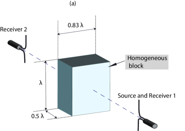
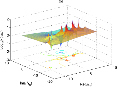
First we consider a homogeneous rectangular object of a resonant size depicted in Fig. 1 (a). The dimensions in terms of the free-space wavelength are indicated in the figure. The source of the incident field is an electric point-dipole situated one wavelength away from one the object faces. The dipole is polarized as shown in the figure. We simulate a single Cartesian component (indicated by the orientation of the receivers in the figure) of the scattered field, one wavelength away from the two opposite sides of the object, simulating the transmission and the backscattering measurement setups. The relative permittivity of the true object is $\varepsilon/\varepsilon_{0}=4$. The effective scatterer is also homogeneous and has the same outer shape. The discrepancy between the scattered field of the true object and the field scattered by homogeneous objects with other values of relative permittivity is shown as a surface in Fig. 1 (b), where the horizontal axes are the real and the imaginary parts of the trial relative permittivities, and the height of the surface gives the value of the discrepancy functional for Receiver 1. To visualize this functional on a $100\times 100$ grid we have computed the data-discrepancy for $K=10000$ different values of the complex relative permittivity, which would not be possible without a reduced-order algorithm discribed above.

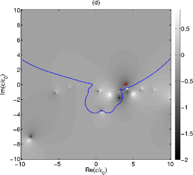
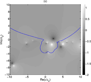
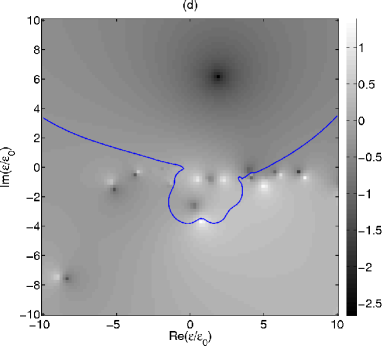
As expected from our theoretical analysis, the functional has many maxima and minima. Minima correspond to the match between the data, hence, giving the effective permittivities. Maxima, correspond to the singularities of (38), which, as predicted by equation (34), are situated in the lower half of the complex $(\varepsilon/\varepsilon_{0})$-plane and along the negative real axis. It is easier to analyze the shape of the functional on a two-dimensional image as the ones shown in Fig. 1 (c), (d), where the height of the functional is now represented by the brightness of the pixel. In these images bright spots correspond to singularities, and dark spots are the effective permittivities.

Also shown is a contour around an area of the $(\varepsilon/\varepsilon_{0})$-plane where the forward scattering problem is solved with sufficient accuracy. The norm of the residual of the forward problem is smaller than 0.01 inside the contour (here, above the curve), i.e. we have beteer than 1% accuracy there. The variation of accuracy with permittivity is the result of a fixed number of Arnoldi iterations applied everywhere (here and below we use $M=60$ iterations). We achieve an almost machine precision for small contrasts, i.e. for $\varepsilon/\varepsilon_{0}$ in the neighborhood of one, but arrive at progressively larger residuals for larger contrasts. Also, we cannot count on any good accuracy in the immediate neighborhood of discrete singularities and for all non-positive real $\varepsilon/\varepsilon_{0}$, as the forward problem becomes numerically ill-conditioned there. Achieving acceptable accuracy for larger areas of the $(\varepsilon/\varepsilon_{0})$-plane comes at a cost of more Arnoldi iterations, and in our case is limited to $M=60$ by the available computing resources. On the other hand, the depicted contour gives the norm of the residual of the forward problem, i.e. the total error in the solution all over the spatial doain $D$ and for all Cartesian components of the electric field. Whereas, what we should be concerned about is the error in the computed scattered field at the receiver location only. That error is probably much smaller than the norm of the residual on $D$. Therefore, we may expect that the computed reduced-order functionals can be trusted way beyond the outlined contour.

The different minima of the discrepancy functional, some in the “physical” part of the $(\varepsilon/\varepsilon_{0})$-plane, see Fig 1 (c), illustrate the non-uniqueness of the homogeneous effective model. If we compare Fig. 1 (c) and Fig. 1 (d), which correspond to different locations of the receiver, then we notice that all singularities remain at the same points, since they depend only on the shape of the scatterer and the applied frequency. At the same time all but one minima have changed their locations. The one which did not move was, of course, the permittivity of the original homogeneous object $\varepsilon/\varepsilon_{0}=4$. This gives us a way to retrieve the unique permittivity of a homogeneous scatterer from just two data-points via detection of a stationary minimum.

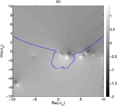
Application of the homogeneous effective model to an inhomogeneous elementary cell, similar to those used in photonic crystals Krowne2007 , is depicted in Fig. 2. We have two cylindrical rods, both with the relative permittivity $\varepsilon/\varepsilon_{0}=4$, and a $\lambda/3$ gap between their centers, see Fig. 2 (a).

Figure 2: An attempt to find the effective permittivity of an inhomogeneous object: (a) – scattering configuration; (b), (c), and (d) – data-discrepancy functionals for Receiver 1, Receiver 2, and Receiver 3, correspondingly. Notice the presence of two “physical” solutions in (b) and (d), demonstrating the non-uniqueness, and the absence of a “stationary” minimum in (b)–(d), demonstrating the non-existence of the exact effective permittivity for inhomogeneous objects.

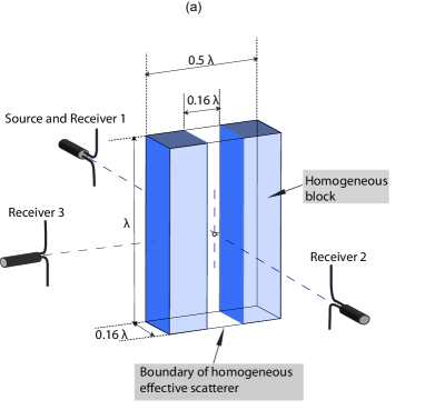
We consider three different locations of the receiver, indicated in Fig. 2-a as Receiver 1, Receiver 2, and Receiver 3, correspondingly. The distance of all receivers to the nearest faces of the scatterer is set to one wavelength. Both the true and the effective objects are smaller with respect to the wavelength than in the previous example (in the horizontal cross-section). Hence, we see less singularities and minima in the images of Fig. 2 (b), (c), and (d). The other significant difference is the absence of a minimum, stationary with respect to the changes in the measurement setup. This illustrates the anticipated non-existence of the exact effective permittivity in the inhomogeneous case.

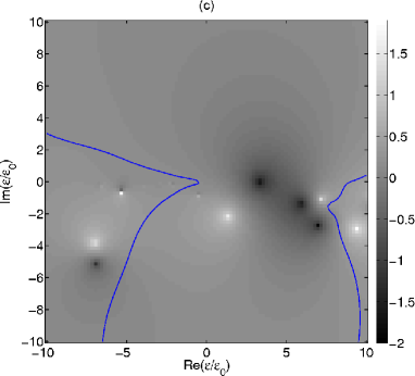
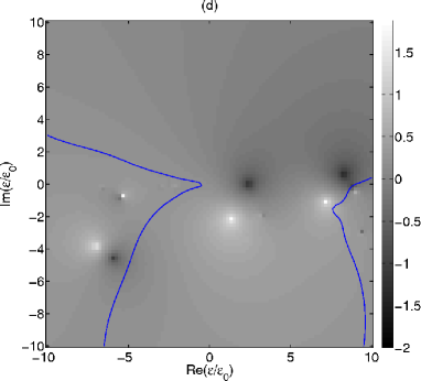
Finally we consider a larger sample of a dielectric photonic crystal, similar to the one investigated in Krowne2007 in relation to the phenomenon of negative refraction. In Fig. 3 (a) the scattering configuration is shown, where all three receivers are one wavelength away from the corresponding faces of the rectangular effective object. This effective model has, in fact, the same dimensions as the one considered in Fig 1.

Figure 3: An attempt to find the effective permittivity of a larger photonic-crystal sample: (a) – scattering configuration; (b), (c), and (d) – data-discrepancy functionals for Receiver 1, 2, and 3, correspondingly. Although this crystal is built out of the elementary cells considered in Fig. 2, the effective permittivities are now different as they are influenced by the geometry of the sample, which has the same dimensions as the homogeneous object considered in Fig. 1.

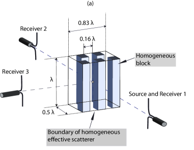
The frequency is chosen in such a way that the cyliners in Fig. 3 (a) form a triangular photonic lattice in the horizontal cross-section with the lattice period equal to $\lambda/3$. Thus, we are in the vicinity of the bandgap for this lattice, which might be the reason behind the large losses exhibited by one of the effective permittivity minima, see Fig. 3 (d). Otherwise there are still multiple minima for each separate receiver location, and no stationary minima. Also the minima of Fig. 2 and Fig. 3 are different, showing that the effective permittivity depends on the geometry and size of the sample. Of course, it would be interesting to see, if there is a convergence in the location of the minima for progressively larger pieces of this photonic crystal. Unfortunately, we were not able to investigate this question, due to the limitations imposed on us by the computing resources.

The Arnoldi algorithm used in Budko2004 and here is still a little too costly in terms of computer memory as it requires storage of $M$ vectors of size $N$, which are used as a basis for the total field. The reason for this choice of a robust but computationally expensive algorithm is the non-normal complex-symmetric system matrix of our problem. A possible alternative based on the Pade via Lanczos process was proposed in Remis2006 for the two-dimensional effective inversion problem. It requires storage of only three vectors of size $N$. A further generalization of the method, suitable for inhomogeneous scattering models and working with the Maxwell equations in their differential form was proposed in Druskin2007 .

We have presented here only a few examples which illustrate the main conclusions of the theoretical part of this paper. In addition, we have performed a large number of numerical experiments with different types of objects, looked at different field components, tried different types of incident fields (plane waves and Gaussian beams), considered measurements in the far-field zone, etc. Every time we would get images quite similar to the ones presented here, with a large number of virtually unpredictable minima. Except for the low frequencies, where within the considered range of permittivities we would typically get only one minimum, which was more or less stable with respect to the receiver location. When we considered a larger sample of a photonic crystal (7 rows, 12–13 cylindrical rods in each) at a very low frequency, then the observed minimum was in a close agreement with the effective permittivity predicted by the Maxwell-Garnet mixing formula.

V Conclusions

We have presented a generalization of the S-parameter retrieval method to three-dimensional finite objects and arbitrary illumination and observation conditions. We view it as a special kind of inverse scattering problem – an effective inversion problem. Many, if not all, conclusions of this paper equally apply to the S-parameter retrieval technique, the original low-frequency effective medium theory, and even to the derivation of the macroscopic Maxwell equations, as we have shown here the mathematical equivalence of all these problems up to the form of averaging/scattering operators. Of course, analysis in 3D is much more complicated and implicit than in 1D, where an explicit analytical solution for a homogeneous slab is available. Nevertheless, straightforward application of the spectral analysis and basic results from the inverse scattering theory showed that the general 3D case is similar to the well-studied 1D slabs in many respects.

The “exact” effective permittivity, which provides the exact match between the scattered field from an effective homogeneous object and the original inhomogeneous one, exists only on a limited set of incident fields and a limited number of observation points (angles). In fact, we can only be sure about the existence of this exact effective permittivity, either “physical” or not, when we have a single incident field and a single component of the scattered field observed at a single spatial location. We have shown that addition of just one more observation location may already cause the non-existence of the exact effective permittivity. On the other hand, addition of sources and/or receivers may lead to the uniqueness of an approximate effective permittivity (although we are not able to prove it yet). However, the more data we take into account the more approximate (less accurate) an effective model becomes. Also, the approximate effective permittivity is geometry-dependent, making it difficult to view metamaterials and other strongly inhomogeneous composites as continuous media suitable for carving out arbitrarily-shaped optical devices.

The exact effective permittivity, if it exists, is non-unique. As was shown here, this is due to the non-linearity of the effective inversion problem and the nontrivial null-space of the scattered-field operator. In the single data-point case, the number of additional exact effective permittivities depends on the spatial spectrum of the incident field – the broader this spectrum, the more non-unique is the solution of the problem. The spatial spectrum here is the spectrum of the scattering operator, rather than the usual plane waves. An incident plane wave has, in fact, a very broad spatial spectrum. The location of additional solutions in the complex plane is determined by the incident field and the spectrum of the scattering operator and is pretty arbitrary. Hence, it is not always possible to choose one of the solutions on some “physical” grounds.

The effective inversion problem becomes singular for certain values of effective permittivity. Many of them lie in the “non-physical” area of the complex plane and show negative loss. As such they do not cause much trouble. However, real nonpositive values of the effective permittivity important for negative refraction and invisibility must be excluded as well, as for those values the solution of the forward scattering problem either does not exist, or is not unique, or both. Luckily, the location of singularities depends only on the applied frequency and the outer shape of the object and does not depend on the illumination/observation conditions.

Although we have expressed some scepticism about the usefulness of effective models that are more complex than the original scatterer, we consider this topic to be worth pursuing. For example, it is imperative to know if there exists a complete-data set, perhaps, larger than the boundary data of the Calderón problem, such that would guarantee the uniqueness of the solution of the inverse scattering problem for a general inhomogeneous anisotropic scatterer. Also, the formal difference between the effective inversion method and the effective medium (and macroscopic electrodynamics) approach, although small, needs to be considered in more detail. Even with respect to the completely equivalent (double-averaged) EMT we do not know if there are conditions ensuring the uniqueness of the averaged inverse problem (19). Thus, depending on the actual form of the averaging operator $B$, it may still turn out that the problems of the EMT and the macroscopic electrodynamics have exact solutions under the illumination conditions which preclude the existence of the solution of the effective inversion (S-parameter retrieval) problem.

References

- (1) T. C. Choy, Effective medium theory, Claredon Press, Oxford, 1999.
- (2) C. F. Bohren, Applicability of effective-medium theories to problems of scattering and absorption by nonhomogeneous atmospheric particles, Journal of the Atmospheric Sciences 43, 468 – 475, 1985.
- (3) D. R. Smith, S. Schultz, P. Markos, and C. M. Soukoulis, Determination of effective permittivity and permeability of metamaterials from reflection and transmission coefficients, Phys. Rev. B 65, 195104, 2002.
- (4) D. Seetharamdoo, R. Sauleau, K. Mahdjoubi, and A.-C. Tarot, Effective parameters of resonant negative refractive index metamaterials: Interpretation and validity, J. Appl. Phys. 98, 063505, 2005.
- (5) B.-I. Popa and S. A. Cummer, Determining the effective electromagnetic properties of negative-refractive-index metamaterials from internal fields, Phys. Rev. B 72, 165102, 2005.
- (6) D. R. Smith, D. C. Vier, Th. Koschny, and C. M. Soukoulis, Electromagnetic parameter retrieval from inhomogeneous metamaterials, Phys. Rev. E 71, 036617, 2005.
- (7) X. Chen, B.-I. Wu, J. A. Kong, and T. M. Grzegorczyk, Retrieval of the effective constitutive parameters of anisotropic metamaterials, Phys. Rev. E 71, 046610, 2005.
- (8) D. Wang, J. Huangfu, L. Ran, H. Chen, T. M. Grzegorczyk, and J. A. Kong, Measurement of negative permittivity and permeability from experimental transmission and reflection with effects of cell misalignment, J. Appl. Phys 99, 123114, 2006.
- (9) V. V. Varadan and A. R. Tellakula, Effective properties of split-ring resonator metamaterials using measured scattering parameters: Effect of gap orientation, J. Appl. Phys. 100, 034910, 2006.
- (10) D. R. Smith and J. B. Pendry, Homogenization of metamaterials by field averaging (invited paper), J. Opt. Soc. Am. B 23, 391–403, 2006.
- (11) A. Pimenov and A. Loidl, Conductivity and permittivity of two-dimensional metallic photonic crystals, Phys. Rev. Lett. 96, 063903, 2006.
- (12) X. Chen, T. M. Grzegorczyk, and J. A. Kong, Optimization approach to the retrieval of the constitutive parameters of a slab of general bianisotropic medium, Progress In Electromagnetic Research, PIER 60, 1–18, 2006.
- (13) J. Song, W. Zhao, Q. H. Fu, and X. P. Zhao, Two-peak property in assymetric left-handed metamaterials, J. Appl. Phys. 101, 023702, 2007.
- (14) E. Saenz, P. M. T. Ikonen, R. Gonzalo, and S. A. Tretyakov, On the definition of effective permittivity and permeability for thin composite layers, J. Appl. Phys. 101, 112910, 2007.
- (15) V. Fokin, M. Ambati, C. Sun, and X. Zhang, Method for retrieving effective properties of locally resonant metamaterials, Phys. Rev. B 76, 144302, 2007.
- (16) G. Lubkowski, R. Schuhmann, and T. Weiland, Extraction of effective metamaterial parameters by parameter fitting of dispersive models, Microw. Opt. Techn. Lett. 49, 285–288, 2007.
- (17) A. P. Vinogradov, A. V. Dorofeenko, and S. Zouhdi, On the problem of the effective parameters of metamaterials, Physics - Uspekhi 51, 485–492, 2008.
- (18) J. Zhou, T. Koschny, M. Kafesaki, and C. M. Soukoulis, Size dependence and convergence of the retrieval parameters of metamaterials, Photonics and Nanostructures - Funamentals and Applications 6, 96–101, 2008.
- (19) W. Smigaj and B. Gralak, Validity of the effective-medium approximation of photonic crystals, Phys. Rev. B 77, 235445, 2008.
- (20) D.-H. Kwon, D. H. Werner, A. V. Kildishev, and V. M. Shalaev, Material parameter retrieval procedure for general bi-isotropic metamaterials and its application to optical chiral negative-index metamaterial design, Optics Express 16, 11822–11829, 2008.
- (21) A. I. Cabuz, D. Felbacq, and D. Cassagne, Spatial dispersion in negative-index composite metamaterials, Phys. Rev. A 77, 013807, 2008.
- (22) C. Menzel, C. Rockstuhl, T. Paul, F. Lederer, and T. Pertsch, Retrieving effective parameters for metamaterials at obligue incidence, Phys. Rev. B 77, 195328, 2008.
- (23) C. Menzel, C. Rockstuhl, T. Paul, and F. Lederer, Retrieving effective parameters for quasiplanar chiral metamaterials, Appl. Phys. Lett. 93, 233106, 2008.
- (24) U. C. Hasar, Elimination of the multple-solutions ambiguity in permittivity extraction from trasmission-only measurements of lossy materials, Microw. Opt. Techn. Lett. 51, 337–341, 2009.
- (25) J. Jin, S. Liu, Z. Lin, and S. T. Chui, Effective-medium theory for anisotropic magnetic materials, Phys. Rev. B 80, 115101, 2009.
- (26) C. Tserkezis, Effective parameters for periodic photonic structures of resonant elements, J. Phys.: Condens. Matter 21, 155404(7pp), 2009.
- (27) Z. Li, K. Aydin, amd E. Ozbay, Determination of the effective constitutive parameters of bianisotropic metamaterials from reflection and transmission coefficients, Phys. Rev. E 79, 026610, 2009.
- (28) S. Sun, S. T. Chui, and L. Zhou, Effective-medium properties of metamaterials: A quasimode theory, Phys. Rev. E 79, 066604, 2009.
- (29) R.-L. Chern and Y.-T. Chen, Effective parameters for photonic crystals with large dielectric constant, Phys. Rev. B 80, 075118, 2009.
- (30) V. Tyagi and E. Smouchkina, Sensittivity analysis of the effective parameter extraction procedure for metamaterial applications, Microw. Opt. Techn. Lett. 51, 1013–1017, 2009.
- (31) C. Menzel, T. Paul, C. Rockstuhl, F. Lederer, T. Pertsch, and S. A. Tretyakov, May metamaterials be described by effective material parameters?, arXiv:0908.2393, 2009.
- (32) A. Andyieuski, R. Malureanu, and A. V. Lavrinenko, Wave propagation retrieval method for metamaterials: Unambigous restoration of effective parameters, arXiv:0909.2134, 2009.
- (33) J. Rahola, On the eigenvalues of the volume integral operator of electromagnetic scattering, SIAM J. Sci. Comput. 21, 1740–1754, 2000.
- (34) A. B. Samokhin, Integral Equations and Iteration Methods in Electromagnetic Scattering, VSP, Utrecht, The Netherlands, 2001.
- (35) M. A. Yurkin and A. G. Hoekstra, The discrete dipole approximation: An overview and recent developments, Journal of Quantitative Spectroscopy and Radiative Transfer 106, 558–589, 2007.
- (36) S. G. Mikhlin and S. Prössdorf, Singular integral operators, Springer-Verlag, Berlin, 1980.
- (37) D. Colton and R. Kress, Inverse acoustic and electromagnetic scattering theory, Springer-Verlag, 1992.
- (38) A. P. M. Zwamborn and P. M. van den Berg, The three-dimensional weak form of the conjugate gradient FFT method for solving scattering problems, IEEE Trans. Microwave Theory Tech. 40, 1757–1766, 1992.
- (39) D. Colton and L. Päivärinta, The uniqueness of a solution to and inverse scattering problem for electromagnetic waves, Arch. Rational Mech. Anal. 119, 59–70, 1992.
- (40) M. C. van Beurden, Integro-differential equations for electromagnetic scattering, Ph.D. Thesis, Technische Universiteit Eindhoven, 2003.
- (41) N. V. Budko and A. B. Samokhin, Spectrum of the volume integral operator of electromagnetic scattering, SIAM J. Sci. Comput. 28, 682–700, 2006.
- (42) R. E. Kleinman, G. F. Roach, and P. M. van den Berg, Convergent Born series for large refractive indices, J. Opt. Soc. Amer. A 7, 890–897, 1990.
- (43) N. V. Budko and A. B. Samokhin, Singular modes of the electromagnetic field, J. Phys. A: Math. Theor. 40, 6239–6250, 2007.
- (44) L. N. Trefethen and M. Embree, Spectra and Pseudospectra: The Behavior of Nonnormal Matrices and Operators, Princeton, NJ: Princeton University Press, 2005.
- (45) N. V. Budko and A. B. Samokhin, Classification of electromagnetic resonances in finite inhomogeneous three-dimensional structures, Phys. Rev. Lett. 96, 023904, 2006.
- (46) D. G. Dudley, T. M. Habashy, and E. Wolf, Linear inverse problems in wave motion: nonsymmetric first-kind integral equations, IEEE Transactions on Antennas and Propagation 48, 1607–1617, 2000.
- (47) N. V. Budko and P. M. van den Berg, Two-dimensional object characterization with an effective model, Journal of Electromagnetic Waves and Applications 12, 177–190, 1998.
- (48) N. V. Budko and P. M. van den Berg, Characterization of a two-dimensional subsurface object with an effective scattering model, IEEE Trans. Geosc. and Remote Sensing 37, 2585–2596, 1999.
- (49) A. Greenleaf, Y. Kurylev, M. Lassas, and G. Uhlmann, Invisibility and inverse problems, Bulletin of the AMS 46, 55-97, 2008.
- (50) V. Druskin, On the uniqueness of inverse problems from incomplete boundary data, SIAM Journal on Applied Mathematics 58, 1591–1603, 1998.
- (51) B. Harrach, On uniqueness in diffuse optical tomography, Inverse Problems 25, 055010, 2009.
- (52) N. V. Budko, A. B. Samokhin, and A. A. Samokhin, A generalized overrelaxation method for solving singular volume integral equations in low-frequency scattering problems, Differential Equations 41, 1262–1266, 2005.
- (53) A. Greenleaf, Y. Kurylev, M. Lassas, and G. Uhlmann, Electromagnetic wormholes and virtual magnetic monopoles from metamaterials, Phys. Rev. Lett. 99, 183901, 2007.
- (54) N. V. Budko, Linearized electromagnetic inversion of inhomogeneous media with dispersion, Inverse Problems 18, 1509–1523, 2002.
- (55) N. V. Budko and R. F. Remis, Electromagnetic inversion using a reduced-order three-dimensional homogeneous model, Inverse Problems 20, S17–S26, 2004.
- (56) E. Ozbay and G. Ozkan, Negative refraction and subwavelength focusing in two-dimensional photonic crystals, in Physics of negative refraction and negative index materials, C. F. Krowne and Y. Zhang (eds.), Springer Series in Materials Science 98, Springer, 2007.
- (57) R. F. Remis, An effective inversion method based on the Pade via Lanczos process, Progress in Electromagnetics Research Online 2, 206–209, 2006.
- (58) V. Druskin and M. Zaslavsky, On combining model reduction and Gauss-Newton algorithms for inverse partial differential equation problems, Inverse Problems 23, 1599–1610, 2007.