Lattès maps and finite subdivision rules

Abstract.

This paper is concerned with realizing Lattès maps as subdivision maps of finite subdivision rules. The main result is that the Lattès maps in all but finitely many analytic conjugacy classes can be realized as subdivision maps of finite subdivision rules with one tile type. An example is given of a Lattès map which is not the subdivision map of a finite subdivision rule with either i) two tile types and 1-skeleton of the subdivision complex a circle or ii) one tile type.

This paper is concerned with realizing rational maps by subdivision maps of finite subdivision rules. If $\mathcal{R}$ is an orientation-preserving finite subdivision rule such that the subdivision complex $S_{\mathcal{R}}$ is a 2-sphere, then the subdivision map $\sigma_{\mathcal{R}}$ is a postcritically finite branched map. Furthermore, $\mathcal{R}$ has bounded valence if and only if $\sigma_{\mathcal{R}}$ has no periodic critical points. In [1] and [4], Bonk-Meyer and Cannon-Floyd-Parry prove that if $f$ is a postcritically finite rational map without periodic critical points, then every sufficiently large iterate of $f$ is the subdivision map of a finite subdivision rule $\mathcal{R}$ with two tile types such that the 1-skeleton of $S_{\mathcal{R}}$ is a circle. Since finite subdivision rules are essentially combinatorial objects, this gives good combinatorial models for these iterates. It is especially convenient to realize a postcritically finite map by the subdivision map of a finite subdivision rule with either a single tile type or with two tile types and 1-skeleton of the subdivision complex a circle.

While passing to an iterate is not usually a serious obstacle, it would be preferable if one didn’t need to do this. Suppose $f$ is a postcritically finite rational map without periodic critical points. We consider the following questions.

1. Is $f$ the subdivision map of a finite subdivision rule?

2. Is $f$ the subdivision map of a finite subdivision rule with two tile types and 1-skeleton of the subdivision complex a circle?

3. Is $f$ the subdivision map of a finite subdivision rule with one tile type?

In this paper we consider these questions for Lattès maps. The main result of this paper is to answer question 3 in the affirmative for the maps in all but finitely many analytic conjugacy classes of Lattès maps. In addition we exhibit a Lattès map of degree 2 for which the answer to questions 2 and 3 is negative, although the answer to question 1 is positive.

This paper has four sections. The first section develops the setting of Lattès maps. These results can be used to easily enumerate all Lattès maps of very small degree to test (not so easy) the above three questions for them.

Section 2 presents the pruning lemma and immediate consequences. To describe the pruning lemma, let $f$ be a Lattè$s$ map which is the subdivision map of a finite subdivision rule with one tile type. This obtains a subdivision complex structure on the Riemann sphere whose 1-skeleton is a tree. The postcritical points of $f$ are vertices of this tree. The pruning lemma states that it is possible to prune this tree to obtain a subtree for which every vertex with valence either 1 or 2 is a postcritical point and this subtree is the 1-skeleton of a subdivision complex for which $f$ is the subdivision map. So if $f$ is the subdivision map for a subdivision complex whose 1-skeleton is a tree, then $f$ is the subdivision map for a subdivision complex whose 1-skeleton is a tree with a special form. This special form is very restrictive.

Section 3 contains the main result in Corollary 3.11, namely, that every map in almost every analytic conjugacy class of Lattès maps is the subdivision map of a finite subdivision rule with one tile type. This is essentially proved in two theorems. The first theorem, Theorem 3.1, states that every Lattès map with sufficiently large degree is the subdivision map of a finite subdivision rule with one tile type. The second theorem, Theorem 3.10, states that every nonrigid Lattès map is the subdivision map of a finite subdivision rule with one tile type. Since there are only finitely many analytic conjugacy classes of rigid Lattès maps with a given degree (See the end of Section 1.), these two theorems give the main result. Theorems 3.1 and 3.10 actually say a bit more, giving additional information about the tilings.

The proof of Theorem 3.1 is much more difficult than the proof of Theorem 3.10. It roughly parallels the proof of the main theorem of [4]. The strategy is to construct a finite subdivision rule $\mathcal{R}$ with one tile type, bounded valence, and mesh approaching 0 combinatorially such that the subdivision map $\sigma_{\mathcal{R}}$ of $\mathcal{R}$ is isotopic to the Lattès map $f$ relative to its postcritical set $P_{f}$. Once this is achieved, our results for expansion complexes [3] can be used to show that $\sigma_{\mathcal{R}}$ and $f$ are in fact conjugate rel $P_{f}$, and so $f$ is the subdivision map of a finite subdivision rule with one tile type. The finite subdivision rule $\mathcal{R}$ is constructed using a lift of $f$ to the complex plane and a standard tiling of the plane by regular hexagons. Our tiling of the Riemann sphere by one tile lifts to a tiling of the plane which is combinatorially equivalent to this standard tiling by regular hexagons. The proof of Theorem 3.10 does not require an isotopy and hence does not require results for expansion complexes. In this case our tiling of the Riemann sphere by one tile lifts to a standard tiling of the plane by parallelograms.

Section 4 presents an example which shows that the main result does not hold for every Lattès map. This example is a quadratic Lattès map $f$ for which both question 2 and question 3 are false. Question 1 is true for $f$, as we show that $f$ is the subdivision map of a finite subdivision rule with two tile types, but the 1-skeleton of the subdivision complex is not a circle. The Lattès map $f$ has a lift to the complex plane of the form $\widetilde{f}(z)=\alpha z$, where $\alpha=(1+\sqrt{-7})/2$ and the postcritical set of $f$ lifts to the lattice generated by 1 and $\alpha$. The complex conjugate of $f$ gives another such example. Yet another example with these properties is given by a real cubic Lattès map $g$. The map $g$ has a lift to the complex plane of the form $\widetilde{g}(z)=\alpha z$, where $\alpha=\sqrt{-3}$ and the postcritical set of $g$ lifts to the lattice generated by 1 and $(1+\sqrt{-3})/2$. It is possible to prove these claims for $g$ much as we prove them for $f$ in Section 4. The three analytic conjugacy classes of Lattès maps represented by these three maps are probably the only ones for which question 3 is false.

As for question 1, as far as we know, every rational map with finite postcritical set and no periodic critical points is the subdivision map of a finite subdivision rule.

1. Definitions and basic facts for Lattès maps

Following Milnor [7, Remark 3.5], we define a Lattès map to be a rational function from the Riemann sphere $\widehat{\mathbb{C}}$ to itself such that its local degree at every critical point is 2 and there are exactly four postcritical points, none of which is also critical. Let $f\colon\thinspace\widehat{\mathbb{C}}\to\widehat{\mathbb{C}}$ be a Lattès map.

As in Section 3.1 of [7], it follows that there exists an analytic branched cover $\wp\colon\thinspace\mathbb{C}\to\widehat{\mathbb{C}}$ which is branched exactly over the postcritical points of $f$ and the local degree of $\wp$ at every branch point is 2. (The function $\wp$ is a Weierstrass $\wp$-function up to precomposing and postcomposing with analytic automorphisms.) Let $\Lambda$ be the set of branch points of $\wp$. It is furthermore true that $\wp$ is a regular branched cover, and its group of deck transformations $\Gamma$ is generated by the set of all rotations of order 2 about the points of $\Lambda$. We refer to $\Gamma$ as the orbifold fundamental group of $f$. Given rotations $z\mapsto 2\lambda-z$ and $z\mapsto 2\mu-z$ of order 2 about the points $\lambda,\mu\in\Lambda$, their composition, the second followed by the first, is the translation $z\mapsto z+2(\lambda-\mu)$. We may, and do, normalize so that $0\in\Lambda$. So $\Gamma$ contains a subgroup with index 2 consisting of translations of the form $z\mapsto z+2\lambda$ with $\lambda\in\Lambda$. It follows that $\Lambda$ is a lattice in $\mathbb{C}$ and that the elements of $\Gamma$ are the maps of the form $z\mapsto\pm z+2\lambda$ for some $\lambda\in\Lambda$.

Douady and Hubbard show in [6, Proposition 9.3] that the map $f\colon\thinspace\widehat{\mathbb{C}}\to\widehat{\mathbb{C}}$ lifts to a map $\widetilde{f}\colon\thinspace\mathbb{C}\to\mathbb{C}$ given by $\widetilde{f}(z)=\alpha z+\beta$ for some imaginary quadratic algebraic integer $\alpha$ (possibly an element of $\mathbb{Z}$) such that $\alpha\Lambda\subseteq\Lambda$ and some $\beta\in\Lambda$. The following lemma is devoted to determining to what extent $\alpha$, $\beta$, and $\Lambda$ are determined by the analytic conjugacy class of $f$.

Lemma 1.1.

Let $f_{0}$ be a Lattès map which is analytically conjugate to $f$. Let $\wp_{0}\colon\thinspace\mathbb{C}\to\widehat{\mathbb{C}}$ be a branched cover for $f_{0}$ corresponding to $\wp$. Let $\Lambda_{0}$ be the set of branch points of $\wp_{0}$, and assume that $0\in\Lambda_{0}$. Suppose that $f_{0}\colon\thinspace\widehat{\mathbb{C}}\to\widehat{\mathbb{C}}$ lifts to a map $\widetilde{f}_{0}\colon\thinspace\mathbb{C}\to\mathbb{C}$ given by $\widetilde{f}_{0}(z)=\alpha_{0}z+\beta_{0}$. Then the following hold.

1. $\alpha_{0}=\pm\alpha$.

2. $\beta_{0}=\gamma\beta+\delta$ where $\gamma\in\mathbb{C}^{\times}$ and $\delta\in(\alpha+1)\Lambda_{0}+2\Lambda_{0}$.

3. $\Lambda_{0}=\gamma\Lambda$ with $\gamma$ as in statement 2.

Conversely, if $\wp_{0}\colon\thinspace\mathbb{C}\to\widehat{\mathbb{C}}$ is a branched cover as above, if $\Lambda_{0}$ is the set of branch points of $\wp_{0}$ with $0\in\Lambda_{0}$, and if $\widetilde{f}_{0}(z)=\alpha_{0}z+\beta_{0}$ such that statements 1, 2, and 3 hold, then $\widetilde{f}_{0}$ is the lift of a Lattè$s$ map which is analytically conjugate to $f$.

Proof.

Let $\sigma$ be a Möbius transformation such that $f_{0}=\sigma\circ f\circ\sigma^{-1}$. Just as for $f$ and $f_{0}$, the map $\sigma\colon\thinspace\widehat{\mathbb{C}}\to\widehat{\mathbb{C}}$ lifts to a map $\widetilde{\sigma}\colon\thinspace\mathbb{C}\to\mathbb{C}$ given by $\widetilde{\sigma}(z)=\rho z+\nu$ for some $\rho\in\mathbb{C}^{\times}$ and $\nu\in\mathbb{C}$. Since $\sigma$ maps the postcritical set of $f$ to the postcritical set of $f_{0}$, $\widetilde{\sigma}$ maps $\Lambda$ to $\Lambda_{0}$, that is, $\rho\Lambda+\nu=\Lambda_{0}$. In other words, the coset $\rho\Lambda+\nu$ of the group $\rho\Lambda$ equals the group $\Lambda_{0}$. The only way that a coset can be a group is if it is the trivial coset, and so $\nu\in\Lambda_{0}$ and $\Lambda_{0}=\rho\Lambda$. Since $\widetilde{f}_{0}$ and $\widetilde{\sigma}\circ\widetilde{f}\circ\widetilde{\sigma}^{-1}$ are both lifts of $f_{0}$, they differ by an element of $\Gamma_{0}$, the group of deck transformations of $\wp_{0}$. In other words, there exists $\lambda_{0}\in\Lambda_{0}$ such that $\pm\widetilde{f}_{0}(z)+2\lambda_{0}=\widetilde{\sigma}\circ\widetilde{f}\circ\widetilde{\sigma}^{-1}(z)$ for all $z\in\mathbb{C}$. So we have the following.

$$\pm(\alpha_{0}z+\beta_{0})+2\lambda_{0} =\pm\widetilde{f}_{0}(z)+2\lambda_{0}=\widetilde{\sigma}\circ\widetilde{f}\circ\widetilde{\sigma}^{-1}(z)=\rho\widetilde{f}(\rho^{-1}(z-\nu))+\nu$$

$$=\rho(\alpha\rho^{-1}(z-\nu)+\beta)+\nu=\alpha z+\rho\beta+(1-\alpha)\nu$$

Hence $\alpha_{0}=\pm\alpha$, which yields statement 1. Furthermore

$$\pm\beta_{0}=\rho\beta+(1-\alpha)\nu-2\lambda_{0}.$$

We have seen that $\nu\in\Lambda_{0}$. So setting $\gamma=\pm\rho$ and $\delta=\pm((\alpha+1)\nu-2\alpha\nu-2\lambda_{0})$, we have that $\beta_{0}=\gamma\beta+\delta$ with $\gamma\in\mathbb{C}^{\times}$ and $\delta\in(\alpha+1)\Lambda_{0}+2\Lambda_{0}$. We now have verified statements 1, 2, and 3.

For the converse, it is a straightforward matter to construct $\widetilde{\sigma}$ such that $\widetilde{\sigma}$ conjugates $\widetilde{f}$ to $\widetilde{f}_{0}$ up to the action of $\Gamma_{0}$. One checks that $\widetilde{\sigma}$ descends to a rational map $\sigma\colon\thinspace\widehat{\mathbb{C}}\to\widehat{\mathbb{C}}$ which has local degree 1 at every point of $\widehat{\mathbb{C}}$. So $\sigma$ is a Möbius transformation. It follows that $\widetilde{f}_{0}$ is the lift of an analytic conjugate of $f$.

This completes the proof of Lemma 1.1.

∎

Lemma 1.1 implies that with an appropriate modification of $\beta$ the lattice $\Lambda$ may be replaced by $\gamma\Lambda$, where $\gamma$ is any nonzero complex number, without changing the analytic conjugacy class of $f$. In Section 7 of Chapter 2 of the number theory book [2] by Borevich and Shafarevich the lattices $\Lambda$ and $\gamma\Lambda$ are said to be similar. Theorem 9 and the remark following it in Section 7 of Chapter 2 of [2] imply that every lattice in $\mathbb{C}$ is similar to a lattice with a $\mathbb{Z}$-basis consisting of 1 and $\tau$, where $\tau$ lies in the standard fundamental domain for the action of $\text{SL}(2,\mathbb{Z})$ on the upper half complex plane. More precisely, $\tau$ satisfies the following inequalities.

(1.2) $$\begin{gathered}\text{Im}(\tau)>0\\ -\frac{1}{2}<\text{Re}(\tau)\leq\frac{1}{2}\\ |\tau|\geq 1\,\text{ and if }|\tau|=1,\text{ then }\text{Re}(\tau)\geq 0\end{gathered}$$

Moreover there is only one such $\tau$ which satisfies these inequalities. This and Lemma 1.1 imply that $\tau$ is uniquely determined by the analytic conjugacy class of $f$.

Corollary 1.3.

Let $\widetilde{f}_{0}(z)=\alpha_{0}z+\beta_{0}$ be a linear polynomial such that $\widetilde{f}_{0}(\Lambda)\subseteq\Lambda$. Then $\widetilde{f}_{0}$ descends via the branched cover $\wp\colon\thinspace\mathbb{C}\to\widehat{\mathbb{C}}$ to a rational function which is analytically conjugate to $f$ if and only if $\alpha_{0}=\pm\alpha$ and $\beta_{0}=\gamma\beta+\delta$ where $\gamma\Lambda=\Lambda$, $\gamma=e^{\pm 2\pi i/n}$ with $n\in\{1,2,3,4,6\}$, and $\delta\in(\alpha+1)\Lambda+2\Lambda$.

Proof.

In this situation $\Lambda_{0}=\Lambda$. So just as for $\widetilde{f}$, the containment $\gamma\Lambda\subseteq\Lambda$ implies that the complex number $\gamma$ is in fact an imaginary quadratic algebraic integer. Because $\gamma\Lambda=\Lambda$, $\gamma$ is invertible, that is, it is a unit. But all imaginary quadratic units have the form $e^{\pm 2\pi i/n}$ with $n\in\{1,2,3,4,6\}$. This discussion and Lemma 1.1 prove Corollary 1.3.

∎

In this paragraph we consider related effects of complex conjugation. It is easy to see that the complex conjugate of a Lattès map is also a Lattès map. By applying complex conjugation to the Lattès map $f$, the branched cover $\wp$, and the lift $\widetilde{f}$ of $f$, we see that the complex conjugate of $\widetilde{f}$ is a lift of the complex conjugate of $f$. With respect to finite subdivision rules, the behavior of $f$ is the same as the behavior of $\overline{f}$, so when considering $\widetilde{f}(z)=\alpha z+\beta$, we may assume that $\text{Im}(\alpha)\geq 0$. Since $\widetilde{f}$ and $-\widetilde{f}$ both lift $f$, we may also assume that $\text{Re}(\alpha)\geq 0$. This shows that the restrictions put on $\alpha$ in the following lemma are reasonable.

Lemma 1.4.

As above, let $\Lambda$ be the inverse image in $\mathbb{C}$ of the postcritical set of the Lattès map $f\colon\thinspace\widehat{\mathbb{C}}\to\widehat{\mathbb{C}}$, and let $\widetilde{f}(z)=\alpha z+\beta$ be a lift of $f$. Suppose that 1 and $\tau$ form a $\mathbb{Z}$-basis of $\Lambda$. Multiplication by $\alpha$ determines an endomorphism of $\Lambda$. Let $\left[\begin{matrix}a&b\\ c&d\end{matrix}\right]$ be the matrix of this endomorphism with respect to the ordered $\mathbb{Z}$-basis $(1,\tau)$. Suppose that $\text{Im}(\alpha)>0$. Then $\text{Re}(\alpha)\geq 0$ and $\tau$ lies in the standard fundamental domain for the action of $\text{SL}(2,\mathbb{Z})$ on the upper half complex plane if and only if the following inequalities are satisfied.

$$\begin{gathered}c>0\\ a\geq-\frac{c}{2}\\ \max\{a-c+1,-a\}\leq d\leq a+c\\ b\leq-c\,\text{ and if }\,b=-c,\text{ then }d\geq a\end{gathered}$$

Proof.

From the first column of the matrix $\left[\begin{matrix}a&b\\ c&d\end{matrix}\right]$ it follows that $\alpha=a+c\tau$. So $\tau=\frac{\alpha-a}{c}$. The matrix of the endomorphism determined by $\alpha-a$ is $\left[\begin{matrix}0&b\\ c&d-a\end{matrix}\right]$. Because the eigenvalues of this matrix are $\alpha-a$ and $\overline{\alpha-a}$, its trace is twice the real part of $\alpha-a$ and its determinant is the square of the modulus of $\alpha-a$. So $\text{Re}(\alpha-a)=\frac{d-a}{2}$ and $|\alpha-a|^{2}=-bc$. Hence $\text{Re}(\tau)=\frac{d-a}{2c}$ and $|\tau|^{2}=-\frac{b}{c}$. Similarly $\text{Re}(\alpha)=\frac{a+d}{2}$.

Suppose that $\text{Re}(\alpha)\geq 0$ and that the inequalities in line 1.2 hold. Since $\tau=\frac{\alpha-a}{c}$ and $\text{Im}(\alpha)>0$, the inequality $\text{Im}(\tau)>0$ implies that $c>0$, giving the first inequality in the statement of the lemma. For the second inequality, we combine $\text{Re}(\alpha)\geq 0$ and $\text{Re}(\tau)\leq\frac{1}{2}$ to obtain $a+d\geq 0$ and $d-a\leq c$, hence $a-d\geq-c$. So $a\geq-\frac{c}{2}$, giving the second inequality in the statement of the lemma. Combining $-\frac{1}{2}<\text{Re}(\tau)\leq\frac{1}{2}$ and $\text{Re}(\alpha)\geq 0$ obtains $-c<d-a\leq c$ and $a+d\geq 0$, which easily gives the third inequality in the statement of the lemma. The fourth inequality follows from the fact that $|\tau|\geq 1$ with equality only if $\text{Re}(\tau)\geq 0$.

Proving the converse is straightforward.

This proves Lemma 1.4.

∎

Lemma 1.5.

(1) In Corollary 1.3 the case $\gamma=\pm i$ occurs only when $\tau=i$, and the case $\gamma=\pm e^{\pm 2\pi i/3}$ occurs only when $\tau=e^{2\pi i/6}$.
(2) Let $\left[\begin{matrix}a&b\\ c&d\end{matrix}\right]$ be as in Lemma 1.4, and let $M$ be the reduction of $\left[\begin{matrix}a+1&b\\ c&d+1\end{matrix}\right]$ modulo 2. Then a complete list of distinct coset representatives of $(\alpha+1)\Lambda+2\Lambda$ in $\Lambda$ is given by

$$\begin{gathered}0\text{ if }\text{rank}(M)=2\\ 0,1,\tau,\tau+1\text{ if }\text{rank}(M)=0\\ 0,\lambda\text{ if }\text{rank}(M)=1,\end{gathered}$$

where $\lambda$ is any element of $\Lambda$ whose image in $\Lambda/2\Lambda$ is not in the column space of $M$.

Proof.

If $\gamma=\pm i$, then $i\in\Lambda$ because $\gamma\Lambda\subseteq\Lambda$. But then $i$ is an integral linear combination of 1 and $\tau$ with $\tau$ in the standard fundamental domain for the action of $\text{SL}(2,\mathbb{Z})$ on the upper half complex plane. This implies that $\tau=i$. A similar argument applies when $\gamma=\pm e^{\pm 2\pi i/3}$. This proves statement 1.

Statement 2 is clear.

∎

Since the elements of the orbifold fundamental group are Euclidean isometries, $\widetilde{f}$ multiplies areas uniformly by the factor $\deg(f)$. Translation by $\beta$ does not change areas. Multiplication by $\alpha$ multiplies lengths by $\left|\alpha\right|$ and areas by $\left|\alpha\right|^{2}=\alpha\overline{\alpha}$. Multiplication by $\alpha$ also corresponds to multiplication by the matrix $\left[\begin{matrix}a&b\\ c&d\end{matrix}\right]$, and this multiplies areas by its determinant. Therefore $\deg(f)=\alpha\overline{\alpha}=ad-bc$.

Lemma 1.6.

If $a$, $b$, $c$, and $d$ satisfy the inequalities of Lemma 1.4, then $ad-bc\geq 3c^{2}/4$.

Proof.

The inequalities of Lemma 1.4 imply that $\left|a-d\right|\leq c$. Hence $c^{2}\geq(a-d)^{2}\geq(a-d)^{2}-(a+d)^{2}=-4ad$. Since $b\leq-c$ and $c>0$, it follows that $ad-bc\geq-c^{2}/4+c^{2}=3c^{2}/4$, as desired.

∎

Let $f$ be a Lattès map with lift $\widetilde{f}(z)=\alpha z+\beta$ and lattice $\Lambda$ as above. We say that $f$ is nonrigid if $\alpha\in\mathbb{R}$, equivalently, $\alpha\in\mathbb{Z}$. We say that $f$ is rigid if $\alpha\notin\mathbb{R}$. If $f$ is nonrigid, then since multiplication by an integer stabilizes every lattice in $\mathbb{C}$, $\Lambda$ can be arbitrary. There are uncountably many analytic conjugacy classes of Lattès maps for every integer $\alpha\geq 2$. On the other hand, there are only finitely many analytic conjugacy classes of rigid Lattès maps with a given degree. To see why, first note that Lemma 1.6 and the paragraph before it imply that in the rigid case a bound on $\deg(f)=ad-bc$ puts a bound on $c$. We may assume that $\text{Im}(\alpha)>0$. The inequalities of Lemma 1.4 imply that a bound on $c$ puts a lower bound on $a$ and $d$. Because $b\leq-c$, $c>0$ and $\left|a-d\right|\leq c$, a bound on $ad-bc$ puts an upper bound on both $a$ and $d$. So a bound on $ad-bc$ puts a bound on $c$, $a$, $d$ and therefore $b$. So if $\deg(f)$ is bounded, then there are only finitely many possibilities for $a$, $b$, $c$ and $d$. These values determine $\alpha$ in the upper half plane and $\tau$. Given $\alpha$ and $\tau$, there are always at most four possibilities for $\beta$ up to equivalence. So if $f$ is rigid and $\deg(f)$ is bounded, then there are only finitely many possibilities for the analytic conjugacy class of $f$.

2. The pruning lemma

Suppose that the Lattès map $f$ is the subdivision map of a finite subdivision rule with one tile type. Then the 1-skeleton of our subdivision complex is a tree $T$ in $\widehat{\mathbb{C}}$. The object of the next lemma, the pruning lemma, is to prune $T$ in order to simplify our finite subdivision rule. Since $f$ is a homeomorphism on open cells of the subdivision complex, all postcritical points are vertices of $T$. The pruning lemma implies that we may assume that all other vertices of $T$ have valence at least 3. This lemma generalizes to more general maps and graphs, but for simplicity we content ourselves with the following statement.

Figure 1. The possible trees and tilings.

Lemma 2.1 (Pruning Lemma).

Suppose that the Lattès map $f$ is the subdivision map of a finite subdivision rule with one tile type. Then $f$ is the subdivision map of a finite subdivision rule with one tile type such that every vertex in its subdivision complex with valence either 1 or 2 is a postcritical point.

Proof.

Let $T$ be the 1-skeleton of the given finite subdivision rule. We temporarily view $T$ just as a topological space with no regard to vertices or edges. Let $S$ be the subspace of $T$ which is the union of all arcs joining postcritical points. Then $S$ is connected and hence is a topological tree. We next show that $f(S)\subseteq S$. For this, let $\gamma$ be an arc in $T$ joining two postcritical points. If the restriction of $f$ to $\gamma$ is injective, then $f(\gamma)$ is an arc joining two postcritical points, and so $f(\gamma)\subseteq S$. If the restriction of $f$ to $\gamma$ is not injective, then because $f$ maps $\gamma$ into the tree $T$ there exists a point $p\in\gamma$ such that $f(\gamma)$ is folded at $f(p)$. But then $p$ is a critical point and $f(p)$ is a postcritical point. We see that in general $f(\gamma)$ is a union of arcs which join two postcritical points. So $f(S)\subseteq S$. We make $S$ into a graph by putting vertices at the postcritical points as well as the points whose complements have at least three connected components. We see that $S$ is the 1-skeleton of a cell structure for the 2-sphere and that $f$ is a subdivision map for this subdivision complex with one tile type. The vertices of $S$ with valence either 1 or 2 are postcritical points.

This proves Lemma 2.1.

∎

Lemma 2.1 shows that if the Lattès map $f$ is the subdivision map of a finite subdivision rule with one tile type and 1-skeleton $T$, then we may assume that every vertex of $T$ with valence either 1 or 2 is a postcritical point. We refer to the vertices of $T$ which are not postcritical points as accidental vertices. The assumption that accidental vertices have valence at least 3 severely limits the possibilities for $T$. There are five of them. Figure 1 shows all five possibilities for $T$. The tile in $\widehat{\mathbb{C}}$ which $T$ determines lifts to a tiling of $\mathbb{C}$, and Figure 1 indicates the tiling corresponding to every possibility for $T$. Dots in trees indicate postcritical points, and dots in tilings indicate inverse images of postcritical points.

We emphasize that the illustrations in Figure 1 are correct only up to isotopy. This is true in particular for the tilings. The inverse image $\Lambda$ of the postcritical set of $f$ is a lattice and the tiling is invariant under the orbifold fundamental group $\Gamma$, which imposes a certain structure, but otherwise every tiling is correct only up to an affine transformation followed by a $\Gamma$-invariant isotopy rel $\Lambda$.

3. Main Results

Theorem 3.1.

Every Lattès map with sufficiently large degree is the subdivision map of a finite subdivision rule with one tile type, and the tile has the form of type 5 in Figure 1.

Proof.

The proof begins by fixing notation and making definitions. Then we outline the argument. Finally we fill in the details.

Let $f\colon\thinspace\widehat{\mathbb{C}}\to\widehat{\mathbb{C}}$ be a Lattès map. Let $\Lambda$ be a lift of the postcritical set of $f$, let $\widetilde{f}(z)=\alpha z+\beta$ be a lift of $f$, and let $\Gamma$ be the orbifold fundamental group as in Section 1. As in the paragraph immediately before Lemma 1.4, we may assume that $\text{Re}(\alpha)\geq 0$ and $\text{Im}(\alpha)\geq 0$. As in the paragraph containing line 1.2, we may assume that $\Lambda$ is a lattice with a $\mathbb{Z}$-basis consisting of 1 and $\tau$, where $\tau$ satisfies the inequalities in line 1.2; that is, we may assume that $\tau$ lies in the standard fundamental domain for the action of $\text{SL}(2,\mathbb{Z})$ on the upper half complex plane.

Since 1 and $\tau$ are linearly independent over $\mathbb{R}$, so are $\alpha^{-1}$ and $\alpha^{-1}\tau$. So there exists an $\mathbb{R}$-linear isomorphism $\psi\colon\thinspace\mathbb{C}\to\mathbb{C}$ such that the points of the lattice $\psi(\alpha^{-1}\Lambda)$ are midpoints of edges of a standard tiling $T$ of the plane by regular hexagons and 0, $\psi(\alpha^{-1})$, and $\psi(\alpha^{-1}\tau)$ lie in one hexagon as shown in Figure 2. Let $T^{*}$ be the tiling of the plane by equilateral triangles which is dual to $T$. The vertices of $T^{*}$ are the centers of the tiles of $T$. The duality between $T$ and $T^{*}$ determines a bijection between the edges of $T$ and the edges of $T^{*}$. Let $S$ and $S^{*}$ be the tilings of the plane which are the pullbacks of $T$ and $T^{*}$ under $\psi$.

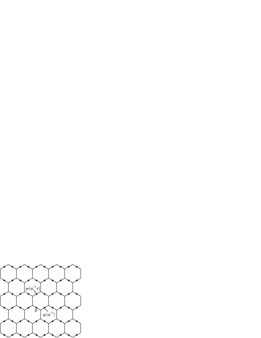
Figure 2. The tiling $T$.

In this paragraph we consider approximations to lines in the plane by edge paths in $S$. Let $L$ be a line in the plane, and first suppose that $L$ does not contain a vertex of $S^{*}$. We construct a subset $\widehat{L}$ of the plane as a union of edges of $S$. An edge $e$ of $S$ is contained in $\widehat{L}$ if and only if $L$ meets the edge of $S^{*}$ dual to $e$. See Figure 3, which shows part of $S$ and $S^{*}$. The dots indicate points of the lattice $\alpha^{-1}\Lambda$. Part of $L$ is shown, and part of $\widehat{L}$ is drawn with thick line segments. It is not difficult to see that $\widehat{L}$ is homeomorphic to $\mathbb{R}$. If $L$ contains a vertex but not an edge of $S^{*}$, then we construct $\widehat{L}$ in essentially the same way by perturbing $L$ near every vertex of $S^{*}$ contained in $L$. If $L$ is a union of edges of $S^{*}$, then we perturb every edge in $L$ to a new line segment whose endpoints are not vertices of $S^{*}$. The result is again a subset of the 1-skeleton of $S$ which is homeomorphic to $\mathbb{R}$, but in this case there are two choices for every vertex of $S^{*}$ in $L$ and $\widehat{L}$ is not unique. We call $\widehat{L}$ the edge path approximation to $L$.

Figure 3. Constructing the edge path approximation of the line $L$.

We now outline the proof of Theorem 3.1. See Figure 4. Let $L_{1}$ be the line containing $\beta$ and $1+\beta$. Since $\beta\in\Lambda$, either $L_{1}$ contains the centers of both tiles of $S$ which contain $\beta$ or $L_{1}$ does not contain the center of either tile of $S$ which contains $\beta$. If $L_{1}$ does not contain the centers of the two tiles of $S$ which contain $\beta$, then $\widehat{L}_{1}$ contains $\beta$. If $L_{1}$ contains the centers of the two tiles of $S$ which contain $\beta$, then $\widehat{L}_{1}$ is not uniquely determined, but we may choose $\widehat{L}_{1}$ so that it contains $\beta$. So we may assume that $\widehat{L}_{1}$ contains $\beta$, and likewise $1+\beta$. Let $L_{2}$ be the line containing $\tau+\beta$ and $1+\tau+\beta$. As for $\widehat{L}_{1}$, we may assume that $\widehat{L}_{2}$ contains both $\tau+\beta$ and $1+\tau+\beta$. We will later prove that $\widehat{L}_{1}$ and $\widehat{L}_{2}$ are usually disjoint. Let $L_{3}$ be the line containing $-\frac{1}{2}+\beta$ and $-\frac{1}{2}+\tau+\beta$. Let $P_{1}$ and $P_{2}$ be points of $\widehat{L}_{1}\cap\widehat{L}_{3}$ and $\widehat{L}_{2}\cap\widehat{L}_{3}$, respectively, such that the open segment of $\widehat{L}_{3}$ with endpoints $P_{1}$ and $P_{2}$ is disjoint from both $\widehat{L}_{1}$ and $\widehat{L}_{2}$. We will later prove that $P_{1}$ is usually strictly between $-1+\beta$ and $\beta$ in $\widehat{L}_{1}$ and that $P_{2}$ is usually strictly between $-1+\tau+\beta$ and $\tau+\beta$ in $\widehat{L}_{2}$. Let $Q_{1}$ be the image of $P_{1}$ under the rotation of order 2 about $\beta$, and let $R_{1}$ be the image of $Q_{1}$ under the rotation of order 2 about $1+\beta$. When $\widehat{L}_{1}$ is uniquely determined, the rotation of order 2 about any point of $\Lambda\cap L_{1}$ stabilizes $\widehat{L}_{1}$. When $\widehat{L}_{1}$ is not uniquely determined, we construct $\widehat{L}_{1}$ by making choices between $\beta$ and $1+\beta$ and then extending so that the rotation of order 2 about any point of $\Lambda\cap L_{1}$ stabilizes $\widehat{L}_{1}$. We construct $\widehat{L}_{2}$ in the same way. So $Q_{1}$ is a point of $\widehat{L}_{1}$ usually strictly between $\beta$ and $1+\beta$ and $R_{1}$ is a point of $\widehat{L}_{1}$ usually strictly between $1+\beta$ and $2+\beta$. The composition of two rotations of order 2 is a translation. We translate $L_{3}$ by the map $z\mapsto z+R_{1}-P_{1}$ to a line $L_{4}$. The image of the closed segment of $\widehat{L}_{3}$ with endpoints $P_{1}$ and $P_{2}$ under this translation is the closed segment of $\widehat{L}_{4}$ with endpoints $R_{1}$ and $R_{2}$. We will later prove that the closed segment of $\widehat{L}_{3}$ with endpoints $P_{1}$ and $P_{2}$ is usually disjoint from its image under this translation. From the segment of $\widehat{L}_{1}$ joining $P_{1}$ and $R_{1}$, the segment of $\widehat{L}_{4}$ joining $R_{1}$ and $R_{2}$, the segment of $\widehat{L}_{2}$ joining $R_{2}$ and $P_{2}$, and the segment of $\widehat{L}_{3}$ joining $P_{2}$ and $P_{1}$ we obtain the hatched region $F$, which is a union of tiles of $S$. Let $S^{\prime}$ be the tiling gotten from $S$ simply by making the points of $\Lambda$ vertices. So the vertices of $S$ are the vertices of $S^{\prime}$ with valence 3, and the points of $\Lambda$ are the vertices of $S^{\prime}$ with valence 2. Whereas the tiles of $S$ are hexagons, the tiles of $S^{\prime}$ are decagons. Let $s$ be the tile of $S^{\prime}$ containing 0, $\alpha^{-1}$, $\alpha^{-1}\tau$, and $\alpha^{-1}+\alpha^{-1}\tau$. There is a canonical pairing of the edges of $s$. The two edges of $s$ containing $0$ are interchanged by the rotation of order 2 about $0$. The same is true at $\alpha^{-1}$, $\alpha^{-1}\tau$, and $\alpha^{-1}+\alpha^{-1}\tau$. The two remaining edges of $s$ are translates of one another. In the same way we view $F$ as having six vertices $P_{1}$, $Q_{1}$, $R_{1}$, $P_{2}$, $Q_{2}$, $R_{2}$ of valence 3 and four vertices $\beta$, $1+\beta$, $\tau+\beta$, $1+\tau+\beta$ of valence 2, which we view as decomposing the boundary of $F$ into ten edges. The two edges of $F$ containing $\beta$ are interchanged by the rotation of order 2 about $\beta$. The same is true at $1+\beta$, $\tau+\beta$, and $1+\tau+\beta$. The two remaining edges of $F$ are translates of one another. It follows that $F$ is a fundamental domain for the orbifold fundamental group $\Gamma$. The image of every tile of $S^{\prime}$ under $\widetilde{f}$ is isotopic rel $\Lambda$ to the image of $F$ under some element of $\Gamma$, and these isotopies can be made $\Gamma$-equivariant. Because $f$ respects the edge pairings of $s$ and $F$ up to isotopy, when we descend to $\widehat{\mathbb{C}}$, the tiling of $F$ by the tiles of $S^{\prime}$ determines a finite subdivision rule $\mathcal{R}$ with one tile type. The subdivision rule $\mathcal{R}$ has bounded valence, in fact valences of vertices are bounded by 3. We will prove that the mesh of $\mathcal{R}$ usually approaches 0 combinatorially. The result is a finite subdivision rule $\mathcal{R}$ with bounded valence and mesh approaching 0 combinatorially such that the subdivision map $\sigma_{\mathcal{R}}$ of $\mathcal{R}$ is isotopic to $f$ rel $P_{f}$. From here we proceed as in the proof of the main theorem of [4] to conclude that $\sigma_{\mathcal{R}}$ and $f$ are in fact conjugate rel $P_{f}$, and so $f$ is the subdivision map of a finite subdivision rule with one tile type.

Figure 4. Constructing a fundamental domain when $\alpha=\frac{9+\sqrt{-23}}{2}$ and $\tau=\frac{-1+\sqrt{-23}}{4}$.

The previous paragraph reduces the proof of Theorem 3.1 to the construction of an appropriate fundamental domain $F$ for the orbifold fundamental group $\Gamma$. This in turn reduces to verifying certain claims made in the previous paragraph. The word “usually” occurs a few times. “Usually” means that the degree of $f$ is sufficiently large and that $\alpha\notin\{\tau,1+\tau,2+\tau\}$. The claims in the previous paragraph do not always hold if $\alpha\in\{\tau,1+\tau,2+\tau\}$ and sometimes when they do, the proofs below do not. The cases in which $\alpha\in\{\tau,1+\tau,2+\tau\}$ will be handled separately at the end of the proof. When edge path approximations are not unique, the claims mean that it is possible to choose edge path approximations so that the claims are true.

In this paragraph we make an observation concerning a type of symmetry. The outline in the next-to-last paragraph constructs a fundamental domain $F$ for the Lattès map with lift $z\mapsto\alpha z+\beta$ and lattice generated by 1 and $\tau$. The rotation of order 2 about $1+\tau+\beta$ takes $F$ to the corresponding fundamental domain for the Lattès map with lift $z\mapsto\alpha z+1+\tau+\beta$ and lattice generated by 1 and $\tau$. So for example, by this symmetry if for a fixed $\alpha$ and $\tau$ and for every $\beta\in\Lambda$ no tile of $S^{\prime}$ meets an edge of $F$ containing $\beta$ and an edge of $F$ containing $\tau+\beta$, then for the same fixed $\alpha$ and $\tau$ and for every $\beta\in\Lambda$ no tile of $S^{\prime}$ meets an edge of $F$ containing $1+\beta$ and an edge of $F$ containing $1+\tau+\beta$. We will use this symmetry to simplify arguments.

We prepare to verify the claims in the outline by turning our attention to edge path approximations.

Lemma 3.2.

Let $L$ and $L^{\prime}$ be parallel lines in the plane.

1. If no edge of $S^{*}$ meets both $L$ and $L^{\prime}$, then $\widehat{L}$ and $\widehat{L}^{\prime}$ are disjoint.

2. If there does not exist a line segment which is the union of two adjacent edges of $S^{*}$ such that this line segment meets both $L$ and $L^{\prime}$, then no tile of $S^{\prime}$ meets both $\widehat{L}$ and $\widehat{L}^{\prime}$.

Proof.

Note that because the vertices of $S$ have valence 3, if $\widehat{L}$ and $\widehat{L}^{\prime}$ are not disjoint, then they have an edge of $S$ in common. With this observation statement 1 follows from the definition of edge path approximation. To prove statement 2, let $L^{\prime\prime}$ be the line parallel to both $L$ and $L^{\prime}$ such that $L^{\prime\prime}$ is equidistant to $L$ and $L^{\prime}$. Suppose that there does not exist a line segment which is the union of two adjacent edges of $S^{*}$ such that this line segment meets both $L$ and $L^{\prime}$. Then no edge of $S^{*}$ meets both $L$ and $L^{\prime\prime}$. Likewise no edge of $S^{*}$ meets both $L^{\prime}$ and $L^{\prime\prime}$. So statement 1 implies that $\widehat{L}$, $\widehat{L}^{\prime}$, and $\widehat{L}^{\prime\prime}$ are mutually disjoint. Moreover $\widehat{L}^{\prime\prime}$ is between $\widehat{L}$ and $\widehat{L}^{\prime}$. It follows that no tile of $S^{\prime}$ meets both $\widehat{L}$ and $\widehat{L}^{\prime}$.

This proves Lemma 3.2.

∎

Lemma 3.3.

If the degree of $f$ is sufficiently large, then no tile of $S^{\prime}$ meets both $\widehat{L}_{1}$ and $\widehat{L}_{2}$.

Proof.

We prepare to apply statement 2 of Lemma 3.2. We consider whether or not there exists a line segment which is the union of two adjacent edges of $S^{*}$ such that this line segment meets both $L_{1}$ and $L_{2}$. First suppose that these two edges of $S^{*}$ are translates of the line segment joining 0 and $2\alpha^{-1}$. Since $\tau+\beta\in L_{2}$ and $L_{1}$ is the translate of the real axis by $\beta$, for such edges we are led to consider real numbers $r$ and $s$ such that $\tau+\beta+2r\alpha^{-1}=s+\beta$, that is, $\tau+2r\alpha^{-1}=s$. If $\alpha\in\mathbb{R}$, then there are no such numbers $r$ and $s$ and there is no such line segment which meets both $L_{1}$ and $L_{2}$. Otherwise $r$ and $s$ exist, and if $\left|r\right|>2$, then there does not exist such a line segment which meets both $L_{1}$ and $L_{2}$. The equation $\tau+2r\alpha^{-1}=s$ implies that $\alpha=r\frac{2}{s-\tau}$. Since $\text{Im}(\tau)$ is bounded from 0, the complex number $s-\tau$ is bounded from 0 uniformly in $\tau$ as $s$ varies over $\mathbb{R}$. So $r\frac{2}{s-\tau}$ is bounded uniformly in $\tau$ for $\left|r\right|\leq 2$ and $s\in\mathbb{R}$. Hence $\alpha$ is bounded for $\left|r\right|\leq 2$ and $s\in\mathbb{R}$. But since $\text{deg}(f)=\alpha\overline{\alpha}$, it follows that there is no such line segment meeting both $L_{1}$ and $L_{2}$ if the degree of $f$ is sufficiently large.

In addition to having edges in the direction of $2\alpha^{-1}$, the tiling $S^{*}$ has edges in the direction of $\alpha^{-1}(1+\tau)$ and $\alpha^{-1}(-1+\tau)$. We next perform analogous verifications for these edges. Once these verifications are complete, we may conclude that no tile of $S^{\prime}$ meets both $\widehat{L}_{1}$ and $\widehat{L}_{2}$ if the degree of $f$ is sufficiently large.

Now we consider edges of $S^{*}$ in the direction of $\alpha^{-1}(1+\tau)$. In this case we obtain the equation $\tau+r\alpha^{-1}(1+\tau)=s$. So $\alpha=r\frac{1+\tau}{s-\tau}$. For all real numbers $s$ we have that

(3.4) $$\left|s-\tau\right|\geq\text{Im}(\tau)=\left|\tau\right|\sin(\arg(\tau))\geq\frac{\sqrt{3}}{2}\left|\tau\right|,$$

and so

$$\left|\frac{1+\tau}{s-\tau}\right|\leq\frac{2}{\sqrt{3}}\frac{1+\left|\tau\right|}{\left|\tau\right|}\leq\frac{4}{\sqrt{3}}.$$

So $r\frac{1+\tau}{s-\tau}$ is bounded for $\left|r\right|\leq 2$ and $s\in\mathbb{R}$. Again it follows that there is no such line segment meeting both $L_{1}$ and $L_{2}$ if the degree of $f$ is sufficiently large.

For edges of $S^{*}$ in the direction of $\alpha^{-1}(-1+\tau)$ we replace $1+\tau$ by $-1+\tau$ in the previous paragraph and again conclude that there is no such line segment meeting both $L_{1}$ and $L_{2}$ if the degree of $f$ is sufficiently large. Thus if the degree of $f$ is sufficiently large, then no tile of $S^{\prime}$ meets both $\widehat{L}_{1}$ and $\widehat{L}_{2}$.

This proves Lemma 3.3.

∎

As in Figure 4, let $L_{5}$ be the line containing $\beta$ and $\tau+\beta$ and let $L_{6}$ be the line containing $1+\beta$ and $1+\tau+\beta$. It would be convenient to have a lemma for $L_{5}$ and $L_{6}$ analogous to Lemma 3.3 for $L_{1}$ and $L_{2}$. Unfortunately, the situation for $L_{5}$ and $L_{6}$ is more complicated than for $L_{1}$ and $L_{2}$. This takes us to the following two lemmas.

Lemma 3.5.

Let $L$ and $L^{\prime}$ be lines in the plane parallel to $L_{5}$ such that the distance between $L$ and $L^{\prime}$ is at least half the distance between $L_{5}$ and $L_{6}$. If the degree of $f$ is sufficiently large, then no line segment which is the union of two edges of $S^{*}$ in the direction of $\alpha^{-1}$ meets both $L$ and $L^{\prime}$.

Proof.

We consider whether or not there exists a line segment meeting both $L$ and $L^{\prime}$ which is the union of two edges of $S^{*}$ which are translates of the line segment joining 0 and $2\alpha^{-1}$. As in the proof of Lemma 3.3, we obtain the equation $x+2r\alpha^{-1}=s\tau$, and we wish to have no solution with $x\geq 1/2$, $|r|\leq 2$, and $s\in\mathbb{R}$. So we wish to have no solution to the equation $1+2r\alpha^{-1}=s\tau$ with $|r|\leq 4$ and $s\in\mathbb{R}$. Solving the last equation for $\alpha$ shows that $\alpha=r\frac{2}{s\tau-1}$. The argument in line 3.4 with $\tau^{-1}$ instead of $\tau$ shows for all real numbers $s$ that $\left|s-\tau^{-1}\right|\geq\frac{\sqrt{3}}{2}\left|\tau\right|^{-1}$, and so $\left|s\tau-1\right|\geq\frac{\sqrt{3}}{2}$. So $r\frac{2}{s\tau-1}$ is bounded uniformly in $\tau$ for $\left|r\right|\leq 4$ and $s\in\mathbb{R}$. Hence $\alpha$ is bounded for $\left|r\right|\leq 4$ and $s\in\mathbb{R}$. Since $\text{deg}(f)=\alpha\overline{\alpha}$, this proves that there is no such line segment if the degree of $f$ is sufficiently large.

This proves Lemma 3.5.

∎

Lemma 3.6.

Let $L$ and $L^{\prime}$ be lines in the plane parallel to $L_{5}$. Let $a$ and $c$ be the integers such that $\alpha=a+c\tau$.

1. If the distance between $L$ and $L^{\prime}$ is at least half the distance between $L_{5}$ and $L_{6}$ and if either $c\geq 11$ or $c=0$ with $a\geq 5$, then no line segment which is the union of two edges of $S^{*}$ in the direction of either $\alpha^{-1}(1+\tau)$ or $\alpha^{-1}(-1+\tau)$ meets both $L$ and $L^{\prime}$.

2. If the distance between $L$ and $L^{\prime}$ is at least twice the distance between $L_{5}$ and $L_{6}$, then usually no edge of $S^{*}$ in the direction of either $\alpha^{-1}(1+\tau)$ or $\alpha^{-1}(-1+\tau)$ meets both $L$ and $L^{\prime}$.

Proof.

We prove both statements together. We first consider edges of $S^{*}$ in the direction of $\alpha^{-1}(1+\tau)$. Arguing as in the proof of Lemma 3.5, we obtain the equation $1+r\alpha^{-1}(1+\tau)=s\tau$. For statement 1 we want there to be no solution in real numbers $r$ and $s$ with $\left|r\right|\leq 4$. For statement 2 the restriction on $r$ is $\left|r\right|\leq\frac{1}{2}$. Solving for $\alpha$ shows that $\alpha=-r\frac{1+\tau}{1-s\tau}$.

We justify every step of the next display immediately after it.

$$c\text{Im}(\tau)=\text{Im}(\alpha)\leq\left|\alpha\right|=\left|r\right|\left|\frac{1+\tau}{1-s\tau}\right|\leq\left|r\right|\frac{4\left|\tau\right|}{\sqrt{3}}\leq\left|r\right|\frac{8}{3}\text{Im}(\tau)$$

The two equations and the first inequality are straightforward. For the second inequality, we use the fact that $1\leq\left|\tau\right|$ to obtain $\left|1+\tau\right|\leq 1+\left|\tau\right|\leq 2\left|\tau\right|$. Using line 3.4 as in the proof of Lemma 3.5, we obtain $\left|1-s\tau\right|\geq\frac{\sqrt{3}}{2}$. Combining the results of the last two sentences gives the second inequality of the display. Line 3.4 implies that $\left|\tau\right|\leq\frac{2}{\sqrt{3}}\text{Im}(\tau)$. This gives the last inequality of the above display. From the display we conclude that $c\leq\left|r\right|\frac{8}{3}$. Hence if $\left|r\right|\leq 4$, then $c\leq\frac{32}{3}$ and if $\left|r\right|\leq\frac{1}{2}$, then $c\leq\frac{4}{3}$. This proves statement 1 for edges of $S^{*}$ in the direction of $\alpha^{-1}(1+\tau)$ except when $c=0$ and it proves statement 2 for edges of $S^{*}$ in the direction of $\alpha^{-1}(-1+\tau)$ except when $c\in\{0,1\}$.

To continue, we consider the image of the extended real line under the linear fractional transformation $z\mapsto\frac{1+\tau}{1-z\tau}$. One verifies that $\infty\mapsto 0$, $-1\mapsto 1$, and $0\mapsto 1+\tau$. Since linear fractional transformations map circles and extended lines to circles and extended lines, it follows that the image of the extended real line is the circle $C$ containing 0, 1, and $1+\tau$.

Thus if $\left|r\right|\leq 4$ and $c=0$, then $0<\alpha\leq 4$. This completes the proof of statement 1 for edges of $S^{*}$ in the direction of $\alpha^{-1}(1+\tau)$. If $\left|r\right|\leq\frac{1}{2}$ and $c=0$, then $0<\alpha\leq\frac{1}{2}$. Hence statement 2 is true for edges of $S^{*}$ in the direction of $\alpha^{-1}(1+\tau)$ if $c=0$.

It remains to prove statement 2 for edges of $S^{*}$ in the direction of $\alpha^{-1}(1+\tau)$ when $c=1$. Recall that $C$ contains 0, 1, and $1+\tau$. This implies that the center of $C$ is on the line given by $\text{Re}(z)=\frac{1}{2}$. Every point of the circle $C^{\prime}$ through 0 and 1 with center $\frac{1}{2}$ has imaginary part at most $\frac{1}{2}$. Since $\text{Im}(1+\tau)\geq\frac{\sqrt{3}}{2}>\frac{1}{2}$, the imaginary part of the center of $C$ is positive. Comparing $C$ with $C^{\prime}$, we see that no points of the form $a-\tau$ with $a\in\mathbb{R}$ are within $C$. Since $\text{Re}(1+\tau)>\frac{1}{2}$, the complex number $1+\tau$ is in the right half of $C$. So no complex number of the form $a+\tau$ with $a>1$ is within $C$. Hence no such number is within $\frac{1}{2}C$. Since “usually” means that $a\geq 3$ if $c=1$, this completes the proof of statement 2 for edges of $S^{*}$ in the direction of $\alpha^{-1}(1+\tau)$.

For edges of $S^{*}$ in the direction of $\alpha^{-1}(-1+\tau)$, we argue in the same way. The only modification occurs at the very end. Whereas before the circle $C$ contains $1+\tau$, now it contains $-1+\tau$. This is insufficient to conclude that no complex number of the form $a+\tau$ with $a>1$ is within $C$. For this we verify that the linear fractional transformation $z\mapsto\frac{-1+\tau}{1-z\tau}$ maps the real number $\frac{-1+\tau+\overline{\tau}}{\tau\overline{\tau}}$ to $-\overline{\tau}=-2\text{Re}(\tau)+\tau$. Now we can conclude that no complex number of the form $a+\tau$ with $a>1$ is within $C$.

This proves Lemma 3.6. ∎

We now consider the claims made in the outline of Theorem 3.1. The first claim is that $\widehat{L}_{1}$ and $\widehat{L}_{2}$ are usually disjoint. This follows from Lemma 3.3. The next claim is that $P_{1}$ is usually strictly between $-1+\beta$ and $\beta$ in $\widehat{L}_{1}$. This is the main content of the first statement of the next lemma. The other two statements are closely related results which will be used later.

Lemma 3.7.

(1) The point $P_{1}$ is usually strictly between $-1+\beta$ and $\beta$ in $\widehat{L}_{1}$ and $P_{1}$ is usually not adjacent to either $-1+\beta$ or $\beta$ in the tiling $S^{\prime}$.

1. Usually no tile of $S^{\prime}$ meets both $\widehat{L}_{3}$ between $P_{1}$ and $P_{2}$ and $\widehat{L}_{1}$ between $Q_{1}$ and $R_{1}$.

2. Usually no tile of $S^{\prime}$ meets both $\widehat{L}_{4}$ between $R_{1}$ and $R_{2}$ and $\widehat{L}_{1}$ between $P_{1}$ and $Q_{1}$.

Proof.

We prove all three statements together. As usual, let $a$ and $c$ be the integers such that $\alpha=a+c\tau$. We begin by proving Lemma 3.7 for either $c=0$ or $c\geq 11$. In this case statement 2 of Lemma 3.2, Lemma 3.5, and statement 1 of Lemma 3.6 combine to imply that usually no tile of $S^{\prime}$ meets both $\widehat{L}_{3}$ and $\widehat{L}_{5}$. (The condition in Lemma 3.6 that $a\geq 5$ can be met by taking the degree of $f$ to be sufficiently large.) Since $\beta\in L_{5}$, we may assume that $\beta\in\widehat{L}_{5}$. So we have that $\beta\in\widehat{L}_{1}\cap\widehat{L}_{5}$, and it is easy to see that the points of $\widehat{L}_{1}$ which are on the same side of $\beta$ as $1+\beta$ either lie on $\widehat{L}_{5}$ or are on the same side of $\widehat{L}_{5}$ as $1+\beta$. Since $\widehat{L}_{3}$ is usually strictly on the other side of $\widehat{L}_{5}$ and $P_{1}\in\widehat{L}_{3}$, it follows that $P_{1}$ is usually strictly on the same side of $\beta$ as $-1+\beta$ in $\widehat{L}_{1}$ and that $P_{1}$ is usually not adjacent to $\beta$ in $S^{\prime}$. This argument also shows that usually no tile of $S^{\prime}$ meets $\widehat{L}_{3}$ between $P_{1}$ and $P_{2}$ and $\widehat{L}_{1}$ between $Q_{1}$ and $R_{1}$. We have so far proved that $P_{1}$ is usually strictly on the same side of $\beta$ as $-1+\beta$ in $\widehat{L}_{1}$, that $P_{1}$ is usually not adjacent to $\beta$ in $S^{\prime}$, and that statement 2 is true if either $c=0$ or $c\geq 11$. Analogous arguments prove that $P_{1}$ is usually strictly on the same side of $-1+\beta$ as $\beta$ in $\widehat{L}_{1}$, that $P_{1}$ is usually not adjacent to $-1+\beta$ in $S^{\prime}$, and that statement 3 is true if either $c=0$ or $c\geq 11$. This proves Lemma 3.7 if either $c=0$ or $c\geq 11$.

So suppose that $1\leq c\leq 10$ for the rest of the proof of Lemma 3.7. We partition this case into two subcases according to whether $a<3c$ or $a\geq 3c$. Let $b$ and $d$ be the integers such that $\alpha\tau=b+d\tau$. If $a<3c$, then both $a$ and $c$ are bounded. With $a$ and $c$ bounded, Lemma 1.4 implies that $d$ is bounded. Because $\deg(f)=ad-bc$ and this degree may be taken to be arbitrarily large, the integer $b$ may be taken to be arbitrarily negative. So if $a<3c$, then $d$ is bounded and $b$ may be taken to be arbitrarily negative. On the other hand, if $a\geq 3c$, then Lemma 1.4 implies that $d>0$. Of course, $b<0$.

In this paragraph suppose that $a\geq 3c$. We will prove statement 2 and half of statement 1 under this assumption. Let $X=\{x\alpha^{-1}+y\alpha^{-1}\tau+\beta:x,y\in\mathbb{R},x\leq-\frac{3}{2}\}$, a closed half plane. Let $\overline{X}$ be the union of the tiles of $S^{\prime}$ contained in $X$. Both $\psi(\overline{X})$ and the image of $\psi(\overline{X})$ under the rotation of order 2 about $\psi(\beta)$ are shaded in Figure 5. There are essentially two possibilities, hence two parts to Figure 5, depending on whether the edge of $T$ containing $\psi(\beta)$ has negative or positive slope. It is possible to choose $\widehat{L}_{1}$ so that the portion of $\psi(\widehat{L}_{1})$ in the region shown in Figure 5 is contained in the hatched region which is pinched near $\psi(\beta)$. The lines $L_{1}$ and $L_{3}$ meet at $-\frac{1}{2}+\beta=-\frac{a}{2}\alpha^{-1}-\frac{c}{2}\alpha^{-1}\tau+\beta$, and this point is in $X$ since $a\geq 3c\geq 3$. Moreover, this point is in the boundary of $X$ if and only if $a=3$ and $c=1$. Since $b<0$, the half of $L_{3}$ with endpoint $-\frac{1}{2}+\beta$ which contains $-\frac{1}{2}+\tau+\beta=-\frac{1}{2}+b\alpha^{-1}+d\alpha^{-1}\tau+\beta$ is in $X$. So the half of $\widehat{L}_{3}$ with endpoint $P_{1}$ which contains $P_{2}$ is contained in $\overline{X}$. Similarly, the half of $\widehat{L}_{1}$ with endpoint $P_{1}$ which does not contain $\beta$ is contained in $\overline{X}$. So the half of $\widehat{L}_{1}$ with endpoint $Q_{1}$ which does not contain $\beta$ is contained in the image of $\overline{X}$ under the rotation of order 2 about $\beta$. We see that $P_{1}$ is strictly on the same side of $\beta$ as $-1+\beta$ in $\widehat{L}_{1}$ and that $P_{1}$ is not adjacent to $\beta$ in $S^{\prime}$. Moreover no tile of $S^{\prime}$ meets both $\widehat{L}_{3}$ between $P_{1}$ and $P_{2}$ and $\widehat{L}_{1}$ between $Q_{1}$ and $R_{1}$. We have just proved statement 2 and half of statement 1 when $1\leq c\leq 10$ and $a\geq 3c$.

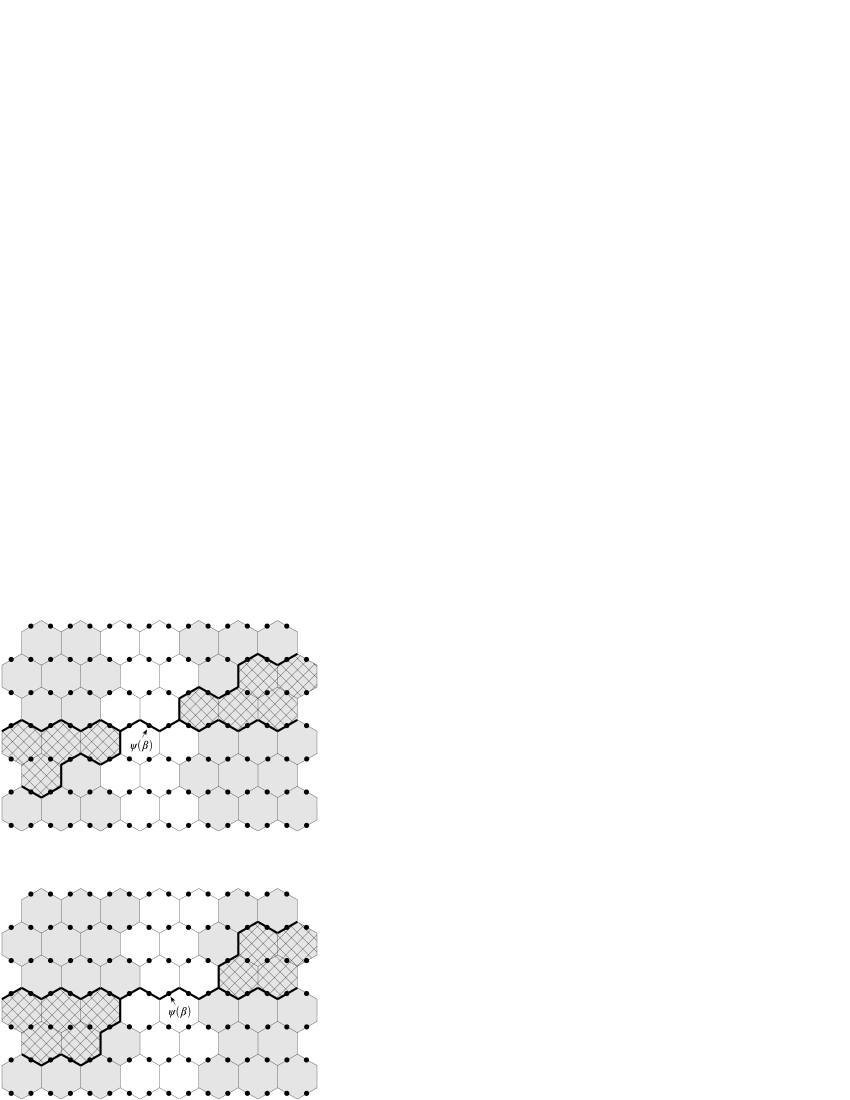
Figure 5. Proving Lemma 3.7.

Next suppose that $a<3c$. We will prove statement 2 and the same half of statement 1 under this assumption. Recall from the definition of usually that $\alpha\notin\{\tau,1+\tau,2+\tau\}$. This together with the inequality $a<3c$ implies that we may assume that $c\neq 1$. For every integer $m$ we consider the closed half plane $Y_{m}=\{x\alpha^{-1}+y\alpha^{-1}\tau+\beta:y\geq m-\frac{1}{2}\}$. Let $\overline{Y}_{m}$ be the union of the tiles of $S^{\prime}$ contained in $Y_{m}$. Now let $m$ be the ceiling of $-\frac{c}{2}$. Again $L_{1}$ and $L_{3}$ meet at $-\frac{1}{2}+\beta=-\frac{a}{2}\alpha^{-1}-\frac{c}{2}\alpha^{-1}\tau+\beta$. This point is in $Y_{m}$. Because $L_{3}$ contains $-\frac{1}{2}+\beta$ and $-\frac{1}{2}+\tau+\beta=-\frac{1}{2}+b\alpha^{-1}+d\alpha^{-1}\tau+\beta$ and because $d$ is bounded and $b$ can be made arbitrarily negative, the slope of $\psi(L_{3})$ can be made arbitrarily close to 0. The edge path distance between $-\frac{1}{2}+\beta$ and $P_{1}$ is bounded since $a$ and $c$ are bounded, so it follows that usually an arbitrarily long initial portion of the directed segment of $\widehat{L}_{3}$ from $P_{1}$ to $P_{2}$ is in the boundary of either $\overline{Y}_{m}$ or $\overline{Y}_{m-1}$. In particular, $P_{1}$ is usually in the boundary of either $\overline{Y}_{m}$ or $\overline{Y}_{m-1}$. Moreover since $c\geq 2$, it follows that $m<0$, and so $P_{1}\notin\overline{Y}_{0}$. Similarly, the half of $\widehat{L}_{1}$ with endpoint $P_{1}$ which does not contain $\beta$ is disjoint from $\overline{Y}_{0}$. On the other hand, $\beta\in\overline{Y}_{0}$, and the half of $\widehat{L}_{1}$ with endpoint $\beta$ which contains $1+\beta$ is even in $\overline{Y}_{0}$. The previous two sentences together with the fact that $Q_{1}$ is the image of $P_{1}$ under the rotation of order 2 about $\beta$ imply that the half of $\widehat{L}_{1}$ with endpoint $Q_{1}$ which does not contain $\beta$ is in $\overline{Y}_{1}$. Thus $P_{1}$ is usually strictly on the same side of $\beta$ as $-1+\beta$ in $\widehat{L}_{1}$, it is usually not adjacent to $\beta$ in $S^{\prime}$, and usually no tile of $S^{\prime}$ meets both $\widehat{L}_{3}$ between $P_{1}$ and $P_{2}$ and $\widehat{L}_{1}$ between $Q_{1}$ and $R_{1}$. This completes the proof of statement 2 and half of statement 1 when $1\leq c\leq 10$.

Finally we prove statement 3 and the other half of statement 1 when $1\leq c\leq 10$. As in the previous paragraph, it is still true that $-\frac{1}{2}+\beta$ is contained in $Y_{m}$, where $m$ is the ceiling of $-\frac{c}{2}$. It is also still usually true that $P_{1}$ is in $\overline{Y}_{n}$ with either $n=m$ or $n=m-1$. If $a\geq 3c$, then the slope of $\psi(L_{3})$ is negative and the directed segment of $\widehat{L}_{3}$ from $P_{1}$ to $P_{2}$ is also in $\overline{Y}_{n}$. If $a<3c$, then this slope might be negative, but usually an arbitrarily long initial portion of this directed segment is contained in $\overline{Y}_{n}$. Moreover, if $c\in\{1,2\}$, then $d\geq 0$, the slope of $\psi(L_{3})$ is nonpositive, and we may take $n=m$. It follows that $-c<n$ and that $-1+\beta\notin\overline{Y}_{n}$. It is also true that the half of $\widehat{L}_{1}$ with endpoint $P_{1}$ which contains $\beta$ is contained in $\overline{Y}_{n}$. The last two sentences combine to prove that $P_{1}$ is usually strictly on the same side of $-1+\beta$ as $\beta$ in $\widehat{L}_{1}$ and that $P_{1}$ is not adjacent to $-1+\beta$ in $S^{\prime}$. The translation $z\mapsto z+2=z+2a\alpha^{-1}+2c\alpha^{-1}\tau$ stabilizes $\widehat{L}_{1}$ and it takes the directed segment of $\widehat{L}_{3}$ from $P_{1}$ to $P_{2}$ to the directed segment of $\widehat{L}_{4}$ from $R_{1}$ to $R_{2}$. So either the directed segment of $\widehat{L}_{4}$ from $R_{1}$ to $R_{2}$ is contained in $\overline{Y}_{n+2c}$ or at least an arbitrarily long initial portion of it is usually contained in $\overline{Y}_{n+2c}$. Since $-1+b\notin\overline{Y}_{n}$, it follows that $1+\beta\notin\overline{Y}_{n+2c}$. Since the segment of $\widehat{L}_{1}$ between $P_{1}$ and $Q_{1}$ is contained in the image of $\overline{Y}_{n+2c}$ under the rotation of order 2 about $1+\beta$, it follows that usually no tile of $S^{\prime}$ meets both the segment of $\widehat{L}_{4}$ between $R_{1}$ and $R_{2}$ and the segment of $\widehat{L}_{1}$ between $P_{1}$ and $Q_{1}$.

This proves Lemma 3.7.

∎

So $P_{1}$ is usually strictly between $-1+\beta$ and $\beta$ in $\widehat{L}_{1}$. The next claim in the outline is that $P_{2}$ is usually strictly between $-1+\tau+\beta$ and $\tau+\beta$ in $\widehat{L}_{2}$. To see this, note that the previous claim and symmetry show that $R_{2}$ is usually strictly between $1+\tau+\beta$ and $2+\tau+\beta$ in $\widehat{L}_{2}$. This and a translation imply that $P_{2}$ is usually strictly between $-1+\tau+\beta$ and $\tau+\beta$ in $\widehat{L}_{2}$.

The next claim is that the closed segment of $\widehat{L}_{3}$ with endpoints $P_{1}$ and $P_{2}$ is usually disjoint from its image under the translation given by $z\mapsto z+R_{1}-P_{1}$. This follows from statement 1 of Lemma 3.2, Lemma 3.5, and statement 2 of Lemma 3.6.

In the outline of the proof of Theorem 3.1 a fundamental domain $F$ for the orbifold fundamental group $\Gamma$ is constructed. The points $P_{1}$, $Q_{1}$, $R_{1}$, $P_{2}$, $Q_{2}$, $R_{2}$, $\beta$, $1+\beta$, $\tau+\beta$, $1+\tau+\beta$ on the boundary of $F$ decompose the boundary of $F$ into ten edges, and there is a pairing of these edges. There is a corresponding decomposition of the boundary of every tile of $S^{\prime}$ into ten paired edges. This and the tiling of $F$ by tiles of $S^{\prime}$ determine a finite subdivision rule $\mathcal{R}$. The final claim is that the mesh of $\mathcal{R}$ usually approaches 0 combinatorially. To say that the mesh of $\mathcal{R}$ approaches 0 combinatorially means that there exists a positive integer $n$ such that the following two conditions hold, where $t$ is the tile type of $\mathcal{R}$. Condition 1 is that every edge of $t$ properly subdivides in $\mathcal{R}^{n}(t)$. Condition 2 is that no tile of $\mathcal{R}^{n}(t)$ has two edges contained in disjoint edges of $t$. The next two lemmas verify that $\mathcal{R}$ usually satisfies conditions 1 and 2, and so the mesh of $\mathcal{R}$ usually approaches 0 combinatorially. The strategy is to first show in Lemma 3.8 that if $\mathcal{R}$ satisfies condition 2, then it satisfies condition 1. Lemma 3.9 completes the verification by showing that $\mathcal{R}$ satisfies condition 2.

Lemma 3.8.

If $\mathcal{R}$ satisfies condition 2, then it satisfies condition 1.

Proof.

The translates of the fundamental domain $F$ under the universal orbifold group tile the plane. Furthermore the points $P_{1}$, $Q_{1}$, $R_{1}$, $P_{2}$, $Q_{2}$ $R_{2}$ are vertices of this tiling with valence 3. So if $v\in\{P_{1},Q_{1},R_{1},P_{2},Q_{2},R_{2}\}$, then there exists exactly one tile $s$ of $S^{\prime}$ such that $v\in s\subseteq F$.

If $e$ is an edge of $F$ which does not subdivide, then $e$ is in fact an edge of $S^{\prime}$. Moreover the previous paragraph implies that if $s$ is the tile of $S^{\prime}$ with $e\subseteq s\subseteq F$, then two edges of $s$ are contained in disjoint edges of $F$. Therefore if condition 1 fails, then so does condition 2.

This proves Lemma 3.8.

∎

Lemma 3.9.

The subdivision rule $\mathcal{R}$ usually satisfies condition 2.

Proof.

To prove this, we interpret condition 2 in terms of a directed graph $G$ which was considered previously in [5]. The vertices of $G$ are ordered pairs $(e_{1},e_{2})$, where $e_{1}$ and $e_{2}$ are disjoint edges of the tile type $t$ of $\mathcal{R}$. There exists a directed edge from the vertex $(e_{1},e_{2})$ to the vertex $(e_{3},e_{4})$ if and only if $\mathcal{R}(t)$ contains a tile $s$ such that an edge of $s$ with edge type $e_{3}$ is contained in $e_{1}$ and an edge of $s$ with edge type $e_{4}$ is contained in $e_{2}$. Then $\mathcal{R}$ satisfies condition 2 if and only if $G$ contains no directed cycles. We will show that $G$ usually has no directed cycles.

To facilitate the discussion we number the edge types of $\mathcal{R}$ so that the types of the ten edges of $F$ are numbered in counterclockwise order beginning with the two edges of $F$ which contain $\beta$. So the two edges containing $\beta$ have types 1 and 2, the two edges containing $1+\beta$ have types 3 and 4, the two edges containing $1+\tau+\beta$ have types 6 and 7, and the two edges containing $\tau+\beta$ have types 8 and 9.

Let $e_{1}$ and $e_{2}$ be distinct edges of $t$. Let $s$ be any tile of $S^{\prime}$, and let $E_{1}$ and $E_{2}$ be the edges of $s$ corresponding to $e_{1}$ and $e_{2}$. Then each of $E_{1}$ and $E_{2}$ might be an edge of $S$ or half of an edge of $S$. We say that $e_{1}$ and $e_{2}$ are $S$-adjacent if the edges of $S$ containing $E_{1}$ and $E_{2}$ have a vertex in common.

Let $e_{1}$ and $e_{2}$ be disjoint edges of $t$ which are $S$-adjacent. We next show that $(e_{1},e_{2})$ is usually not the terminal vertex of a directed edge of $G$. For this we assume that $s$ is a tile of $S^{\prime}$ contained in $F$ such that the edges $E_{1}$ and $E_{2}$ of $s$ corresponding to $e_{1}$ and $e_{2}$ are contained in edges of $F$. Statement 1 of Lemma 3.7 shows that $P_{1}$ is usually not adjacent to either $-1+\beta$ or $\beta$ in $S^{\prime}$. Using this and symmetry, we see that usually no edge of $F$ is a half edge of $S$, that is, an edge of $S^{\prime}$ which is not an edge of $S$. Moreover, every edge of $F$ has an endpoint which is a vertex of $S$. It follows that the edges of $F$ which contain $E_{1}$ and $E_{2}$ usually have a vertex in common. So these edges of $F$ are usually not disjoint. Thus $(e_{1},e_{2})$ is usually not the terminal vertex of a directed edge of $G$. Therefore if $e_{1}$ and $e_{2}$ are $S$-adjacent, then $(e_{1},e_{2})$ is usually not contained in a directed cycle of $G$.

Next let $e_{1}$ and $e_{2}$ be edges of $t$ such that one of them has edge type either 1, 2, 3, or 4 and one of them has edge type either 6, 7, 8, or 9. The corresponding edges of $F$ are contained in $\widehat{L}_{1}$ and $\widehat{L}_{2}$. In this case Lemma 3.3 implies that $(e_{1},e_{2})$ is usually not the initial vertex of a directed edge of $G$. Therefore $(e_{1},e_{2})$ is usually not contained in a directed cycle of $G$.

Now we prove that $G$ usually does not contain a directed cycle. This will be done by contradiction. So suppose that $(e_{1},e_{2})$ is the initial vertex and that $(e_{3},e_{4})$ is the terminal vertex of an edge in a directed cycle of $G$. The previous two paragraphs show that $e_{3}$ and $e_{4}$ are usually not $S$-adjacent and usually one of them has type either 5 or 10.

Suppose that $e_{1}$ has type 10. The above discussion of $S$-adjacent edges implies that the type of $e_{2}$ is usually not 1, 2, 8, or 9. Statement 2 of Lemma 3.7 implies that the type of $e_{2}$ is usually not 3 or 4. Statement 3 of Lemma 3.7 and symmetry imply that the type of $e_{2}$ is usually not 6 or 7. So the type of $e_{2}$ is usually 5. Hence if $e_{1}$ corresponds to the edge of $F$ in $\widehat{L}_{3}$, then $e_{2}$ usually corresponds to the edge of $F$ in $\widehat{L}_{4}$. Similarly, if $e_{1}$ corresponds to the edge of $F$ in $\widehat{L}_{4}$, then $e_{2}$ usually corresponds to the edge of $F$ in $\widehat{L}_{3}$. The same is true for $e_{3}$ and $e_{4}$. So we may assume that one of $e_{1}$ and $e_{2}$ corresponds to the edge of $F$ in $\widehat{L}_{3}$, the other corresponds to the edge of $F$ in $\widehat{L}_{4}$, and $e_{3}$ and $e_{4}$ also correspond to two edges of $S^{\prime}$ which are dual to edges of $S^{*}$ in the direction of $\alpha^{-1}$. Now Lemma 3.5 shows that this is usually impossible.

Thus $\mathcal{R}$ usually satisfies condition 2. This proves Lemma 3.9.

∎

This completes the proof that the mesh of $\mathcal{R}$ usually approaches 0 combinatorially. The proof of Theorem 3.1 is now complete except for the cases in which $\alpha\in\{\tau,\tau+1,\tau+2\}$. So suppose that $\alpha\in\{\tau,\tau+1,\tau+2\}$. In the usual notation, $c=1$ and $a\in\{0,1,2\}$. Lemma 1.4 implies that $d\in\{a,a+1\}$. As in the proof of Lemma 3.7, we may assume that $b$ is arbitrarily negative.

We proceed by indicating the form of a suitable fundamental domain $F$. Rather than working directly with $F$, we find it easier to work with $\psi(F)$. By construction, the points of the lattice $\psi(\alpha^{-1}\Lambda)$ are the midpoints of the edges of $T$ which are not vertical. So there are essentially two possibilities for $\psi(\beta)$; either $\psi(\beta)$ is the midpoint of an edge of $T$ with positive slope or $\psi(\beta)$ is the midpoint of an edge of $T$ with negative slope. The same holds for $\psi(\tau+\beta)$. This leads to two possibilities for the form of the edges of $\psi(F)$ with edge types 1, 2, 3, 4 and two possibilities for the form of the edges of $\psi(F)$ with edge types 6, 7, 8, 9. In the following paragraphs we indicate the form of $\psi(F)$ by giving the forms of the edges of $\psi(F)$ with these edge types. There are in general many ways to complete the construction of $\psi(F)$. It is a straightforward matter to do so. One then checks that this defines a fundamental domain $F$ for the orbifold fundamental group $\Gamma$. As in the outline of the proof of Theorem 3.1, the fundamental domain $F$ has an edge pairing which is combinatorially equivalent to the original edge pairing on the tiles of $S^{\prime}$. As before we obtain a finite subdivision rule $\mathcal{R}$. Finally one checks that the mesh of $\mathcal{R}$ approaches 0 combinatorially. Lemma 3.8 still holds, and so to check that the mesh of $\mathcal{R}$ approaches 0 combinatorially, it suffices to check condition 2. We leave the details to the reader.

Suppose that $(a,c)=(2,1)$. Figure 6 shows four edge paths. We view these as building blocks for constructing fundamental domains. The first edge path in Figure 6 gives the form of the edges of $\psi(F)$ with edge types 6, 7, 8, and 9 when the slope of the edge of $T$ containing $\psi(\tau+\beta)$ is positive. The second edge path occurs when this slope is negative. The third edge path gives the form of the edge of $\psi(F)$ with edge types 1, 2, 3, and 4 when the slope of the edge of $T$ containing $\psi(\beta)$ is negative. The fourth edge path occurs when this slope is positive. The points $\psi(\beta)$, $\psi(1+\beta)$, $\psi(\tau+\beta)$, and $\psi(1+\tau+\beta)$ are indicated by small circles. Circles indicating $\psi(\beta)$ are larger than the others. As in Figure 4, the fundamental domain $F$ contains points $P_{1}$, $Q_{1}$, $R_{1}$, $P_{2}$, $Q_{2}$, and $R_{2}$ and their images under $\psi$ are indicated by large dots.

For example, suppose that $(a,b,c,d)=(2,-3,1,2)$ and that $\beta=0$. The slope of the edge of $T$ containing $\psi(\beta)=0$ is negative, so we choose the third edge path in Figure 6. Since $\psi(\tau+\beta)=\psi(\tau)=\psi(b\alpha^{-1}+d\alpha^{-1}\tau)=\psi(-3\alpha^{-1}+2\alpha^{-1}\tau)$, the slope of the edge of $T$ containing $\psi(\tau+\beta)$ is positive, so we also choose the first edge path in Figure 6. This case is so simple that these two choices determine $\psi(F)$, and we obtain the fundamental domain shown in the left portion of Figure 7. The subdivision of the tile type of the corresponding finite subdivision rule is shown in Figure 8. The tile type is the Gosper snowflake.

For another example we take $(a,b,c,d)=(2,-6,1,2)$ with $\beta=0$. In this example the slope of the edge of $T$ containing $\psi(\beta)=0$ is still negative. The slope of the edge of $T$ containing $\psi(\tau+\beta)=\psi(\tau)=\psi(b\alpha^{-1}+d\alpha^{-1}\tau)=\psi(-6\alpha^{-1}+2\alpha^{-1}\tau)$ is also negative, so we also choose the second edge path in Figure 6. The edge paths in Figure 6 determine 8 of the 10 edges of $\psi(F)$. The two remaining edges must be translates of one another, but they are not uniquely determined. One choice is given in the right portion of Figure 7. It is easy to check that the meshes of these finite subdivision rules approach 0 combinatorially. The situation is similar whenever $(a,c)=(2,1)$ and the degree of $f$ is sufficiently large.

Figure 6. Building blocks for constructing fundamental domains for the cases in which $(a,c)=(2,1)$.

Figure 7. Fundamental domains for the cases in which $(a,b,c,d)=(2,-3,1,2)$ with $\beta=0$ and $(a,b,c,d)=(2,-6,1,2)$ with $\beta=0$.

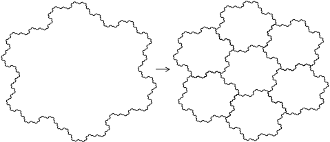
Figure 8. The subdivision of the tile type of the finite subdivision rule associated to the Lattès map with $(a,b,c,d)=(2,-3,1,2)$.

Next suppose that $(a,c)=(1,1)$. Figure 9 shows building blocks for this case. For example, suppose that $(a,b,c,d)=(1,-3,1,2)$ and $\beta=0$. The slope of the edge of $T$ containing $\psi(\beta)=0$ is negative, so we choose the fourth edge path in Figure 9. Since $\psi(\tau+\beta)=\psi(\tau)=\psi(b\alpha^{-1}+d\alpha^{-1}\tau)=\psi(-3\alpha^{-1}+2\alpha^{-1}\tau)$, the slope of the edge of $T$ containing $\psi(\tau+\beta)$ is positive, so we also choose the second edge path in Figure 9. We complete these two edge paths in the straightforward way to the fundamental domain shown in the left portion of Figure 10. For another example we take $(a,b,c,d)=(1,-6,1,2)$ and $\beta=0$. Since $\psi(\beta)=0$, the slope of the edge of $T$ containing $\psi(\beta)$ is negative, so we choose the fourth edge path in Figure 9. Since $\psi(\tau+\beta)=\psi(\tau)=\psi(-6\alpha^{-1}+2\alpha^{-1}\tau)$, the slope of the edge of $T$ containing $\psi(\tau+\beta)$ is negative, so we also choose the first edge path in Figure 9. One way to complete these two edge paths to a fundamental domain is shown in the right portion of Figure 10. Just as for the case in which $(a,c)=(2,1)$, whenever $(a,c)=(1,1)$ and the degree of $f$ is sufficiently large we obtain a fundamental domain which determines a finite subdivision rule whose mesh approaches 0 combinatorially.

Figure 9. Building blocks for constructing fundamental domains for the cases in which $(a,c)=(1,1)$.

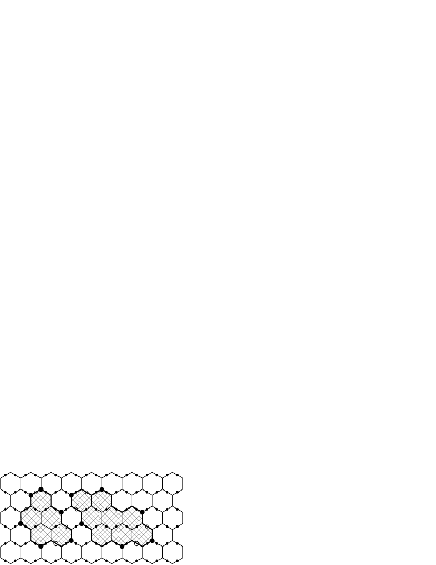
Figure 10. Fundamental domains for the cases in which $(a,b,c,d)=(1,-3,1,2)$ with $\beta=0$ and $(a,b,c,d)=(1,-6,1,2)$ with $\beta=0$.

Finally suppose that $(a,c)=(0,1)$. Figure 11 shows building blocks for this case. For example, suppose that $(a,b,c,d)=(0,-4,1,1)$ and $\beta=0$. The slope of the edge containing $\psi(\beta)=0$ is negative, so we choose the third edge path in Figure 11. Since $\psi(\tau+\beta)=\psi(\tau)=\psi(b\alpha^{-1}+d\alpha^{-1}\tau)=\psi(-4\alpha^{-1}+\alpha^{-1}\tau)$, the slope of the edge of $T$ containing $\psi(\tau+\beta)$ is positive, so we also choose the second edge path in Figure 11. We complete these two edge paths as shown in the left portion of Figure 12 to obtain a fundamental domain. For another example we take $(a,b,c,d)=(0,-7,1,0)$ and $\beta=1$. The slope of the edge containing $\psi(\beta)=\psi(1)=\psi(a\alpha^{-1}+c\alpha^{-1}\tau)=\psi(\alpha^{-1}\tau)$ is positive, so we choose the fourth edge path in Figure 11. Since $\psi(\tau+\beta)=\psi(\tau+1)=\psi((a+b)\alpha^{-1}+(c+d)\alpha^{-1}\tau)=\psi(-7\alpha^{-1}+\alpha^{-1}\tau)$, the slope of the edge of $T$ containing $\psi(\tau+\beta)$ is negative, so we choose the first edge path in Figure 11. We complete these two edge paths as shown in the right portion of Figure 12 to obtain a fundamental domain. As before whenever $(a,c)=(0,1)$ and the degree of $f$ is sufficiently large we obtain a fundamental domain which determines a finite subdivision rule whose mesh approaches 0 combinatorially.

Figure 11. Building blocks for constructing fundamental domains for the cases in which $(a,c)=(0,1)$.

Figure 12. Fundamental domains for the cases in which $(a,b,c,d)=(0,-4,1,1)$ with $\beta=0$ and $(a,b,c,d)=(0,-7,1,0)$ with $\beta=1$.

This completes the proof of Theorem 3.1.

∎

Theorem 3.10.

Every nonrigid Lattès map is the subdivision map of a finite subdivision rule with one tile type, and the tile has the form of type 1 in Figure 1.

Proof.

Let $f$ be a nonrigid Lattès map. Let $\widetilde{f}(z)=\alpha z+\beta$ be a lift of $f$. Then $\alpha\in\mathbb{Z}$, and we may assume that $\alpha\geq 2$. Let 1 and $\tau$ form a basis of the usual lattice $\Lambda$ with $\text{Im}(\tau)>0$. We may add any element of $2\Lambda$ to $\beta$, so we assume that $\beta\in\{0,1,\tau,1+\tau\}$.

Recall that Figure 1 shows five types of planar tilings. We construct a tiling $S^{\prime}$ of the plane with type 1 so that every tile of $S^{\prime}$ is a parallelogram. Furthermore one of the parallelograms of $S^{\prime}$ is chosen to be as in Figure 13. If $\beta=1$, then we choose the leftmost parallelogram. If $\beta=\tau$, then we choose the middle parallelogram. If $\beta=1+\tau$, then we choose the rightmost parallelogram. If $\beta=0$, then we choose any of these. Let $P$ denote the chosen parallelogram.

Figure 13. The parallelogram $P$.

The tiling $S^{\prime}$ is constructed so that $\beta$ is a vertex with valence 4. From this it follows that $F=\widetilde{f}(P)$ is a union of tiles of $S^{\prime}$. The parallelogram $P$ is really a hexagon because it has two vertices with valence 2. The two edges which contain one of the vertices with valence 2 are interchanged by a rotation of order 2. This pairs four of the six edges of $P$. The remaining two edges of $P$ are paired by a translation. In the same way $F$ has six edges which are paired so that $\widetilde{f}$ respects these edge pairings. As in the proof of Theorem 3.1, we obtain a finite subdivision rule $\mathcal{R}$ with one tile type. Not as in the proof of Theorem 3.1, in the present situation $f$ is already the subdivision map of $\mathcal{R}$.

This proves Theorem 3.10.

∎

Corollary 3.11.

Every map in almost every analytic conjugacy class of Lattès maps is the subdivision map of a finite subdivision rule with one tile type.

Proof.

This follows from Theorem 3.1, Theorem 3.10, and the last statement in Section 1, namely, that there are only finitely many analytic conjugacy classes of rigid Lattès maps with bounded degree.

∎

4. An exceptional quadratic Lattès map

This section deals with the Lattès map $f$ with lift $\widetilde{f}(z)=\alpha z$, where $\alpha=(1+\sqrt{-7})/2$ and the usual lattice $\Lambda$ is generated by 1 and $\alpha$. We prove that $f$ is not the subdivision map of a finite subdivision rule with one tile type, $f$ is not the subdivision map of a finite subdivision rule with two tile types and 1-skeleton of the subdivision complex homeomorphic to a circle, and $f$ is the subdivision map of a finite subdivision rule with two tile types.

The minimal quadratic equation satisfied by $\alpha$ is $\alpha^{2}-\alpha+2=0$. Since the constant term is $\alpha\overline{\alpha}=2$, the map $f$ is indeed quadratic. Moreover $\widetilde{f}(0)=0$, $\widetilde{f}(1)=\alpha$, $\widetilde{f}(\alpha)=\alpha^{2}\equiv\alpha\mod 2\Lambda$ and $\widetilde{f}(\alpha+1)=\alpha^{2}+\alpha\equiv 0\mod 2\Lambda$. Let $A=\wp(\alpha+1)$, $B=\wp(1)$, $X=\wp(0)$, and $Y=\wp(\alpha)$. Then $f(A)=X$, $f(B)=Y$, $f(X)=X$, and $f(Y)=Y$. Since $A$, $B$, $X$, and $Y$ are the only postcritical points of $f$, one critical point of $f$ maps to $A$ and one critical point of $f$ maps to $B$. We normalize so that $\infty$ and 0 are the critical points of $f$ with $f(\infty)=A$ and $f(0)=B$. Figure 14 shows the mapping scheme for $f$. Integers next to arrows are local mapping degrees.

We can normalize $f$ so that $f(z)=\frac{Az^{2}+B}{z^{2}+1}$. Since $X=f(X)=f(A)$, $Y=f(Y)=f(B)$, and $f$ is even, $X=-A$ and $Y=-B$. Hence $\frac{A^{3}+B}{A^{2}+1}=-A$ and $\frac{AB^{2}+B}{B^{2}+1}=-B$. This gives $B=-2A^{3}-A$ and $AB+1=-B^{2}-1$. Substituting $B=-A(2A^{2}+1)$ into the equation $AB+1=-B^{2}-1$ yields $0=2A^{6}+A^{4}+1=(A^{2}+1)(2A^{4}-A^{2}+1)$. If $A=\pm i$ then $B=A$, so $2A^{4}-A^{2}+1=0$. Hence $f(z)=\frac{Az^{2}+B}{z^{2}+1}$, where $A^{2}=\frac{1\pm\sqrt{-7}}{4}$ and $B=-A(2A^{2}+1)$. That is, either $2A^{2}=\alpha$ or $2A^{2}=\overline{\alpha}$. (By choosing $0$ and $\infty$ to be the fixed postcritical points, in [7, Section B.4] Milnor gives the alternate form $f(z)=z\frac{z+\alpha^{2}}{\alpha^{2}z+1}$ for $f$.)

Figure 14. The mapping scheme of $f$.

We first prove by contradiction that $f$ is not the subdivision map of a finite subdivision rule with one tile type. Suppose that $f$ is the subdivision map of a finite subdivision rule $\mathcal{R}$ with one tile type. Let $T$ be the 1-skeleton of the subdivision complex of $\mathcal{R}$. By Lemma 2.1, we may and do assume that the only vertices of $T$ with valence $1$ or $2$ are postcritical points.

Lemma 4.1.

No vertex of $T$ is a critical point of $f$.

Proof.

If a critical point of $f$ is a vertex of $T$, then it is an accidental vertex (not a postcritical point). A tree with type 1 or 2 has no accidental vertices. The postcritical vertices of trees of type 3 and 5 all have valence 1, and so a critical vertex would have valence at most 2, which is impossible. Suppose that $T$ has type 4. Then $T$ has just one accidental vertex, the vertex with valence 3. By symmetry we may assume that this vertex is $\infty$. As before since $\infty$ has valence greater than 2, $f(\infty)=A$ must have valence greater than 1. So $A$ is the vertex with valence 2. But then $f(A)$ also has valence at least 2 because the degree of $f$ at $A$ is 1. This is impossible. This shows that no vertex of $T$ is a critical point of $f$.

∎

Lemma 4.2.

Let $p$ and $q$ be distinct vertices of $T$ such that $f(p),f(q)\in\{p,q\}$. Then the open segment $(p,q)$ of $T$ contains a critical point.

Proof.

If $f$ maps both $p$ and $q$ to the same vertex, then because $f$ maps the segment $(p,q)$ into the tree $T$, the image of $(p,q)$ under $f$ must be folded somewhere. Such a fold is the image of a critical point. So $(p,q)$ contains a critical point in this case.

Now suppose that $f(p)=p$ and $f(q)=q$ and that $(p,q)$ contains no critical point of $f$. Then $f$ does not fold the segment $[p,q]$ anywhere. It follows that $f$ maps $[p,q]$ homeomorphically onto $[p,q]$. But then the edges in $[p,q]$ never subdivide. This implies that the mesh of our finite subdivision rule does not go to 0, contrary to the fact that $f$ is an expanding map. So the lemma holds if $f(p)=p$ and $f(q)=q$.

Finally, the case in which $f(p)=q$ and $f(q)=p$ can be proved just as in the case in which $f(p)=p$ and $f(q)=q$.

This proves Lemma 4.2.

∎

Lemma 4.3.

Neither $A$ nor $B$ is in the closed segment $[X,Y]$.

Proof.

Proceeding by contradiction, we may assume by symmetry that $A\in[X,Y]$. Since $f(A)=X$ and $f(Y)=Y$ there exists a point in $(A,Y)$ which maps to $A$. This point must be $\infty$. Since $f$ maps $A$ to $X$ with degree 1, $f([X,Y])$ contains a nontrivial segment which meets $[X,Y]$ at $X$. But then there exists a nontrivial segment $s$ in $T$ which contains a vertex of $T$ with valence 1 and has $s\cap[X,Y]=X$. This vertex with valence 1 must be $B$. Since $f(X)=X$ and $f(B)=Y$, it follows that $s$ contains a preimage of $A$, namely, $\infty\in s$. This is impossible.

∎

Now we apply Lemma 4.2 to see that there exists a critical point in $[X,Y]$. By symmetry we may assume that $\infty\in[X,Y]$. Lemma 4.3 shows that $A\notin[X,Y]$. Let $v$ be the vertex of $[X,Y]$ which is closest to $A$ in $T$. If $v=Y$, then because $f(X)=X$ and $f(\infty)=A$, $f$ maps some point in $(X,\infty)\subseteq(X,Y)$ to $Y$. This point must be $B$, which is impossible by Lemma 4.3. Hence $v\neq Y$. Likewise $v\neq X$. So $v$ is a vertex in $(X,Y)$ with valence at least 3.

In this paragraph we assume that $v$ is the only vertex of $T$ with valence at least 3. As in the previous paragraph we see that $v$ is the vertex in $[X,Y]$ which is closest to both $A$ and $B$. Lemma 4.1 implies that $v$ is not a critical point. Hence $f(v)$ has valence at least 3, and so $f(v)=v$. Since $f(X)=X$ and $f(v)=v$, Lemma 4.2 implies that $(X,v)$ contains a critical point $p$. Since the critical point maps to $A$ or $B$, $(X,v)$ contains a preimage of $v$. Likewise $(v,Y)$ contains a critical point $q$, and $(q,Y)$ contains a preimage of $v$. We now have three points mapping to $v$, which is impossible.

To complete this argument we assume that $T$ contains two vertices $u$ and $v$ with valence 3, that one of them, $v$, is in $(X,Y)$, and that either $u\in(X,Y)$ or $v$ is the vertex in $[X,Y]$ closest to $u$. As in the previous paragraph, we see that $f(u),f(v)\in\{u,v\}$. First suppose that $f(u)=u$ and $f(v)=v$. Lemma 4.2 implies that $(u,v)$ contains a critical point. So does the segment from $X$ to $[u,v]$ as well as the segment from $Y$ to $[u,v]$. This is impossible. Next suppose that $f(u)=v$ and $f(v)=u$. Let $w\in(u,v)$. Then $(u,v)$ contains a preimage of $w$. So does the segment from $X$ to $[u,v]$ as well as the segment from $Y$ to $[u,v]$. We now have three preimages of $w$, which is impossible. We are left with the case in which $f(u)=f(v)\in\{u,v\}$. Suppose in addition that $u\notin[X,Y]$. Recall that $\infty$ is a critical point in $[X,Y]$. Choose $z\in\{X,Y\}$ so that $v\notin[z,\infty]$. Then the image of $[z,\infty]$ covers $[u,v]$, and so $[z,\infty]$ contains a preimage of $f(u)=f(v)$, giving three preimages, which is impossible. So $u\in[X,Y]$. Now choose $z\in\{X,Y\}$ so that neither $u$ nor $v$ lies in $(z,f(v))$. Lemma 4.2 implies that $(z,f(v))$ contains a critical point $p$. But then $(z,p)$ contains a preimage of $f(v)$, giving a third preimage of $f(v)$, which is once more impossible.

The proof that $f$ is not given by a finite subdivision rule with one tile type is now complete.

We next prove by contradiction that $f$ is not given by a finite subdivision rule with two tile types with 1-skeleton of the subdivision complex homeomorphic to a circle. Suppose that $f$ is given by a finite subdivision rule with two tile types with 1-skeleton $G$ of the subdivision complex homeomorphic to a circle. If some open edge of $G$ is not in $f(G)$, then we delete that open edge to obtain a finite subdivision rule for $f$ with one tile type. Since such a finite subdivision rule does not exist, it follows that $f(G)=G$.

In this paragraph we assume that the restriction of $f$ to $G$ is locally injective. Then the restriction of $f$ to $G$ is a covering map with degree either 1 or 2. If this degree is 2, then every point in $G$ has two preimages, but both $A$ and $B$ have at most one preimage in $G$. If this degree is 1, then the restriction of $f$ to $G$ is a homeomorphism. In this case the edges of $G$ do not subdivide and the mesh of our finite subdivision rule fails to go to 0. So the restriction of $f$ to $G$ is not locally injective.

Since the restriction of $f$ to $G$ is not locally injective, $G$ contains a critical point. We may thus assume that $f$ is not locally injective at $\infty\in G$. Let $e_{1}$ and $e_{2}$ be the edges of $G$ which contain $A$ and suppose that $e_{1}$ is doubly covered by $f$ near $\infty$. But then $e_{2}$ is not in $f(G)$, for if it is, then some point other than $\infty$ maps to $A$, which is not the case. Thus $f$ is not given by a finite subdivision rule with two tile types with 1-skeleton homeomorphic to a circle.

We finally prove that $f$ is the subdivision map of a finite subdivision rule with two tile types. The left portion of Figure 15 shows a parallelogram which is a fundamental domain $F$ for the orbifold fundamental group $\Gamma$ of $f$. In addition to the vertices at the corners of $F$, there are vertices at 1 and $\alpha$. There is also an extra edge joining 0 and $\alpha$. The hatched region in the right portion of Figure 15 shows $\widetilde{f}^{-1}(F)$. To verify this it is useful to note that $\alpha^{2}-\alpha+2=0$ implies that $\alpha(1-\alpha)=2$ and so $1-\alpha=2\alpha^{-1}$. The last identity shows that $2\alpha^{-1}$ is drawn correctly. Moreover the fact that 0, 2 and $\alpha+1$ are vertices of the parallelogram $F$ implies that 0, $2\alpha^{-1}$ and $\alpha^{-1}+1$ are vertices of the parallelogram $\widetilde{f}^{-1}(F)$. Thus $\widetilde{f}^{-1}(F)$ is drawn correctly. Let $T$ be the tiling of the plane by the images of $F$ under $\Gamma$. Figure 16 shows a part of $T$ drawn with dashed line segments and part of $\widetilde{f}^{-1}(T)$ drawn with solid line segments. Few dashed line segments of $T$ are visible because most of them are obscured by the line segments of $\widetilde{f}^{-1}(T)$. Now it is clear that there exists a $\Gamma$-equivariant isotopy from $T$ to $\widetilde{f}^{-1}(T)$ rel $\Lambda$. This determines a finite subdivision rule $\mathcal{R}$ with two tile types, one triangle and one pentagon. Figure 17 gives a schematic description of the subdivisions of the tile types of $\mathcal{R}$. The edges drawn with dashes in Figure 17 are the edges whose edge types correspond to the line segments drawn with dashes in Figure 16. One easily checks that $\mathcal{R}$ has bounded valence and mesh approaching 0 combinatorially. It now follows as in the proof of the main theorem of [4] that $f$ is the subdivision map of a finite subdivision rule isomorphic to $\mathcal{R}$. A stereographic projection of the subdivision complex for $f$ is shown in Figure 18 with hats indicating images of 0, 1, $\alpha$, and $\alpha+1$.

Figure 15. The fundamental fundamental domain $F$ and $\widetilde{f}^{-1}(F)$.

Figure 16. A small part of the tiling $T$ and $\widetilde{f}^{-1}(T)$.

Figure 17. The finite subdivision rule $\mathcal{R}$.

Figure 18. The subdivision complex for $f$.

References

- [1] M. Bonk and D. Meyer, Markov partition of expanding Thurston maps, in preparation.
- [2] Z. I. Borevich and I. R. Shafarevich, Number Theory, Academic Press, New York and London, 1966.
- [3] J. W. Cannon, W. J. Floyd and W. R. Parry, Expansion complexes for finite subdivision rules I, Conform. Geom. Dyn. 10 (2006), 63–99.
- [4] J. W. Cannon, W. J. Floyd and W. R. Parry, Constructing subdivision rules from rational maps, Conform. Geom. Dyn. 11 (2007), 128–136.
- [5] J. W. Cannon, W. J. Floyd, W. R. Parry, and K. M. Pilgrim, Subdivision rules and virtual endomorphisms, Geom. Dedicata 141 (2009), 181–195.
- [6] A. Douady and J. H. Hubbard, A proof of Thurston’s topological characterization of rational functions, Acta Math. 171 (1993), 263–297.
- [7] J. Milnor, Pasting together Julia sets: a worked out example of mating, Experimental Math. 13 (2004), 55–92.