Foreground influence on primordial non-Gaussianity estimates: needlet analysis of WMAP 5-year data

Abstract

We constrain the amplitude of primordial non-Gaussianity in the CMB data taking into account the presence of foreground residuals in the maps. We generalise the needlet bispectrum estimator marginalizing over the amplitudes of thermal dust, free-free and synchrotron templates. We apply our procedure to WMAP 5 year data, finding $f_{\rm NL}=38\pm 47$ (1 $\sigma$), while the analysis without marginalization provides $f_{\rm NL}=35\pm 42$. Splitting the marginalization over each foreground separately, we found that the estimates of $f_{\rm NL}$ are positively cross correlated of $17\%,12\%$ with the dust and synchrotron respectively, while a negative cross correlation of about $-10\%$ is found for the free-free component.

1 Introduction

There has been considerable activity recently in constraining the amount of non-Gaussianity present in CMB data. This is principally motivated by theoretical interest into deviations of primordial fluctuations from Gaussian statistics— a natural outcome of several implementations of the inflationary scenario, which can be used as a tool to rule out specific models. More mundanely, non-Gaussianity can also be produced by undetected systematics, which may suggest problems in the dataset. It could also indicate that elements are missing in the standard cosmological model; for example, anomalies which have recently been detected on large scales have been put forward as evidence of cosmic defects or an anisotropic universe.

The primordial non-Gaussianity in inflationary models is usually characterised through the introduction of the $f_{\rm NL}$ parameter (see e. g.  Luo (1994); Heavens (1998); Spergel & Goldberg (1999); Komatsu & Spergel (2001)) which sets the amplitude of the non-linear contribution with respect to the leading order:

$$\Phi({\bf x})=\Phi_{\rm L}({\bf x})+f_{\rm NL}(\Phi_{\rm L}({\bf x})^{2}-\langle\Phi_{\rm L}({\bf x})^{2}\rangle)$$ (1)

where $\Phi({\bf x})$ is the primordial gravitational potential and $\Phi_{\rm L}({\bf x})$ is a Gaussian field. In the following we will focus on primordial non-Gaussianity of local type described by Eq. 1. Different inflationary scenarios predict different values of $f_{\rm NL}$; while in the standard slow roll inflationary scenario (Guth, 1981; Sato, 1981; Linde, 1982; Albrecht & Steinhardt, 1982), $f_{\rm NL}$ it is predicted to be of the order of unity (see also (Maldacena, 2003; Acquaviva et al., 2003)), in several alternative models (Lyth & Wands, 2002; Linde & Mukhanov, 2006; Alabidi & Lyth, 2006; Mizuno et al., 2008; Khoury, 2002; Steinhardt & Turok, 2002; Lehners & Steinhardt, 2008) it can take much larger values (see e.g. Bartolo et al. (2004) for a review). Since the release of the first year WMAP data (Bennett et al., 2003; Komatsu et al., 2003), there has been a drastic reduction of the upper limits of $f_{\rm NL}$. The most recent constraints coming from WMAP data using different techniques can be found in Komatsu et al. (2009), Smith et al. (2009), Yadav & Wandelt (2008), Curto et al. (2009), Curto et al. (2009), Pietrobon et al. (2009), Rudjord et al. (2009), Rudjord et al. (2009), Smidt et al. (2009) and Vielva & Sanz (2009). Results on $f_{\rm NL}$ with suborbital experiments can be found in (Natoli et al., 2009; Curto et al., 2008). Interestingly, some of these (Yadav & Wandelt, 2008; Rudjord et al., 2009) reported a non-null detection of $f_{\rm NL}$ at more than 2$\sigma$ level in the WMAP data, leading to a debate on the significance of the signal and whether it may have a cosmological origin or be due to residual foreground or instrumental contamination (Smith et al., 2009).

Non-Gaussianity is also expected from unremoved contamination from astrophysical sources, or foregrounds. When component separation techniques are applied to CMB data (e.g. Maino et al. (2002); Tegmark et al. (2003); Bonaldi et al. (2007); Leach et al. (2008); Bernui & Rebouças (2009)), residual foregrounds remain, and while they are subdominant, they can still be a source of non-Gaussianity, and this could be confused with a primordial signature and affect the constraints on $f_{\rm NL}$.

In this paper, which is complementary to our previous work (Pietrobon et al., 2009), we aim at generalising the needlet bispectrum estimator to the case in which such foreground residuals are present in the data. Another marginalization technique, using the fast cubic estimator on the bispectrum data, can be found in Smith et al. (2009).

The paper is organised as follows. In section 2 we give a brief introduction of the needlets and their bispectrum; section 3 addresses the generalisation of the needlet bispectrum estimator in presence of foreground residuals, in section 4 we describe the CMB and the foregrounds dataset used and show our results, in Section 5 we comment on our findings.

2 Needlet formalism and general applications

Here we give a brief summary of the needlet formalism, but one should refer to Marinucci et al. (2008) and references therein for a more complete discussion. The mathematical approach is described in Narcowich et al. (2006), Baldi et al. (2006), Baldi et al. (2007) and Baldi et al. (2008).

Needlets are filter functions with some appealing properties; in particular they are well localised both in real and harmonic space, and are straight forward to implement in practice. The analytical function describing a needlet is:

$$\psi_{jk}(\hat{\gamma})=\sqrt{\lambda_{jk}}\sum_{\ell}b\Big{(}\frac{\ell}{B^{j}}\Big{)}\sum_{m=-\ell}^{\ell}\overline{Y}_{\ell m}(\hat{\gamma})Y_{\ell m}(\xi_{jk}).$$ (2)

Here, $\hat{\gamma}$ is the direction of a given point on the sphere, $\{\xi_{jk}\}$ are the cubature points, weighted by $\lambda_{jk}$, for a given spatial frequency $j$ and location $k$ and $b(\cdot)$ is a filter function defined in harmonic space. $B$ is a free parameter which, once fixed, determines the width of $b(\cdot)$ and determines the range of multipoles which appears in Eq. 2. Its value is set according to the angular scales one is interested in exploring. It can be shown (see Marinucci et al. (2008)) that assuming certain properties of the function $b(\cdot)$ (e.g. finite support in $\ell$-space and smoothness), the needlets are quasi-exponentially localised around the $\hat{\gamma}$ direction (Narcowich et al., 2006). These properties allow needlets to be used as a scale dependent analyser in both the harmonic and pixel domains. For the reader interested in the details of a practical implementation of needlets using Healpix package (Górski et al., 2005), we refer to Pietrobon et al. (2006). From the operational point of view, the quantities of interest are the coefficients of the expansion on the needlets basis defined as:

$$\beta_{jk} = \int_{S^{2}}T(\hat{\gamma})\psi_{jk}(\hat{\gamma})d\Omega$$ (3)

$$= \sqrt{\lambda_{jk}}\sum_{\ell}b\Big{(}\frac{\ell}{B^{j}}\Big{)}\sum_{m=-\ell}^{\ell}a_{\ell m}Y_{\ell m}(\xi_{jk}).$$

These coefficients can be used for reconstructing a map as:

$$T(\hat{\gamma})\equiv\sum_{j,k}\beta_{jk}\psi_{jk}(\hat{\gamma})$$ (4)

As with other varieties of wavelets, needlets allow a multi-scale analysis, which is useful for many kinds of data analyses, such as denoising (Sanz et al. (1999)), point source extraction (see for instance, Cayón et al. (2000); Vielva et al. (2003)), asymmetry studies (Cruz et al., 2007; Pietrobon et al., 2008; McEwen et al., 2008; Vielva et al., 2007; McEwen et al., 2008) and for cross correlating different datasets, as for example CMB and large scale surveys for the detection of the Integrated Sachs-Wolfe effect, which sets constraints on dark energy (Pietrobon et al., 2006; Vielva et al., 2006). From the coefficients of Eq. 3 we can estimate the binned CMB power spectrum:

$$\beta_{j}\equiv\sum_{jk}\beta_{jk}^{2}=\sum_{\ell}b_{\ell,j}^{2}\frac{2\ell+1}{4\pi}\mathcal{C}_{\ell}$$ (5)

(see Faÿ et al. (2008) and Pietrobon et al. (2006, 2008) for an application to real data). It is straightforward to generalise this formalism to higher order statistics like the needlet bispectrum (Lan & Marinucci, 2008; Pietrobon et al., 2009; Rudjord et al., 2009; Pietrobon et al., 2009; Rudjord et al., 2009):

$$S_{j_{1}j_{2}j_{3}}=\frac{1}{\tilde{N}_{\rm p}}\sum_{\rm k}\frac{\beta_{j_{1}k}\beta_{j_{2}k}\beta_{j_{3}k}}{\sigma_{j_{1}}\sigma_{j_{2}}\sigma_{j_{3}}}.$$ (6)

Here $k$ spans over the pixels of the region of interest, $N_{p}$ is the total number of these pixels and $\sigma_{j}$ is the standard deviation of the needlet coefficients. Eq. 6 has been applied to constrain $f_{\rm NL}$ with a needlet analysis, since it has been proven to be proportional to the reduced bispectrum (Komatsu & Spergel, 2001), and thus to the non-linear parameter $f_{\rm NL}$ (Pietrobon et al., 2009; Rudjord et al., 2009; Pietrobon et al., 2009; Rudjord et al., 2009):

$$S_{j_{1}j_{2}j_{3}}\propto f_{\rm NL}\sum_{k}(\beta^{\rm NG}_{j1k}\beta^{G}_{j2k}\beta^{G}_{j3k}+\rm{perms}).$$ (7)

The needlets bispectrum has several useful properties. It can be shown that, given the localisation properties of needlets, their bispectrum is not heavily affected by the correlation introduced by the masking procedure. Another advantage is that there is no need to calculate Wigner coefficients (as a pure bispectrum analysis requires), which is a time consuming step, especially when high multipoles are considered. These properties translate into a good detection power in constraining primordial non-Gaussianity (see (Pietrobon et al., 2009; Rudjord et al., 2009; Rudjord et al., 2009)) comparable with the fast cubic estimator introduced by Komatsu et al. (2005) and applied in Komatsu et al. (2009) and Yadav & Wandelt (2008).

3 Method

In this section we generalise the $f_{\rm NL}$ estimator from the needlet bispectrum (Pietrobon et al., 2009) in presence of residual foregrounds.

When constraining primordial non-Gaussianity, one can estimate $f_{\rm NL}$ by minimising the chi-square:

$$\chi^{2}(f_{\rm NL})=Y^{T}\mathbf{C}^{-1}Y,$$ (8)

where $Y=Y^{obs}-\langle Y(f_{\rm NL})\rangle$ is the difference between an ordered array of data ($Y^{obs}$) and the corresponding theoretical prediction $Y(f_{\rm NL})$. The data can take many forms, such as, the values of Minkowski functionals for different thresholds (Hikage et al., 2006), the densities of valleys or hills when using the local curvature (Cabella et al., 2005) or, as in this case, the values of the needlet bispectrum (Pietrobon et al., 2009; Rudjord et al., 2009; Rudjord et al., 2009). In the presence of the expected weak non-Gaussianity, the covariance matrix $C$ can be calculated via Gaussian simulations with the same power spectrum as the observed data.

It has been shown (Pietrobon et al., 2009; Rudjord et al., 2009) that an unbiased estimator for $f_{\rm NL}$ is given by

$$f_{\rm NL}=\frac{\sum_{\mu\mu^{\prime}}S^{\rm obs}_{\mu}\mathbf{C}^{-1}_{\mu\mu^{\prime}}S^{\rm th}_{\mu^{\prime}}}{\sum_{\mu\mu^{\prime}}S^{\rm th}_{\mu}\mathbf{C}^{-1}_{\mu\mu^{\prime}}S^{\rm th}_{\mu^{\prime}}},$$ (9)

where $\mu$ runs over the triplets $\{j_{1}j_{2}j_{3}\}$ and $S^{\rm th}_{\mu}$ represents the ensemble average of primordial non-Gaussian realisations ($f_{\rm NL}=1)$. Although the process of foreground reduction could make things more complicated, we can make the minimal assumption that the final map, contaminated by foreground residuals, can be modeled as:

$$T^{\rm sim}(\hat{\gamma}) = T^{\rm G}(\hat{\gamma})+f_{\rm NL}T^{\rm NG}(\hat{\gamma})+N(\hat{\gamma})$$ (10)

$$+ \alpha_{\rm D}\,D(\hat{\gamma})+\alpha_{\rm F}\,F(\hat{\gamma})+\alpha_{\rm S}\,S(\hat{\gamma}),$$

where $D$, $F$ and $S$ are the thermal dust, free-free emission and synchrotron radiation maps, respectively and the noise map $N$ is assumed to be Gaussian. Calculating the needlets coefficients from Eq. 10 we obtain

$$\beta_{jk}=\beta_{jk}^{\rm G}+\beta_{jk}^{\rm N}+f_{\rm NL}\beta_{jk}^{\rm NG}+\alpha_{\rm D}\beta_{jk}^{\rm D}+\alpha_{\rm F}\beta_{jk}^{\rm F}+\alpha_{\rm S}\beta_{jk}^{\rm S}.$$ (11)

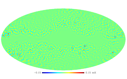
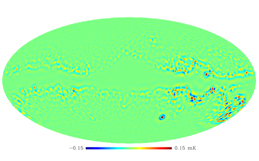
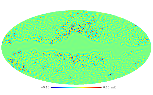
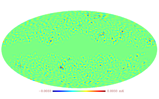
In Figure 1 we show the needlet coefficients in the case of $B=2$ and $j=6$ for the three foregrounds templates – dust, free-free and synchrotron – once they have been masked. The maps were converted in thermodynamic temperature for each channel and combined to form one single map. Each template was divided by a factor 10, which is the level of residuals expected. This factor was estimated in harmonic space through a Monte Carlo Markov Chain algorithm. The foreground reduced map used in this analysis has been produced by optimally combining the W, V and Q WMAP bands as described below (Eq. 17.)

Figure 1: The needlets coefficients with $B=2$ and $j=6$, which are sensitive to $64<\ell<127$, or angular scales of a few degrees. The maps shown are for thermal dust (top), free-free, synchrotron and the assumed primordial non-Gaussian signal for $f_{\rm NL}=50$ (bottom). The Kq$75$ mask has been applied.

The angular power spectrum of this optimal CMB map has been compared to a linear combination of synchrotron, free-free, Galactic dust, CMB and noise. Synchrotron, free-free and Galactic dust maps are estimated from the data using exactly the same combination in Eq. 17, while CMB and noise are estimated through simulations for each band and then combined in the same way as data. 100 realisations of CMB maps have then been generated in order to take into account the uncertainty due to the cosmic variance. 100 realisations of noise have been created with variance consistent with the data and then fitted the amplitude coefficients $p_{\gamma}$ of each component $\gamma$, such that

$$\mathcal{C}_{\ell}^{tot}=\mathcal{C}_{\ell}^{\rm CMB}+\sum_{\gamma}p_{\gamma}\mathcal{C}_{\ell}^{\gamma}+N_{\ell},$$ (12)

where $N_{\ell}$ is the detector noise (a similar procedure has been applied in Veneziani et al. (2009)). We find $p_{\rm synch}<0.1\times 10^{-1}$, $p_{\rm dust}<1.0\times 10^{-1}$ and $p_{\rm ff}<0.6\times 10^{-1}$. The coefficients $p_{\rm\gamma}$ provide an indication of the power spectrum contamination percentage by the foreground residuals. The effect on the bispectrum is estimated to be of the order of $\sim 10^{-3}$.

We can compute the needlet bispectrum expected from the model of the model of residuals described in Eq. 10, by substituting Eq. 11 into the definition of the bispectrum. In principle, this will include many terms including triple products of the various contributions. On average, the product of the Gaussian contributions should be zero, and the lowest order contribution from the primordial non-Gaussianity is that shown in Eq. 7. We also expect on average that cross terms like $\beta^{\rm NG}\beta^{\rm I_{1}}\beta^{\rm I_{2}}$ (I=$\{$D,F,S$\}$ will also be zero, as the foregrounds should be uncorrelated with the primordial signal.

However, cross terms which include different foregrounds, of the form $\beta^{\rm I_{1}}\beta^{\rm I_{2}}\beta^{\rm I_{3}}$, could potentially be non-zero, particularly if there are physical reasons to expect correlations. (For example, both synchrotron and free-free are sensitive to the free electron density.) Even if such terms are zero on average, they will not be zero for specific realisations of the foregrounds; indeed if we think we know the foreground templates, we can calculate these terms directly. For simplicity here, we ignore such terms and focus only on the ’auto-bispectra.’ This has the advantage that solving for the best fit amplitudes involves solving a simple set of linear equations. (Cross terms make the equations non-linear, requiring a numerical solution.)

With this assumption, the theoretical needlet bispectrum ($S$) in presence of foreground residuals can be written as:

$$S_{j_{1}j_{2}j_{3}}=f_{\rm NL}S^{\rm NG}_{j_{1}j_{2}j_{3}}+A_{D}S^{\rm D}_{j_{1}j_{2}j_{3}}+A_{F}S^{\rm F}_{j_{1}j_{2}j_{3}}+A_{S}S^{\rm S}_{j_{1}j_{2}j_{3}},$$ (13)

where

$$S^{\rm NG}_{j_{1}j_{2}j_{3}}=\sum_{k}\frac{\beta_{j_{1}k}^{\rm G}\beta_{j_{2}k}^{\rm G}\beta_{j_{3}k}^{\rm NG}}{\sigma_{j_{1}}\sigma_{j_{2}}\sigma_{j_{3}}}+{\rm perms};$$

$$S^{\rm I}_{j_{1}j_{2}j_{3}}=\sum_{k}\frac{\beta_{j_{1}k}^{\rm I}\beta_{j_{2}k}^{\rm I}\beta_{j_{3}k}^{\rm I}}{\sigma_{j_{1}}\sigma_{j_{2}}\sigma_{j_{3}}}.$$ (14)

For ease of notation, we have defined the foreground amplitudes as $A_{\rm I}=\alpha^{3}_{\rm I}.$

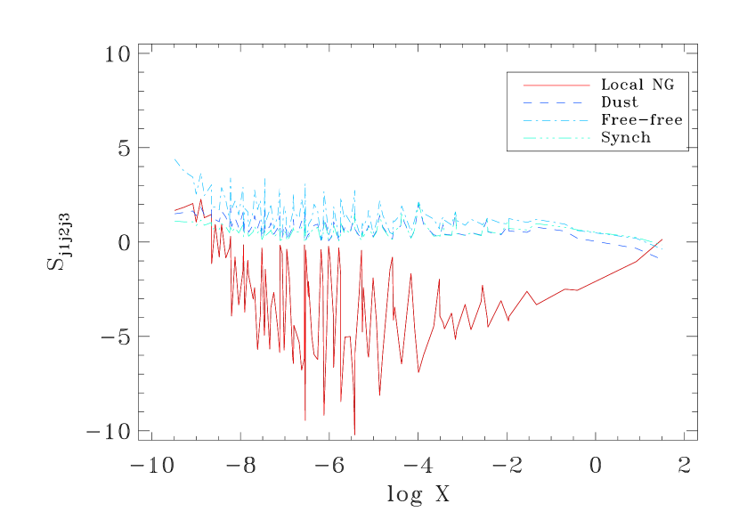
In Figure 2 we show the bispectrum for the primordial non-Gaussianity with $f_{\rm NL}=50$ and for the foreground templates of WMAP data normalised according to the prescription discussed previously. The bispectrum is shown as a function of the quantity $X=1/j_{1}j_{2}+1/j_{1}j_{3}+1/j_{3}j_{2}$, which orders them roughly according to their variance (as can be seen in Figure 3.)

Figure 2: Bispectrum amplitudes for the primordial non-Gaussian signal ($f_{\rm NL}=50$), and the three WMAP data foreground templates suppressed by a factor 1000, roughly corresponding to the expected signal of the residual foregrounds.

The $\chi^{2}$ expression (Eq. 8) can be easily generalised as follows:

$$\chi^{2} = \big{(}S^{obs}_{\mu}-S_{\mu}(f_{\rm NL})-S^{i}_{\mu}(A_{i})\big{)}C_{\mu\mu^{\prime}}^{-1}$$ (15)

$$\big{(}S^{obs}_{\mu^{\prime}}-S_{\mu^{\prime}}(f_{\rm NL})-S^{i}_{\mu^{\prime}}(A_{i})\big{)}^{T},$$

where $i$ refers to the i-th foreground template with the Einstein summation convention assumed, and $S^{i}_{\mu}$ is the needlet bispectrum of the given foreground. Minimising Eq. 15 with respect to $x=(f_{\rm NL},A_{\rm D},A_{\rm F},A_{\rm S})$ we obtain:

$$f_{\rm NL}=\frac{S_{i}^{\rm NG}C_{ij}^{-1}S_{j}^{obs}}{S_{i}^{\rm NG}C_{ij}^{-1}S_{j}^{\rm NG}}-\sum_{K}\frac{S_{i}^{\rm NG}C_{ij}^{-1}S_{j}^{\rm K}}{S_{i}^{\rm NG}C_{ij}^{-1}S_{j}^{\rm NG}}A_{\rm K}$$

$$A_{\rm I}=\frac{S_{i}^{\rm I}C_{ij}^{-1}S_{j}^{obs}}{S_{i}^{\rm I}C_{ij}^{-1}S_{j}^{\rm I}}-\sum_{K}\frac{S_{i}^{\rm I}C_{ij}^{-1}S_{j}^{\rm K}}{S_{i}^{\rm I}C_{ij}^{-1}S_{j}^{\rm I}}A_{\rm K}$$ (16)

where in each case the sum implicitly goes over the other signals $K=\{\rm NG,D,F,\rm S\}$.

The solution of the previous system provides us with the estimates of $f_{\rm NL}$ with the needlet bispectrum in presence of foreground residuals. In the following we present data and simulations where this estimator has been applied.

4 Data set, simulations and results

In the following, the needlets of the simulations and data will be calculated for B=2 unless specified otherwise. We used the publicly available WMAP 5-year data (Hinshaw et al., 2009). The CMB map has been obtained combining the foreground reduced maps for the channel Q,V,W according to:

$$T^{\rm obs}(\hat{\gamma})=\sum_{\rm ch}\frac{{n_{\rm obs}(\hat{\gamma})}}{\sigma^{2}_{ch}}T^{\rm red}_{\rm ch}(\hat{\gamma}),$$ (17)

where $n_{\rm obs}(\hat{\gamma})$ is the number of hits for a given point on the sphere $(\hat{\gamma})$, $\sigma_{ch}$ is the nominal sensitivity for the relative channel $ch$ and the superscript $red$ denotes the reduced dataset. We considered the WMAP data templates of dust, free-free and synchrotron emission at the resolution of $N_{\rm side}=256$ corrected by the conversion factors from antenna to thermodynamic temperature of the respective channel; we then combined them as in Eq. 17 to have one single map for each template. The data and foreground templates were then masked with Kq$75$ mask (downgraded to the same resolution as well) which covers the dominant Galactic emission over roughly the $30\%$ of the sky. We obtained our final constraints on $f_{\rm NL}$ by applying the estimator in its improved fashion to the WMAP 5-year data where:

• the covariance matrix $\mathbf{C}^{-1}$ was calibrated over 20,000 Gaussian simulations;

• the needlet foreground bispectra $S_{\rm D},S_{\rm F},S_{\rm S}$ were calculated on the templates described above;

• the primordial needlet bispectrum $S^{\rm NG}$ was calculated using over 100 primordial non-Gaussian maps (Liguori et al., 2007) convolved with the beams and combined as done for the Gaussian simulations (see also Elsner & Wandelt (2009) for an alternative algorithm to generate temperature and polarization primordial non Gaussian maps).

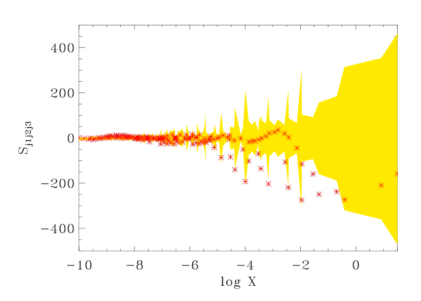
Figure 3 shows the data we used together with the average and the standard deviation derived from simulations. The error bars on $f_{\rm NL}$ were computed through the distribution of its estimates for 20,000 Gaussian realizations.

Figure 3: Needlets bispectrum measured from the WMAP 5-year temperature map. The shaded region marks the 68% confidence level computed from 20,000 Gaussian realisations.

In Figure 4 we show our results, where in each panel we show the estimate of $f_{\rm NL}$ with and without marginalizing over the foreground templates. Without marginalizing, we found $f_{\rm NL}=38\pm 42,85$ at 1$\sigma$ and 2$\sigma$, respectively. The marginalization over all the foregrounds brings the constraint to $f_{\rm NL}=41\pm 47,95$ with an increase of the error bars of about $10\%$ and a positive shift of the mean value. Although the larger error bars mean that we should not attach too much significance to the higher $f_{\rm NL}$ value, it would be interesting to investigate whether this could partially explain some positive detection present in literature (e. g.  Yadav & Wandelt (2008); Rudjord et al. (2009)). Further information can be obtained by looking at the estimates of $f_{\rm NL}$ marginalizing over the three foregrounds separately. The enlargement of the error bars due to each foreground is of the same order of magnitude, but the shift of the estimate seems to be mostly due to the dust component.

Figure 4: One dimensional likelihoods for the $f_{\rm NL}$ parameter. Solid lines represent marginalized likelihoods, whereas the dashed ones refer to the slice $A_{\rm foreg}=0$. The top left panel shows the analysis including all the three foregrounds, while the others are derived when a single foreground — dust (top right), free-free (bottom left) and synchrotron (bottom right) emission – is allowed to vary.

As a further check we carried out a Fisher analysis. (For a quick-start guide to Fisher matrix see Coe (2009).) So far we applied a Monte Carlo approach to find a good estimate of $f_{\rm NL}$ in presence of foreground contamination and quantify the scatter around this evaluation.

If the likelihood is close to Gaussian, the scatter can be well approximated by the Fisher approach, as the Cramer-Rao bound $\sigma_{\theta}\geq 1/(F^{-1})^{1/2}_{ii}$ becomes close to an equality. The Fisher matrix is defined as:

$$F_{ab}=\sum_{\rm\mu\mu^{\prime}}\frac{\partial S_{\rm\mu}^{\rm T}}{\partial a}C_{\rm\mu\mu^{\prime}}^{-1}\frac{\partial S^{\rm T}_{\rm\mu^{\prime}}}{\partial b}$$ (18)

where $S$ is the signal described in Eq. 13 and $\rm\mu$, $\rm\mu^{\prime}$, $a$ and $b$ run over the triplets $\{j_{1},j_{2},j_{3}\}$ and the parameter set $\{f_{\rm NL},A_{\rm D},A_{\rm F},A_{\rm S}\}$. In detail we have:

$$F=\tiny{\left(\begin{array}[]{cccc}S^{NG}C^{-1}S^{NG}&S^{NG}C^{-1}S^{\rm{D}}&S^{NG}C^{-1}S^{\rm{F}}&S^{NG}C^{-1}S^{\rm{S}}\\ S^{\rm D}C^{-1}S^{NG}&S^{\rm D}C^{-1}S^{\rm{D}}&S^{\rm D}C^{-1}S^{\rm{F}}&S^{\rm D}C^{-1}S^{\rm{S}}\\ S^{\rm{F}}C^{-1}S^{NG}&S^{\rm F}C^{-1}S^{\rm{D}}&S^{\rm F}C^{-1}S^{\rm{F}}&S^{\rm F}C^{-1}S^{\rm{S}}\\ S^{\rm{S}}C^{-1}S^{NG}&S^{\rm S}C^{-1}S^{\rm{D}}&S^{\rm S}C^{-1}S^{\rm{F}}&S^{\rm S}C^{-1}S^{\rm{S}}\\ \end{array}\right)}$$

where the sum over the triplets is implicit.

The marginalized error on $f_{\rm NL}$ arising from this Fisher analysis is $\Delta f_{\rm NL}=45$, very close to the limits obtained with the Monte Carlo approach; this confirms the efficiency of our estimation method. In Fig. 5 we show the 1$\sigma$ and 2$\sigma$ Fisher error ellipses together with the Markov chain output; here each plot presents the significance region in the case where the other parameters are fixed at their fiducial value. It can be seen that the free-free component seems slightly anti-correlated with $f_{\rm NL}$, the cross-correlation coefficient being $\rho\equiv\mathbf{-}S^{NG}C^{-1}S^{\rm{F}}/({S^{NG}C^{-1}S^{NG}\times S^{\rm F}C^{-1}S^{\rm{F}}})^{1/2}=-0.10$. The other foreground components, i.e. dust and synchrotron, show a positive correlation, demonstrated by the orientation of the ellipses, with $\rho=0.17$ and $\rho=0.12$, respectively. We can also calculate the cross-correlation between the various foreground amplitudes based on their non-Gaussianity: the dust-synchrotron correlation is $\rho=-0.87$, the dust-free-free correlation is $\rho=-0.29$ and the synchrotron-free-free correlation is $\rho=-0.58$. The scatter of the over-plotted distribution of Gaussian simulations on the same $A_{\rm I}$-$f_{\rm NL}$ plane is in excellent agreement with the ellipses, which confirms again the consistency of our procedure. We can also use the scatter in the foreground amplitudes to estimate limits on the foreground contamination using the bispectra; these are generally the same order as the limits arising from the fitting of the power spectrum discussed above.

As a check of our assumption that we are not strongly affected by potential cross-correlations among the foregrounds templates, we also considered the three foreground signals combined in a single foreground template. This effectively maps to a perfect covariance between the various foreground amplitudes. The analysis for this combination template is identical to the individual foreground analyses discussed above. We use $A_{\rm g}$ to describe the amplitude of the the needlet bispectrum of the total foreground map, obtained summing the three templates. We found $f_{\rm NL}=37\pm 43$ at 1 $\sigma$ confidence level, very close to the result when the foregrounds are included individually and assumed to be uncorrelated. We also plot the two-dimension scatter plot in the plane $f_{\rm NL}$-$A_{\rm g}$ in Fig. 5. The correlation results $\rho\simeq 0.14$, in good agreement with the sum of the three correlations of thermal dust, free-free and synchrotron emission, conferming the reliability of the approach we followed. Finally, we also applied our improved estimator to the raw WMAP 5-year temperature maps, where no foreground removal was attempted. In this case, the estimate of the parameter $f_{\rm NL}$ decreases to 20: this is consistent with the overall positive value we obtain for the correlation between foregrounds and primordial non-Gaussianity and is also consistent with earlier work, such as Komatsu et al. (2009) and Yadav & Wandelt (2008).

Figure 5: Scatter plots for two dimensional analyses, marginalising over each foreground parameter separately. The fourth plot show the results arising when the foreground is assumed to be the sum of the three templates; that is, effectively assuming the foreground amplitudes were strongly correlated with each other. The 1$\sigma$ and 2$\sigma$ confidence contours derived from the Fisher analysis are superimposed.

5 Conclusions

In this paper we have presented a procedure to marginalize the residual foregrounds when estimating $f_{\rm NL}$ in the needlet bispectrum framework. However it is important to stress that this algorithm does not strictly rely on needlets properties and it can be easily applied to any linear estimator. With the foreground marginalization, we found, for WMAP 5-year data, that the error bars are enlarged by about $10\%$ with respect to the estimate obtained without marginalizing. Foreground residuals can have different effects when different estimators are used to characterised primordial non-Gaussianity. Comparing with other foreground analyses, our results seem to go in the direction of Yadav & Wandelt (2008), where they argued that foregrounds negatively biased the $f_{\rm NL}$. However, Smith et al. (2009) draw other conclusions showing that the sign of the biasing could depend on the choice of weighting in the method of estimating $f_{\rm NL}$. Since needlets coefficients are essentially a rebinning of the filtered harmonic coefficients $a_{lm}$, this could explain the different behaviours. This issue probably needs to be examined separately for each test of non-Gaussianity, since different tests act differently on different spaces (e.g. harmonic, pixel, wavelet), suggesting that the influence of foregrounds on estimating $f_{\rm NL}$ is not unique.

All this reinforces the argument that a careful analysis with different tests of non-Gaussianity is crucial to discriminate between primordial non-Gaussianity and spurious effects. Our procedure could be improved further by incorporating any covariance which may arise in the foreground subtraction methods, and by fully considering the effects arising from the potential correlations between different foreground maps. Such analyses will be essential for modelling the non-Gaussianity of future experiments like Planck, where the error bars on $f_{\rm NL}$ are expected drastically reduced ($\Delta f_{\rm NL}\sim 3-5$ Komatsu & Spergel (2001); Babich & Zaldarriaga (2004)), making the uncertainties introduced by foregrounds extremely relevant.

Acknowledgements

We are grateful to Domenico Marinucci and Francesco Piacentini for fruitful discussions. We thank Michele Liguori, Frode Hansen and Sabino Matarrese for providing us with the primordial non-Gaussian maps. The ASI contract LFI activity of Phase2 is acknowledged.

References

- Acquaviva et al. (2003) Acquaviva V., Bartolo N., Matarrese S., Riotto A., 2003, Nuclear Physics B, 667, 119
- Alabidi & Lyth (2006) Alabidi L., Lyth D., 2006, JCAP, 8, 6
- Albrecht & Steinhardt (1982) Albrecht A., Steinhardt P. J., 1982, Phys. Rev. Lett., 48, 1220
- Babich & Zaldarriaga (2004) Babich D., Zaldarriaga M., 2004, Phys. Rev. D., 70, 083005
- Baldi et al. (2006) Baldi P., Kerkyacharian G., Marinucci D., Picard D., 2006, Annals of Statistics 2009, No. 3, 1150-1171, 37, 1150
- Baldi et al. (2007) Baldi P., Kerkyacharian G., Marinucci D., Picard D., 2007, Under revision for Bernoulli, arXiv: 0706.4169 (math)
- Baldi et al. (2008) Baldi P., Kerkyacharian G., Marinucci D., Picard D., 2008, arXiv: 0807.5059 (math ST)
- Bartolo et al. (2004) Bartolo N., Komatsu E., Matarrese S., Riotto A., 2004, Phys. Rep., 402, 103
- Bennett et al. (2003) Bennett C., et al., 2003, ApJ, 148, 97
- Bernui & Rebouças (2009) Bernui A., Rebouças M. J., 2009, International Journal of Modern Physics A, 24, 1664
- Bonaldi et al. (2007) Bonaldi A., Ricciardi S., Leach S., Stivoli F., Baccigalupi C., de Zotti G., 2007, MNRAS, 382, 1791
- Cabella et al. (2005) Cabella P., Liguori M., Hansen F. K., Marinucci D., Matarrese S., Moscardini L., Vittorio N., 2005, MNRAS, 358, 684
- Cayón et al. (2000) Cayón L., Sanz J. L., Barreiro R. B., Martínez-González E., Vielva P., Toffolatti L., Silk J., Diego J. M., Argüeso F., 2000, MNRAS, 315, 757
- Coe (2009) Coe D., 2009, arXiv: 0906.4123 (astro-ph CO)
- Cruz et al. (2007) Cruz M., Cayón L., Martínez-González E., Vielva P., Jin J., 2007, ApJ, 655, 11
- Curto et al. (2008) Curto A., Macías-Pérez J. F., Martínez-González E., Barreiro R. B., Santos D., Hansen F. K., Liguori M., Matarrese S., 2008, A&A, 486, 383
- Curto et al. (2009) Curto A., Martinez-Gonzalez E., Barreiro R. B., 2009, arXiv: 0902.1523
- Curto et al. (2009) Curto A., Martínez-González E., Mukherjee P., Barreiro R. B., Hansen F. K., Liguori M., Matarrese S., 2009, MNRAS, 393, 615
- Elsner & Wandelt (2009) Elsner F., Wandelt B. D., 2009, ApJ, 184, 264
- Faÿ et al. (2008) Faÿ G., Guilloux F., Betoule M., Cardoso J.-F., Delabrouille J., Le Jeune M., 2008, Phys. Rev. D., 78, 083013
- Górski et al. (2005) Górski K. M., Hivon E., Banday A. J., Wandelt B. D., Hansen F. K., Reinecke M., Bartelmann M., 2005, ApJ, 622, 759
- Guth (1981) Guth A. H., 1981, Phys. Rev. D., 23, 347
- Heavens (1998) Heavens A. F., 1998, MNRAS, 299, 805
- Hikage et al. (2006) Hikage C., Komatsu E., Matsubara T., 2006, ApJ, 653, 11
- Hinshaw et al. (2009) Hinshaw G., et al., 2009, ApJ, 180, 225
- Khoury (2002) Khoury J., 2002, PhD thesis, AA(PRINCETON UNIVERSITY)
- Komatsu et al. (2003) Komatsu E., et al., 2003, ApJ, 148, 119
- Komatsu et al. (2009) Komatsu E., et al., 2009, ApJ, 180, 330
- Komatsu & Spergel (2001) Komatsu E., Spergel D. N., 2001, Phys. Rev. D., 63, 063002
- Komatsu et al. (2005) Komatsu E., Spergel D. N., Wandelt B. D., 2005, ApJ, 634, 14
- Lan & Marinucci (2008) Lan X., Marinucci D., 2008, Elec. Jour. of Stats. 2008, Vol. 2, 332-367, 802
- Leach et al. (2008) Leach S. M., et al., 2008, A&A, 491, 597
- Lehners & Steinhardt (2008) Lehners J.-L., Steinhardt P. J., 2008, Phys. Rev. D., 77, 063533
- Liguori et al. (2007) Liguori M., Yadav A., Hansen F. K., Komatsu E., Matarrese S., Wandelt B., 2007, Phys. Rev. D., 76, 105016
- Linde & Mukhanov (2006) Linde A., Mukhanov V., 2006, JCAP, 4, 9
- Linde (1982) Linde A. D., 1982, Phys. Lett. B, 108, 389
- Luo (1994) Luo X., 1994, ApJ, 427, L71
- Lyth & Wands (2002) Lyth D. H., Wands D., 2002, Phys. Lett. B, 524, 5
- Maino et al. (2002) Maino D., Farusi A., Baccigalupi C., Perrotta F., Banday A. J., Bedini L., Burigana C., De Zotti G., Górski K. M., Salerno E., 2002, MNRAS, 334, 53
- Maldacena (2003) Maldacena J., 2003, Journal of High Energy Physics, 5, 13
- Marinucci et al. (2008) Marinucci D., Pietrobon D., Balbi A., Baldi P., Cabella P., Kerkyacharian G., Natoli P., Picard D., Vittorio N., 2008, MNRAS, 383, 539
- McEwen et al. (2008) McEwen J. D., Hobson M. P., Lasenby A. N., Mortlock D. J., 2008, MNRAS, 388, 659
- McEwen et al. (2008) McEwen J. D., Wiaux Y., Hobson M. P., Vandergheynst P., Lasenby A. N., 2008, MNRAS, 384, 1289
- Mizuno et al. (2008) Mizuno S., Koyama K., Vernizzi F., Wands D., 2008, in American Institute of Physics Conference Series Vol. 1040 of American Institute of Physics Conference Series, Primordial non-Gaussianities in new ekpyrotic cosmology. pp 121–125
- Narcowich et al. (2006) Narcowich F. J., Petrushev P., Ward J. D., 2006, SIAM J. Math. Anal., 38, 574
- Natoli et al. (2009) Natoli P., De Troia G., Hikage C., Komatsu E., Migliaccio M., Ade P. A. R., Bock J. J., Bond J. R., et al., 2009, arXiv: 0905.4301 (astro-ph CO)
- Pietrobon et al. (2008) Pietrobon D., Amblard A., Balbi A., Cabella P., Cooray A., Marinucci D., 2008, Phys. Rev. D., 78, 103504
- Pietrobon et al. (2006) Pietrobon D., Balbi A., Marinucci D., 2006, Phys. Rev. D., 74, 043524
- Pietrobon et al. (2009) Pietrobon D., Cabella P., Balbi A., de Gasperis G., Vittorio N., 2009, MNRAS, 396, 1682
- Pietrobon et al. (2009) Pietrobon D., et al., 2009, arXiv: 0905.3702 (astro-ph CO)
- Rudjord et al. (2009) Rudjord O., et al., 2009, arXiv: 0906.3232 (astro-ph CO)
- Rudjord et al. (2009) Rudjord Ø., Hansen F. K., Lan X., Liguori M., Marinucci D., Matarrese S., 2009, ApJ, 701, 369
- Sanz et al. (1999) Sanz J. L., Argüeso F., Cayón L., Martínez-González E., Barreiro R. B., Toffolatti L., 1999, MNRAS, 309, 672
- Sato (1981) Sato K., 1981, MNRAS, 195, 467
- Smidt et al. (2009) Smidt J., Amblard A., Serra P., Cooray A., 2009, arXiv: 0907.4051 (astro-ph CO)
- Smith et al. (2009) Smith K. M., Senatore L., Zaldarriaga M., 2009, arXiv: 0901.2572 (astro-ph CO)
- Spergel & Goldberg (1999) Spergel D. N., Goldberg D. M., 1999, Phys. Rev. D., 59, 103001
- Steinhardt & Turok (2002) Steinhardt P. J., Turok N., 2002, Science, 296, 1436
- Tegmark et al. (2003) Tegmark M., de Oliveira-Costa A., Hamilton A. J. S., 2003, Phys. Rev. D., 68, 123523
- Veneziani et al. (2009) Veneziani M., Amblard A., Cooray A., Piacentini F., Pietrobon D., Serra P., Ade P. A. R., Bock J. J., et al 2009, ApJ, 702, L61
- Vielva et al. (2003) Vielva P., Martínez-González E., Gallegos J. E., Toffolatti L., Sanz J. L., 2003, MNRAS, 344, 89
- Vielva et al. (2006) Vielva P., Martínez-González E., Tucci M., 2006, MNRAS, 365, 891
- Vielva & Sanz (2009) Vielva P., Sanz J. L., 2009, arXiv: 0910.3196 (astro-ph CO)
- Vielva et al. (2007) Vielva P., Wiaux Y., Martínez-González E., Vandergheynst P., 2007, MNRAS, 381, 932
- Yadav & Wandelt (2008) Yadav A. P. S., Wandelt B. D., 2008, Phys. Rev. Lett., 100, 181301