Next-to-leading order QCD corrections to the single top quark production via model-independent t-q-g flavor-changing neutral-current couplings at hadron colliders
Abstract
We present the calculations of the complete next-to-leading order (NLO) QCD effects on the single top productions induced by model-independent flavor-changing neutral-current couplings at hadron colliders. Our results show that, for the coupling the NLO QCD corrections can enhance the total cross sections by about 60% and 30%, and for the coupling by about 50% and 20% at the Tevatron and LHC, respectively, which means that the NLO corrections can increase the experimental sensitivity to the FCNC couplings by about 10%30%. Moreover, the NLO corrections reduce the dependence of the total cross sections on the renormalization or factorization scale significantly, which lead to increased confidence on the theoretical predictions. Besides, we also evaluate the NLO corrections to several important kinematic distributions, and find that for most of them the NLO corrections are almost the same and do not change the shape of the distributions.
pacs:
14.65.Ha, 12.38.Bx, 12.60.CnI Introduction
The top quark is the heaviest particle so far discovered, with a mass close to the electroweak (EW) symmetry breaking scale. Thus it is a wonderful probe for the EW breaking mechanism and new physics beyond the standard model (SM) through its decays and productions at colliders. One of the most important aspects of the top quark physics is the investigation of the anomalous flavor-changing neutral-currents (FCNC) couplings in the top quark sector. Within the SM, the FCNC couplings are absent at the tree level, and occur at high order in perturbation theory through loop diagrams which are further suppressed by the Glashow-Iliopoulos-Maiani (GIM) mechanism Glashow:1970gm . On the other hand, these FCNC couplings can be enhanced to observable levels in some new physics models AguilarSaavedra:2004wm , such as the models with extra quarks delAguila:1998tp , two Higgs doublet models Cheng:1987rs , supersymmetric models Li:1993mg , extra dimensions models Davoudiasl:2001uj , little Higgs models HongSheng:2007ve , or technicolor models Wang:1994qd . As the coming Large Hadron Collider (LHC) will produce abundant top quark events (about per year), even in the initial low luminosity run (/year) top quark pairs and single top quarks will be produced yearly, one may anticipate the discovery of the first hint of new physics by observing the FCNC couplings in the top quark sector.
Since we do not know which type of new physics will be responsible for a future deviation from the SM predictions, it is necessary to study the top quark FCNC processes in a model-independent way by an effective Lagrangian. In general, any new physics at a high scale will manifest themselves at energies below through small deviations from the SM, which can be described by an effective Lagrangian containing higher dimensional SM gauge invariant operators Buchmuller:1985jz . As we know, the dimension five operators break baryon and lepton number conservation, the lowest order operators considered are dimension six. For the anomalous FCNC couplings, the only independent one is the chromo-magnetic operator induced by a dimension six gauge invariant operator before spontaneous gauge symmetry breaking AguilarSaavedra:2008zc ,
| (1) |
where are the Gell-Mann matrices, are the field strength tensors of the gluon, and are real coefficients that define the strength of the couplings. To test the above couplings at the Tevatron and LHC, the direct top quark production Hosch:1997gz and the FCNC single top quark production Malkawi:1995dm ; Han:1998tp are the most promising processes, and the top quark rare decay process is not so efficient compared with the above two processes due to the large SM backgrounds Carvalho:2007yi . Currently the most stringent experimental constraints for the anomalous couplings are and , given by the CDF collaboration through the measurements of the direct top quark production Aaltonen:2008qr using of data. The D0 collaboration also analyzes of data and provides similar constraints, and , based on the measurements of the FCNC single top production Abazov:2007ev using the next-to-leading order (NLO) K factors of the direct top quark production process Liu:2005dp . Taking into account the difference of the amount of data, we can see that the discovery potential of these two channels are almost the same at the Tevatron. As for the LHC, according to the tree-level analysis in Ref. Han:1998tp , for the FCNC single top quark production, can be detected down to and with an integrated luminosity of for and , respectively, thus it is one of the most important channels to detect the top FCNC couplings at the LHC.
As we know, the leading order (LO) cross sections for processes at hadron colliders suffer from large uncertainties due to the arbitrary choice of the renormalization scale () and factorization scale (), thus are not sufficient for the extraction of the FCNC couplings. Then high order corrections including NLO QCD and resummation effects are needed in order to improve the theoretical predictions. The NLO QCD and threshold resummation effects for the direct top quark production are studied in Ref. Liu:2005dp , and the NLO QCD corrections to the top quark rare decays via FCNC couplings can be found in Ref. Zhang:2008yn . As for the FCNC single top production, all the predictions are still at the LO. In this paper, we present the complete NLO QCD corrections to the single top quark production via model-independent FCNC couplings at both the Tevatron and LHC.
II Leading order results
At the LO there are three main subprocesses which contribute to the single top production via the FCNC couplings at hardron colliders:
| (2) |
where is either quark or quark. The corresponding Feynman diagrams are shown in Fig. 1. It should be noted that, after expanding the effective operator in Eq. (1), there are two kinds of FCNC vertices, one is the three point vertex, another is the four point vertex, and both of them contribute to the subprocesses at the LO.
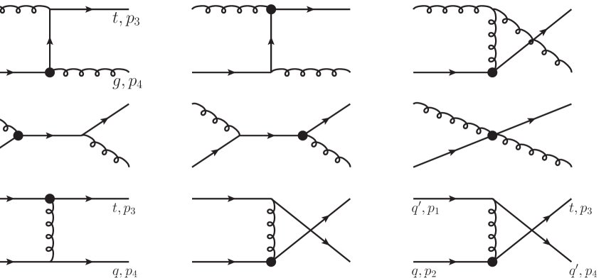
The LO squared amplitudes for the corresponding subprocesses in four dimensions are
| (3) |
respectively, where is the top quark mass, and , the colors and spins of the outgoing particles have been summed over, and the colors and spins of the incoming ones have been averaged over, , , and are Mandelstam variables, which are defined as
| (4) |
After the phase space integration, the LO partonic cross sections are given by
| (5) |
The LO total cross section at hadron colliders is obtained by convoluting the partonic cross section with the parton distribution functions (PDFs) for the proton (antiproton):
| (6) |
where is the factorization scale.
III Next-to-leading order QCD corrections
The NLO corrections to the single top production via the FCNC couplings consist of the virtual corrections, generated by loop diagrams of colored particles, and the real corrections with the radiation of a real gluon or a massless (anti)quark. We carried out all the calculations in the ’t Hooft-Feynman gauge and used the dimensional regularization (DREG) scheme 'tHooft:1972fi in dimensions to regularize all the divergences. Moreover, for the real corrections, we used the dipole subtraction method with massive partons Catani:2002hc to separate the infrared (IR) divergences, which is convenient for the case of massive Feynman diagrams and provides better numerical accuracy.
III.1 Virtual corrections
The virtual corrections for the single top production via the FCNC couplings include the box diagrams, triangle diagrams and self-energy diagrams as shown in Figs. 2-3 and Fig. 4 for the and initial state subprocess, respectively. For simplicity we did not show the diagrams that only differ by the exchange of identical external particles. The loop diagrams for the and initial state subprocess can be obtained from Figs. 2-3 and Fig. 4 by crossing symmetry, and the ones for are just part of Fig. 4.
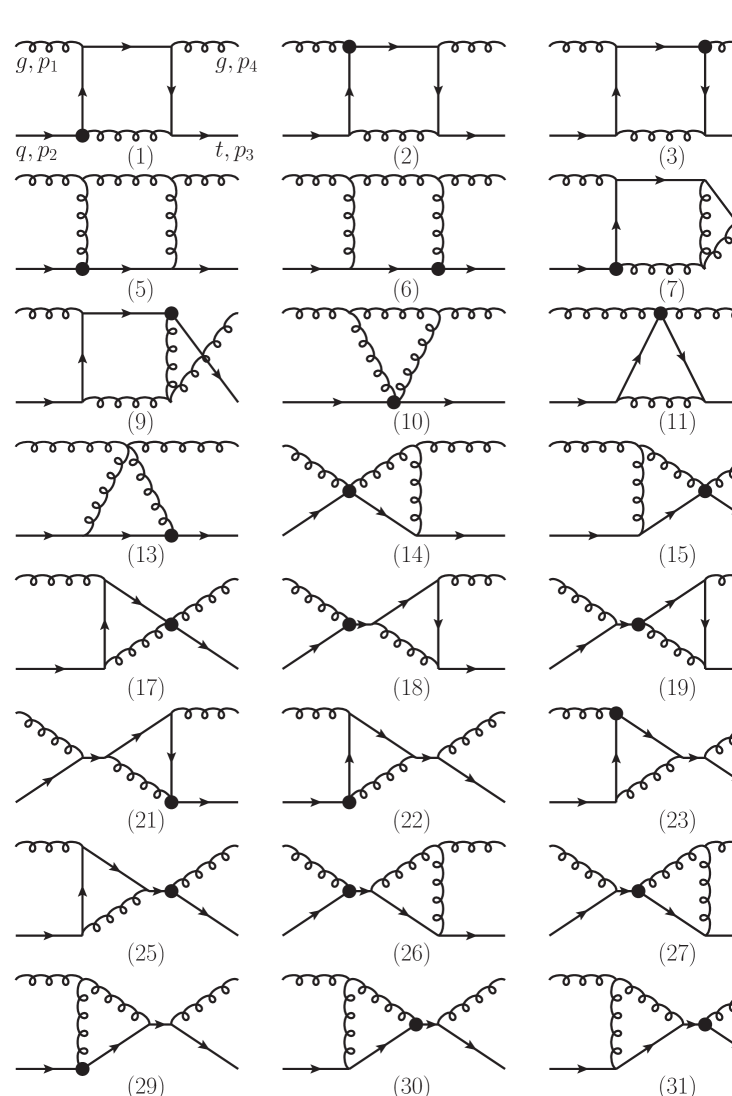
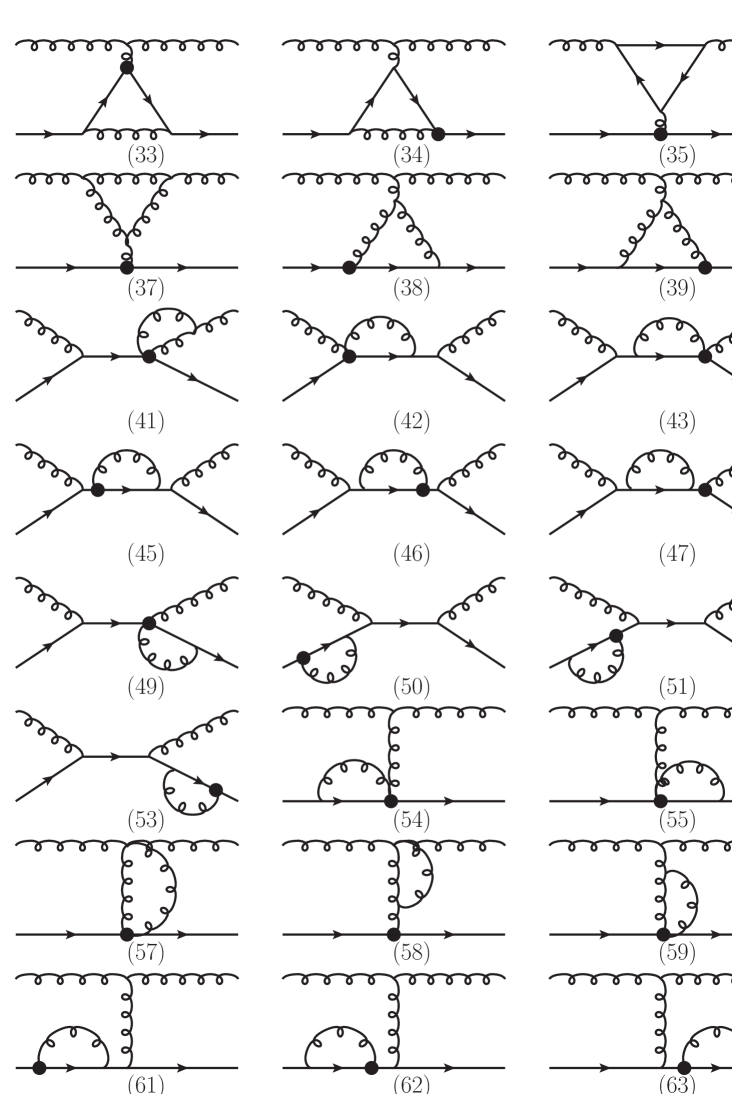
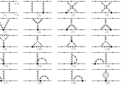
All the ultraviolet (UV) divergences appearing in the loop diagrams are renormalized by introducing counterterms for the wave functions and mass of the external fields (), and the coupling constants (). We define these counterterms according to the following conventions. For the external fields, we fix all the renormalization constants using on-shell subtraction, and, therefore, they also have IR singularities:
| (7) |
where and . For the renormalization of , we use the scheme modified to decouple the top quark Collins:1978wz , i.e. the first light flavors are subtracted using the scheme, while the divergences associated with the top quark loop are subtracted at zero momentum:
| (8) |
Thus, the renormalized strong coupling constant evolves with light flavors in this scheme. Finally, for the renormalization constants of the FCNC couplings , we adopt the scheme and adjust it to cancel the remaining UV divergences exactly:
| (9) |
and the running of the FCNC couplings are given by Zhang:2009jj
| (10) |
with .
The squared amplitudes of the virtual corrections are
| (11) |
where denote the amplitudes for the i-th loop diagram in Figs. 2-3 or Fig. 4, and are the corresponding counterterms. All the one-loop integrals in the loop amplitudes can be calculated using the standard Passarino-Veltman techniques Denner:1991kt , and the explicit expressions for the scalar integrals containing IR divergences can be found in Ref. Ellis:2007qk . In Eq. (11), all the UV divergences cancel each other, leaving the remaining IR divergences and the finite terms. Because of the limited space, we do not shown the lengthy explicit expressions of the virtual corrections here. The IR divergence of the virtual corrections can be written as
| (12) |
where , and are the squared Born amplitudes given in Eq. (II). The terms can not be factorized in a trivial way due to the nontrivial color structures of the LO amplitudes, and can be expressed as combinations of the LO color correlated squared amplitudes as shown in the next section.
III.2 Real corrections
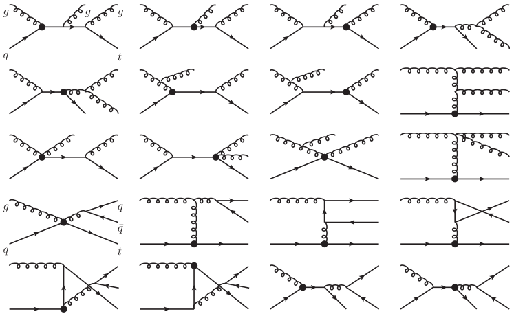
At the NLO the real corrections consist of the radiations of an additional gluon or massless (anti)quark in the final states, including the subprocesses
| (13) |
as shown in Fig. 5. It should be noted that in our NLO calculations we did not include the contributions from the SM on-shell production of the top pair with subsequent rare decay of one top quark, , which provide the same signature as the single top production via the FCNC couplings and can be calculated separately. We will discuss these contributions in the numerical results.
Before performing the numerical calculations, we need to extract the IR divergences in the real corrections. In the dipole formalism this is done by subtracting some dipole terms from the real corrections to cancel the singularities and large logarithms exactly, and then the real corrections become integrable in four dimensions. On the other hand, these dipole subtraction terms are analytically integrable in dimensions over one-parton subspaces, which give poles that represent the soft and collinear divergences. Then we can add them to the virtual corrections to cancel the poles, and ensure the virtual corrections are also integrable in four dimensions. This whole procedure can be illustrated by the formula Catani:2002hc :
| (14) |
where is the number of final state particles at the LO, and is a sum of the dipole terms. Besides, at hadron colliders, we have to include the well-known collinear subtraction counterterms in order to cancel the collinear divergences arising from the splitting processes of the initial state massless partons. Here we use the scheme and the corresponding NLO PDFs.
For the process with two initial state hadrons, the dipole terms can be classified into four groups, the final-state emitter and final-state spectator type,
| (15) |
the final-state emitter and initial-state spectator type,
| (16) |
the initial-state emitter and final-state spectator type,
| (17) |
and the initial-state emitter and initial-state spectator type,
| (18) |
where and are the initial and final state partons, and T and V are the color charge operators and dipole functions acting on the LO amplitudes, respectively. The explicit expressions for , and V can be found in Ref. Catani:2002hc . The integrated dipole functions together with the collinear counterterms can be written in the following factorized form
| (19) | |||||
where is the momentum fraction of the splitting parton, contains all the factors apart from the squared amplitudes, I, P, and K are insertion operators defined in Catani:2002hc . For simplicity, in all the above formulas we do not show the jet functions that define the observables and are included in our numerical calculations.
The operators P and K provide finite contributions to the NLO corrections, and only the operator I contains the IR divergences
| (20) | |||||
with
| (21) |
where , , and . And , , , and are kinematic variables defined as follows
| (22) |
When inserting Eq. (20) into the LO amplitudes for the and subprocesses as shown in Eq. (19), we can see that the IR divergences, including the terms, can be written as combinations of the LO color correlated squared amplitudes and all the IR divergences from the virtual corrections in Eq. (III.1) are canceled exactly, as we expected.
IV Numerical Results
In the numerical calculations, we investigate the NLO QCD effects on the total cross sections, the scale dependence, and several important distributions at both the Tevatron and LHC. For the single top production via the FCNC couplings at the NLO, the final state consists of a top quark plus one or two partons which may form jets. We use the cone jet algorithm with , and require the jet to have and . We require that there is at least one jet in the final state, which means the signal we considered is , unlike the direct top production. All the input parameters are taken to be Amsler:2008zzb :
| (23) |
The running QCD coupling constant is evaluated at the three-loop order Amsler:2008zzb and the CTEQ6M PDF set Pumplin:2002vw is used throughout the calculations of the NLO (LO) cross sections. Both the renormalization and factorization scales are fixed to the top quark mass unless specified. We have performed two independent calculations for the virtual corrections and the integrated dipole terms, and used the modified MadDipole Frederix:2008hu package to generate the Fortran code for the real corrections. The numerical results of the two groups are in good agreement within the expected accuracy of our numerical program.
| FCNC coupling | (LO) | (NLO) | (LO) | (NLO) |
|---|---|---|---|---|
| LHC pb | 6.77 | 8.41 | 1.10 | 1.49 |
| Tevatron fb | 86 | 129 | 6.2 | 10.2 |
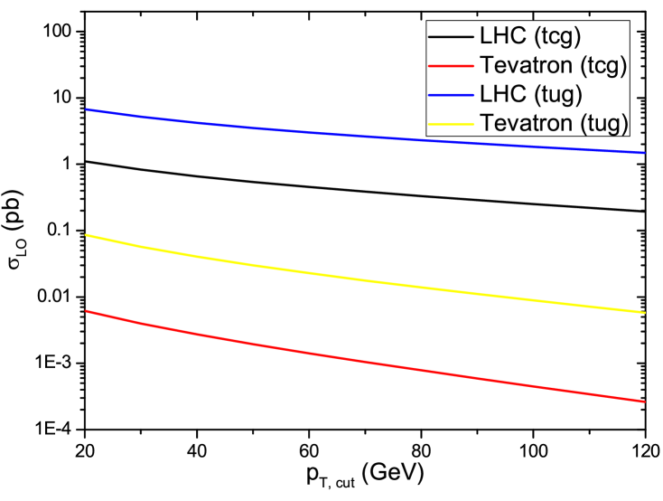
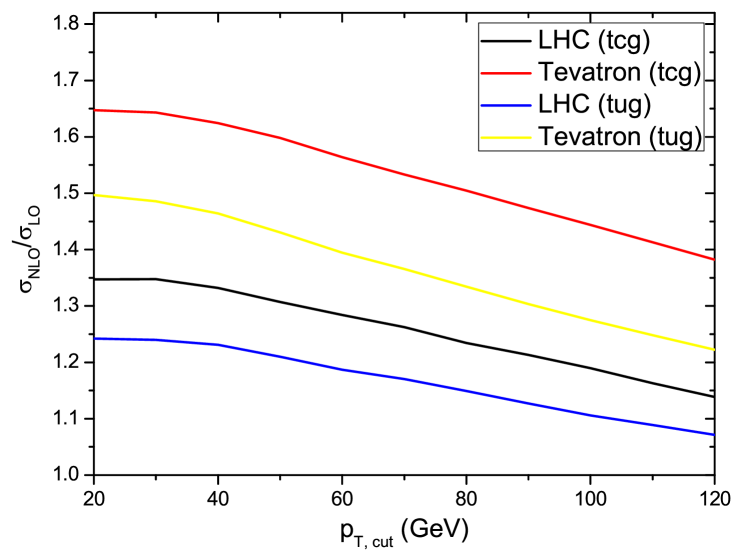
In Table 1, we list some typical numerical results of the LO and NLO total cross sections for the single top quark production via the FCNC couplings. We can see that the cross sections can reach about 8 pb and 1 pb at the LHC, for the and coupling, respectively. But if we take the FCNC coupling values to the experimental upper limits Aaltonen:2008qr , then the cross sections can reach as large as several tens of pb. In Fig. 6 we present the LO total cross sections and the K factors as functions of the leading jet transverse momentum cut, respectively. It can be seen that, for the coupling the NLO corrections can enhance the total cross sections by about 60% and 30%, and for the coupling by about 50% and 20% at the Tevatron and LHC, respectively. And the K factors decrease with the increasing transverse momentum cut. In Sec. III.2 we mentioned that the SM on shell production of the top pair with subsequent decay also contributes to the same final state as the FCNC single top production. According to Ref. Zhang:2008yn , the former contributions are about pb and pb at the Tevatron and LHC, respectively, for our chosen FCNC coupling values. Compared with the results in Table 1, we can see that these contributions are negligibly small for the coupling, but can reach about 10% of the LO total cross sections for the coupling at both the Tevatron and LHC.
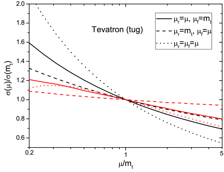
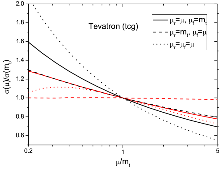
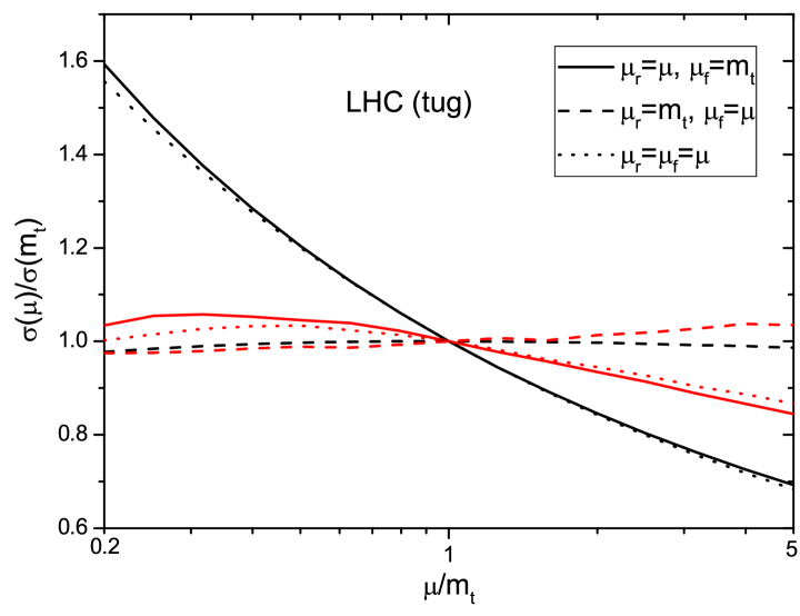
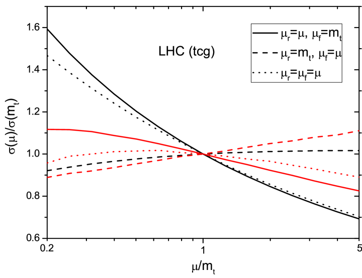
In Figs. 7 and 8 we show the scale dependence of the LO and NLO total cross section for three cases: (1) the renormalization scale dependence , (2) the factorization scale dependence , and (3) total scale dependence . It can be seen that the NLO corrections reduce the scale dependence significantly for all three cases, which make the theoretical predictions more reliable. For example, at the Tevatron for the coupling, when the scale varies from to , the variations of the total cross sections are 90% and 40% for case (1), 50% and 20% for case (2), and 150% and 50% for case (3) at the LO and NLO, respectively. Note that, from Fig. 8 it seems that the NLO corrections did not reduce the factorization scale dependence at the LHC. This is because the PDFs of the two incoming partons have opposite trends with the increasing factorization scale and the scale dependence cancel each other at the LO, but there is no such cancellation at the NLO. In order to further explain this scenario, in Fig. 9 we plot the factorization scale dependence of the initial state subprocess at the LHC, which contributes about 90% of the LO total cross section for the coupling. It can be seen that, if we fix the factorization scale of one incoming parton and only change another one, the NLO corrections indeed improve the factorization scale dependence.
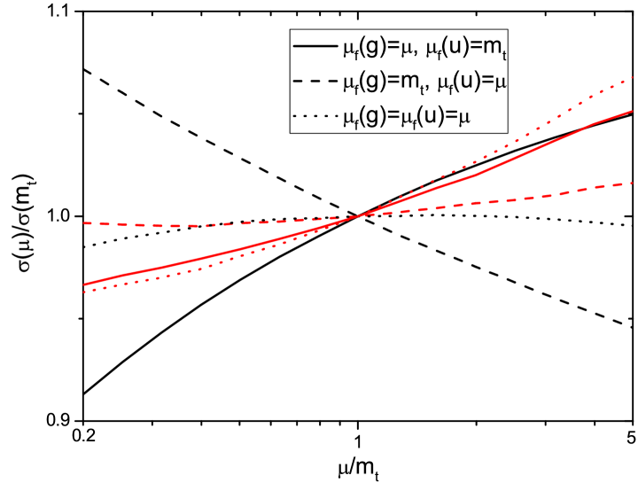
Figure 10 shows the transverse momentum distributions of the leading jet for the single top production via the FCNC couplings together with the SM t-channel single top production, which is the main SM background of our process. We can see that the distributions of the single top production via the FCNC couplings decrease more quickly than the SM ones with the increasing , and the NLO corrections increase the distributions of the FCNC single top production, especially in the low regions. In Fig. 11 we show the pseudorapidity distributions of the leading jet. For the FCNC single top production, the distributions decrease with the increasing pseudorapidity at both the Tevatron and LHC, while for the SM ones the distributions are almost flat at the Tevatron and increase at the LHC. The NLO corrections increase the distributions by almost the same amount in all the regions.
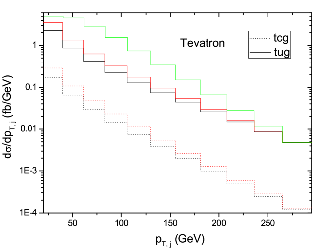
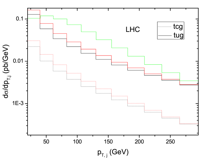
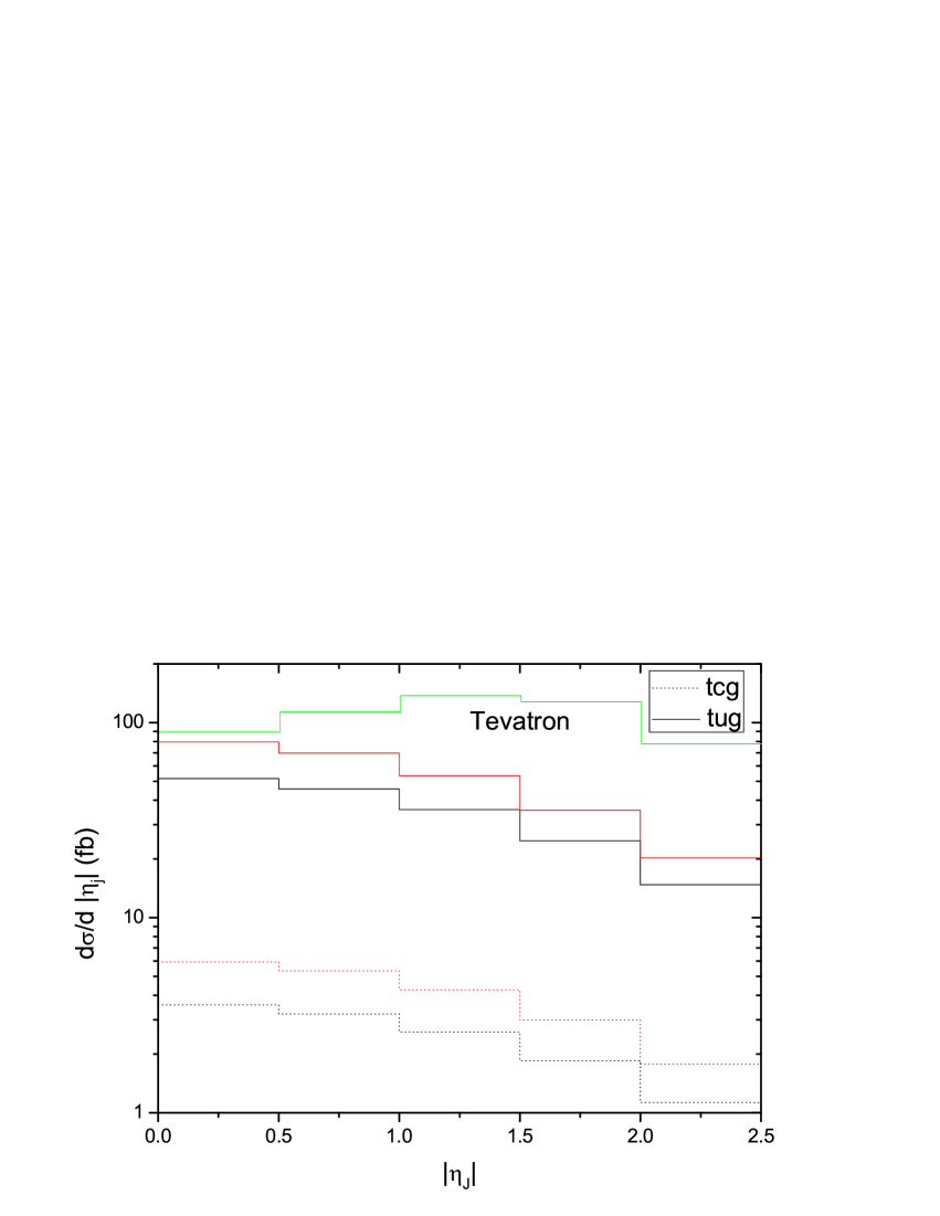
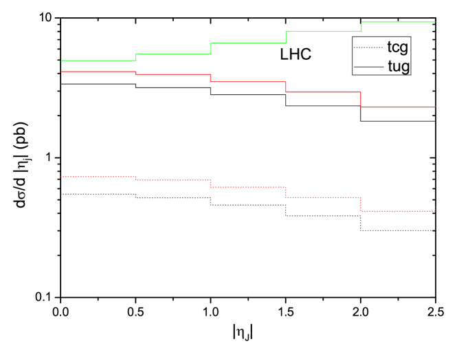
Fig. 12 gives the top quark energy distributions. We can see that the SM ones decrease faster than the one of FCNC coupling with the increasing top quark energy. Figure 13 shows the invariant mass distributions of the top quark and the leading jet. The shapes for the FCNC single top production are different from the SM ones, where there is a peak in the middle region. The NLO corrections do not change the shapes of these two distributions.
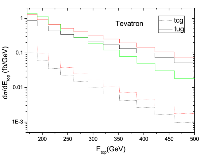
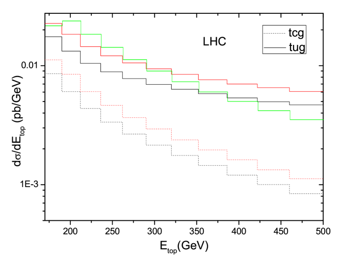
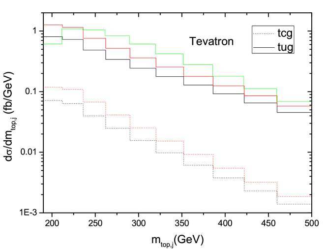
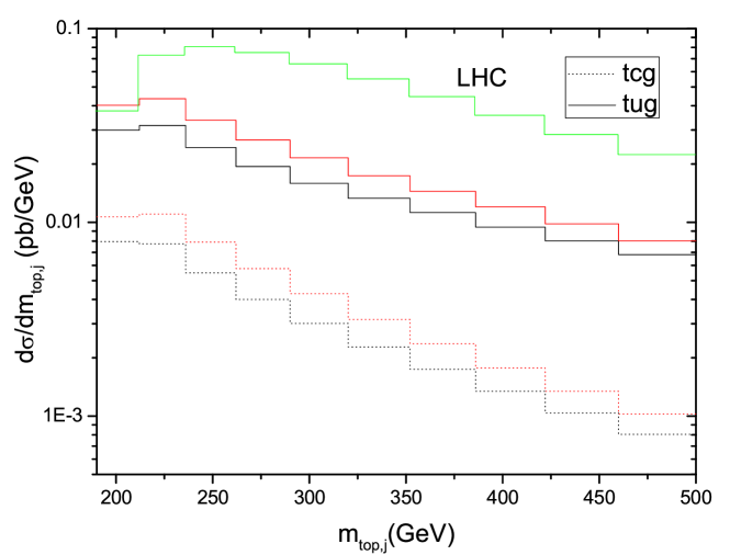
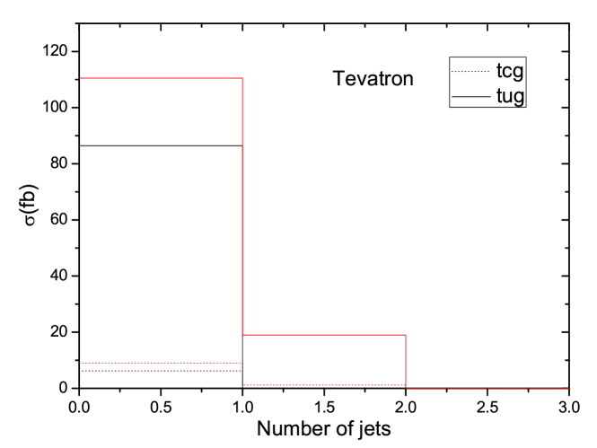
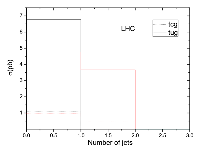
Figure 14 shows the jet multiplicities distributions of the FCNC single top production. At the LO there is only one jet in the final state, while at the NLO there may be two jets. For example, at the LHC, for the coupling the LO one jet cross section is 6.7 pb, and the NLO corrections reduce the one jet cross section to 4.8 pb and increase the two jets cross section to 3.7 pb, which is about 50% of the LO total cross section.
V Conclusions
In conclusion, we have investigated the NLO QCD effects on the single top productions induced by model-independent FCNC couplings at both the Tevatron and LHC. Our results show that, for the coupling the NLO corrections can enhance the total cross sections by about 60% and 30%, and for the coupling by about 50% and 20% at the Tevatron and LHC, respectively, which means that the NLO corrections can increase the experimental sensitivity to the FCNC couplings by about 10%30%. Moreover, the NLO corrections reduce the dependence of the total cross sections on the renormalization or factorization scale significantly, which lead to increased confidence on the theoretical predictions. Besides, we also evaluate the NLO corrections to several important kinematic distributions, i.e., the transverse momentum and pseudorapidity of the leading jet, energy of the top quark, jet multiplicities, and invariant mass of the leading jet and top quark. We find that for most of them the NLO corrections are almost the same and do not change the shape of the distributions.
Acknowledgements.
We would like to thank Tao Han for useful discussions. This work was supported in part by the National Natural Science Foundation of China, under Grants No. 10721063, No. 10975004 and No. 10635030.References
- (1) S. L. Glashow, J. Iliopoulos and L. Maiani, Phys. Rev. D 2 (1970) 1285.
- (2) J. A. Aguilar-Saavedra, Acta Phys. Polon. B 35 (2004) 2695.
- (3) F. del Aguila, J. A. Aguilar-Saavedra and R. Miquel, Phys. Rev. Lett. 82 (1999) 1628; J. A. Aguilar-Saavedra, Phys. Rev. D 67 (2003) 035003 [Erratum-ibid. D 69 (2004) 099901].
- (4) T. P. Cheng and M. Sher, Phys. Rev. D 35 (1987) 3484; M. E. Luke and M. J. Savage, Phys. Lett. B 307 (1993) 387; D. Atwood, L. Reina and A. Soni, Phys. Rev. D 55 (1997) 3156; S. Bejar, J. Guasch and J. Sola, Nucl. Phys. B 600 (2001) 21.
- (5) C. S. Li, R. J. Oakes and J. M. Yang, Phys. Rev. D 49 (1994) 293 [Erratum-ibid. D 56 (1997) 3156]; J. L. Lopez, D. V. Nanopoulos and R. Rangarajan, Phys. Rev. D 56 (1997) 3100; G. M. de Divitiis, R. Petronzio and L. Silvestrini, Nucl. Phys. B 504 (1997) 45; J. M. Yang, B. L. Young and X. Zhang, Phys. Rev. D 58 (1998) 055001; J. Guasch and J. Sola, Nucl. Phys. B 562 (1999) 3; G. Eilam, A. Gemintern, T. Han, J. M. Yang and X. Zhang, Phys. Lett. B 510 (2001) 227; J. j. Cao, Z. h. Xiong and J. M. Yang, Phys. Rev. Lett. 88 (2002) 111802; J. J. Liu, C. S. Li, L. L. Yang and L. G. Jin, Phys. Lett. B 599 (2004) 92.
- (6) H. Davoudiasl and T. G. Rizzo, Phys. Lett. B 512 (2001) 100; P. M. Aquino, G. Burdman and O. J. P. Eboli, Phys. Rev. Lett. 98 (2007) 131601; S. Casagrande, F. Goertz, U. Haisch, M. Neubert and T. Pfoh, JHEP 0810 (2008) 094; J. Gao, C. S. Li, X. Gao and Z. Li, Phys. Rev. D 78 (2008) 096005.
- (7) H. Hong-Sheng, Phys. Rev. D 75 (2007) 094010; X. Wang, Y. Zhang, H. Jin and Y. Xi, Nucl. Phys. B 810 (2009) 226; X. F. Han, L. Wang and J. M. Yang, arXiv:0903.5491 [hep-ph].
- (8) X. L. Wang, G. R. Lu, J. M. Yang, Z. J. Xiao, C. X. Yue and Y. M. Zhang, Phys. Rev. D 50 (1994) 5781; G. Burdman, Phys. Rev. Lett. 83 (1999) 2888; C. x. Yue, G. r. Lu, Q. j. Xu, G. l. Liu and G. p. Gao, Phys. Lett. B 508 (2001) 290; J. j. Cao, G. l. Liu and J. M. Yang, Phys. Rev. D 70 (2004) 114035; J. j. Cao, G. l. Liu, J. M. Yang and H. j. Zhang, Phys. Rev. D 76 (2007) 014004.
- (9) W. Buchmuller and D. Wyler, Nucl. Phys. B 268 (1986) 621.
- (10) J. A. Aguilar-Saavedra, Nucl. Phys. B 812 (2009) 181.
- (11) M. Hosch, K. Whisnant and B. L. Young, Phys. Rev. D 56 (1997) 5725.
- (12) E. Malkawi and T. M. P. Tait, Phys. Rev. D 54 (1996) 5758; P. M. Ferreira and R. Santos, Phys. Rev. D 73 (2006) 054025.
- (13) T. Han, M. Hosch, K. Whisnant, B. L. Young and X. Zhang, Phys. Rev. D 58 (1998) 073008.
- (14) J. Carvalho et al. [ATLAS Collaboration], Eur. Phys. J. C 52 (2007) 999.
- (15) T. Aaltonen et al. [CDF Collaboration], Phys. Rev. Lett. 102 (2009) 151801.
- (16) V. M. Abazov et al. [D0 Collaboration], Phys. Rev. Lett. 99 (2007) 191802.
- (17) J. J. Liu, C. S. Li, L. L. Yang and L. G. Jin, Phys. Rev. D 72 (2005) 074018; L. L. Yang, C. S. Li, Y. Gao and J. J. Liu, Phys. Rev. D 73 (2006) 074017.
- (18) J. J. Zhang, C. S. Li, J. Gao, H. Zhang, Z. Li, C. P. Yuan and T. C. Yuan, Phys. Rev. Lett. 102 (2009) 072001.
- (19) G. ’t Hooft and M. J. G. Veltman, Nucl. Phys. B 44 (1972) 189.
- (20) S. Catani, S. Dittmaier, M. H. Seymour and Z. Trocsanyi, Nucl. Phys. B 627 (2002) 189.
- (21) J. C. Collins, F. Wilczek and A. Zee, Phys. Rev. D 18 (1978) 242.
- (22) J. J. Zhang, C. S. Li, J. Gao and H. X. Zhu, in preparation.
- (23) A. Denner, Fortsch. Phys. 41 (1993) 307.
- (24) R. K. Ellis and G. Zanderighi, JHEP 0802 (2008) 002.
- (25) C. Amsler et al. [Particle Data Group], Phys. Lett. B 667 (2008) 1.
- (26) J. Pumplin, D. R. Stump, J. Huston, H. L. Lai, P. M. Nadolsky and W. K. Tung, JHEP 0207 (2002) 012.
- (27) R. Frederix, T. Gehrmann and N. Greiner, JHEP 0809 (2008) 122.