Johannes Gutenberg University Mainz, 55099 Mainz, Germany
11email: {hsu, wolfgang.paul, theodora, kurt.binder}@uni-mainz.de 22institutetext: Institute for Physics,
Martin-Luther University Halle-Wittenberg, 06120 Halle, Germany
22email: wolfgang.paul@physik.uni-halle.de
Phase Transitions and Relaxation Processes in Macromolecular Systems: The Case of Bottle-brush Polymers
Abstract
As an example for the interplay of structure, dynamics, and phase behavior of macromolecular systems, this article focuses on the problem of bottle-brush polymers with either rigid or flexible backbones. On a polymer with chain length , side-chains with chain length are endgrafted with grafting density . Due to the multitude of characteristic length scales and the size of these polymers (typically these cylindrical macromolecules contain of the order of 10000 effective monomeric units) understanding of the structure is a challenge for experiment. But due to excessively large relaxation times (particularly under poor solvent conditions) such macromolecules also are a challenge for simulation studies. Simulation strategies to deal with this challenge, both using Monte Carlo and Molecular Dynamics Methods, will be briefly discussed, and typical results will be used to illustrate the insight that can be gained.
(a)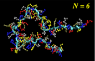 (b)
(b)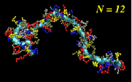
(c)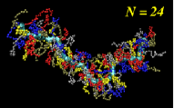 (d)
(d)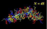
1 Introduction
The so-called “bottle-brush polymers” consist of a long macromolecule serving as a “backbone” on which many flexible side chains are densely grafted [1, 2]. Since the chemical synthesis of such complex polymeric structures has become possible, these molecular bottle-brushes have found much interest for various possible applications: the structure reacts very sensitively to changes of solvent quality (due to change of temperature of the solution, pH value, etc.), enabling the use of these molecules as sensors or actuators on the nanoscale [3, 4]. For some conditions these bottle-brush molecules behave like stiff cylindrical rods, and hence they can serve as building blocks of supramolecular aggregates, or show orientational order in solution as nematic liquid crystals do. On the other hand, these molecular bottle-brushes are also very “soft”, i.e, they show only very small resistance to shear deformation; bottle-brush molecules of biological origin such as aggrecan which occurs in the cartilage of mammalian (including human!) joints are indeed held responsible for the excellent lubrication properties (reducing frictional forces) in such joints [5].
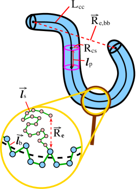
However, for being able to control the function of these complex macromolecules one must be able to control their structure, i.e., one must understand how the structure depends on various parameters of the problem: chain length of the “backbone”, chain length of the side chains, grafting density of the side chains along the backbone, solvent quality, just to name the most important ones of these parameters. This is the reason why computer simulations are needed in order to understand such bottle-brushes: even in the case of good solvent, the structure of these objects is very complicated as the snapshot pictures [6, 7] (Fig. 1) of the simulated models show, and there occur a multitude of characteristic length scales (Fig. 2) [6, 7] that are needed to describe the structure; it is very difficult to extract this information from experiment, and hence simulations are valuable here as they can yield a far more detailed picture.
Of course, the large size of these bottle-brush polymers (even the coarse-grained models described in the following sections contain of the order of several thousand or even more than 10000 effective monomers per polymer) is a serious obstacle for simulation, too; in fact, developing efficient models and methods for the simulation of macromolecular systems is a longstanding and important problem [8, 9]. We hence shall address this issue of proper choice of both suitable models and efficient algorithms in the next sections.
(a)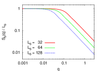 (b)
(b)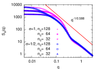
(c)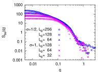 (d)
(d)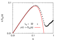
2 Bottle-brush polymers with rigid backbones in good solvents
If one assumes the backbone of the bottle-brush to be completely stiff, the problem is reduced to grafting side chains of length to a straight line. Although this limiting case seems somewhat artificial, from the point of view that one wishes to model real systems, it is a very useful test case: there is no reason to assume that approximations that already fail in this rather simple limit become accurate for the more complicated case of flexible backbones; moreover, this case is rather simple to simulate, and the analysis of the simulation data is relatively straightforward.
For the study of this case, polymers were simply represented as standard self-avoiding walks on the simple-cubic lattice (i.e., beads of the chains are occupied lattice sites, connected by nearest-neighbor links on the lattice, and multiple occupancy of sites is forbidden [8, 9]).
As a simulation method, pruned-enriched Rosenbluth methods (PERM) [10, 11] were used [12]. In the Rosenbluth method, all side chains are grown simultaneously step by step, choosing only from sites which are not yet occupied, and the statistical weight of the polymer configuration is computed recursively. In the PERM algorithm, one does not grow a single polymer at a time, but a large “population” of equivalent chains is grown simultaneously but from time to time configurations with very low statistical weight are killed, and configurations with large statistical weight are “cloned” (“go with the winners”strategy [10]). The advantage is that (unlike dynamic Monte Carlo algorithms [8, 9]) this method does not suffer from “critical slowing down” when gets large, and data for all (up to the maximum value studied) are obtained in a single simulation (see [11] for more details).
Now one hypothesis popular in most experimental studies (e.g. [13, 14]) is the factorization approximation [15] for the structure factor (that describes the small angle scattering intensity of neutrons, X-rays or light from dilute solutions of bottle-brushes polymers) into a contribution due to the backbone () and due to the side chains
| (1) |
where is the absolute value of the scattering wave vector. In the last step the side chain scattering was approximated by . This cross sectional scattering is in turn approximated related to the radial density perpendicular to the cylinder axis at which the side chains are grafted as (the constant ensures proper normalization [12])
| (2) |
Obviously, Eq. (1) neglects interference effects due to correlations between the monomer positions in the side chains and in the backbone. Writing the scattering due to the monomers in the side chains as the average of a square {Eq. (2)} ignores correlations in the occupation probability in the -direction along the bottle-brush axis. All such correlations do contribute to the actual structure factor, of course, when it is computed from its definition,
| (3) |
Here is an occupation variable, if the site is occupied by a bead, and zero otherwise, and the sums extend over all monomers (in the side chains and in the backbone).
In the simulation, one can go beyond experiment by not only recording the total scattering , but also the contributions , and individually (Fig. 3). One can see that the approximation leads to a relative error of the order of a few % only (cf. the difference in ordinate scales between parts b) and c), while the assumption [with Eq. (2)] leads to appreciable errors at large (see part d)). Therefore the use of Eqs. (1), (2) to analyze experiments can lead to appreciable errors, when one wishes to predict [12] the radial density distribution .
3 Bottle-brushes with flexible backbones in good solvents
In the case of flexible backbones, the PERM algorithm no longer provides an efficient sampling of configuration space; there “dynamic” Monte Carlo algorithms are used, but with “unphysical moves” allowing chain intersections and large configurational changes in a single step, as achieved by the Pivot algorithm [8, 9]. Using the bond fluctuation model [8, 9], the “L26 algorithm” [16] was used [17] for local moves allowing bond intersection and nevertheless respecting excluded volume. In this way well-equilibrated data for systems with up to monomers at the backbone and up to monomers in the side chains could be studied (for ). Examples of snapshot pictures have already been given in Fig. 1.
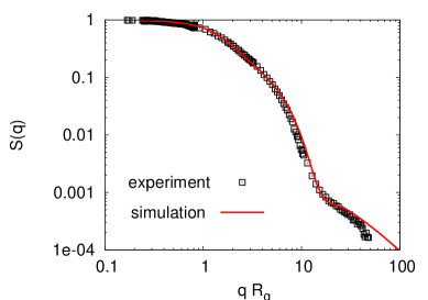
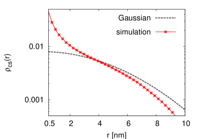
Adjusting the physical meaning of the lattice spacing to correspond to 0.263 nm, the structure factor of the simulated model matches almost perfectly an experimental result [13] (for slightly different numbers of chemical monomers, , ; this difference is irrelevant, since there is no one-to-one correspondence between covalent bonds and the “effective bonds” of the model) see [7] Fig. 4. From the simulation one can directly extract the cross-sectional density profile and compare it [7] to the approximate experimental result (Fig. 5), which was obtained from fitting to Eqs. (1), (2) [13]. One sees that the analysis of the experiment could predict roughly correctly the distance on which the profile decays to zero, but does not account for its precise functional form. A further interesting finding [7, 17] is the result that the persistence length (cf. Fig2) depends strongly [7] on (at least if one uses the textbook definitions [18]), and hence is not a useful measure of local chain stiffness.
4 Bottle-brushes in poor solvents
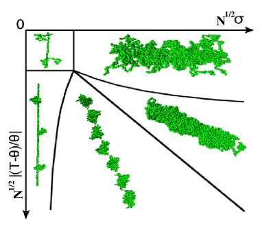
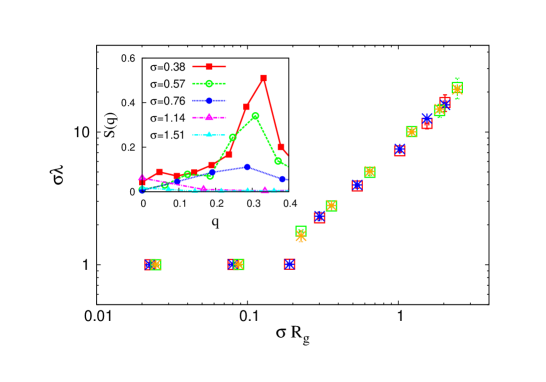
While isolated single chains in dilute solution collapse to dense globules [18] when the temperature is lowered below the Theta temperature , for a bottle-brush the constraint of the chains being grafted to a backbone leads to an interesting diagram of states, considering and as variables (Fig. 6) [19]. Near and the side chains collapse to dense globules when . For and one has a cylindrical structure (as in the previous sections) which collapses to a dense cylinder when . However, interestingly at intermediate grafting densities and a laterally inhomogeneous “pearl necklace-structure” was predicted [19].
This problem can neither be studied efficiently by the PERM method nor by the bond fluctuation algorithm of Sec. 3 - both methods get very inefficient for dense polymer configurations. Thus, instead Molecular Dynamics simulations of the standard Grest-Kremer-type bead-spring model [8, 9] were carried out [20]. Fig. 7 shows [20] characteristic wavelength plotted vs. grafting density . One finds that for small a trivial periodicity given by occurs, while for () the periodicity is essentially independent of , given by about that . Of course, mapping out the phase behavior precisely for a wide range of , and is a formidable problem, due to very long relaxation times of the collapsed states in Fig. 6.
5 Concluding Remarks
The above examples have illustrated that polymers with complex architecture pose challenging problems with respect to their structure and thermodynamics. Investigation of their relaxation behavior is another interesting problem, to be tackled in the future. The above examples have also illustrated the need to carefully adjust both the model and the algorithm to the problems one wants to deal with.
Acknowledgments
One of us (H.-P. Hsu) received support from the DFG (SFB625/A3), another (P. E. Theodorakis) from the MPG via a Max-Planck Fellowship of the MPI-P. We are grateful to the NIC Jülich for computer time at the JUMP and SoftComp cluster.
References
- [1] M. Zhang and A. H. E. Müller, \JournalJ. Polym. Sci., Part A, Polym. Chem.4334612005.
- [2] S. S. Sheiko, B. S. Sumerlin, and K. Matyjaszewski, \JournalProg. Polym. Sci.337592008.
- [3] T. Stephan, S. Muth, and M. Schmidt, \JournalMacromolecules3598572002.
- [4] C. Li, N. Gunari, K. Fischer, A. Janshoff, and M. Schmidt, \JournalAngew. Chem. Int. Ed.4311012004.
- [5] J. Klein, \JournalScience323472009.
- [6] H.-P. Hsu, W. Paul, and K. Binder, INSIDE (2009, in press).
- [7] H.-P. Hsu, W, Paul, S. Rathgeber and K. Binder, preprint.
- [8] K. Binder (ed.) Monte Carlo and Molecular Dynamics Simulations in Polymer Science (Oxford Univ. Press, New York, 1995).
- [9] N. Attig, K. Binder, H. Grubmüller, and K. Kremer (eds.) Computational Soft Matter: From Synthetic Polymers to Proteins (NIC, Jülich, 2004).
- [10] P. Grassberger, \JournalPhys. Rev. E56 3682 1997.
- [11] H.-P. Hsu, W. Paul, and K. Binder, \JournalMacromol. Theory Simul. 16 660 2007.
- [12] H.-P. Hsu, W. Paul, and K. Binder, \JournalJ. Chem. Phys. 129 204904 2008.
- [13] S. Rathgeber, T. Pakula, A. Wilk, K. Matyjaszewski, and K. L. Beers, \JournalJ. Chem. Phys. 122 124904 2005.
- [14] B. Zhang, F. Gröhn, J. S. Pedersen, K. Fischer, and M. Schmidt, \JournalMacromolecules 39 8440 2006.
- [15] J. S. Pedersen and P. Schustenberger, \JournalMacromolecules 29 7602 1996.
- [16] J. P. Wittmer, P. Beckrich, H. Meyer, A. Cavallo, A. Johner, and J. Baschnagel, \JournalPhys. Rev. E76 011803 2007.
- [17] H.-P. Hsu, K. Binder, and W. Paul, Phys. Rev. Lett. (2009, in press).
- [18] A. Yu Grosberg and A. R. Khokhlov, Statistical Physics of Macromolecules (AIP Press, New York, 1994).
- [19] S. S. Sheiko, O. V. Borisov, S. A, Prokhorova, and M. Möller, \JournalEur. Phys. J. E. 13 125 2004.
- [20] P .E. Theodorakis, W. Paul, and K. Binder, preprint.