How to define physical properties of unstable particles

Abstract

In the framework of effective quantum field theory we address the definition of physical quantities characterizing unstable particles. With the aid of a one-loop calculation, we study this issue in terms of the charge and the magnetic moment of a spin-1/2 resonance. By appealing to the invariance of physical observables under field redefinitions we demonstrate that physical properties of unstable particles should be extracted from the residues at complex (double) poles of the corresponding $S$-matrix.

I Introduction

The question how to define a theory of unstable particles which is consistent with general requirements of a relativistic quantum field theory has a long history (see, e.g., Refs. Matthews:1958sc ; Matthews:1959sy ; Jacob:1961zz for early work). In the beginning, the discussion primarily focussed on the definition of the mean mass and the mean lifetime as static characteristics of an unstable particle. In the early 1990s, this issue attracted considerable renewed attention in the context of the Standard Model. For instance, in Refs. Willenbrock:1990et ; Valencia:1990jp an example was given in the scalar sector showing the field-redefinition dependence of the mass once defined as the zero of the real part of the inverse propagator. Such a definition corresponds to a relativistic Breit-Wigner mass parameter. Furthermore, for the $Z$ boson it was shown in Refs. Sirlin:1991fd ; Sirlin:1991rt ; Willenbrock:1991hu ; Gegelia:1992kj ; Gambino:1999ai that, at two-loop order, the Breit-Wigner mass is gauge-parameter dependent. In contrast, the mass of an unstable particle defined through the real part of the pole of the propagator is field-redefinition and gauge-parameter independent 'tHooft:1972ue ; Lee:1972fj ; Balian:1976vq and therefore qualifies as a physical quantity.

As there is no fundamental dynamical theory of hadron resonances the problem of field-redefinition invariance and gauge-parameter (in)dependence received little attention for these unstable particles Willenbrock:1991hu . The characteristic properties of hadron resonances eventually have to be described by QCD. With the progress of lattice techniques Wittig:2008zz ; Alexandrou:2008bn ; Braun:2009jy ; Boinepalli:2009sq and, especially, the low-energy effective theories (EFT) of QCD (see, e.g., Weinberg:1979kz ; Gasser:1983yg ; Gasser:1988rb ; Scherer:2002tk ; Pascalutsa:2006up ; Scherer:2009bt and references therein) it is timely to reinvestigate the definition of physical characteristics of resonances. In the present work we study this issue in terms of the charge and the magnetic moment of a spin-1/2 resonance. The choice of electromagnetic properties is motivated by the fact that there already exists an extensive experimental and theoretical program for investigating resonance photon decay amplitudes and nucleon resonance transition form factors (see, e.g., Tiator:2003uu ; Burkert:2004sk ; Capstick:2007tv ; Burkert:2008mw ). Moreover, experiments aiming at the extraction of magnetic moments of excited baryons have already been performed or are planned (see, e.g., Ref. Kotulla:2008zz for an overview).

II The model and definitions

In order to keep the technicalities as simple as possible, while at the same time studying a sufficiently non-trivial physics case, we consider a toy model for a positively charged, unstable heavy fermion ($\Psi$) (“resonance”) which may decay into a positively charged, stable light fermion $(\psi)$ (“proton”) and a stable, neutral pseudoscalar $\phi$ (“neutral pion”). We make use of the following effective Lagrangian,

$$\mathcal{L}_{\rm eff} = \bar{\psi}\,(iD/\hskip 1.00006pt-M_{N})\psi+\bar{\Psi}(iD/\hskip 1.00006pt-M_{R})\Psi$$ (1)

$$-\frac{1}{4}\,F^{\mu\nu}F_{\mu\nu}+\frac{1}{2}\,\partial_{\mu}\phi\partial^{\mu}\phi-\frac{M^{2}}{2}\,\phi^{2}$$

$$-ig\,\phi\left(\bar{\psi}\,\gamma^{5}\Psi+\bar{\Psi}\,\gamma^{5}\psi\right)$$

$$-e\,\kappa\,F_{\mu\nu}\,\bar{\Psi}\,\sigma^{\mu\nu}\Psi+\cdots\,,$$

where $D^{\mu}=\partial^{\mu}+ieA^{\mu}$ ($e>0$) denotes the covariant derivative acting on the positively charged fields and $F^{\mu\nu}=\partial^{\mu}A^{\nu}-\partial^{\nu}A^{\mu}$ is the usual electromagnetic field strength tensor. For the decay interaction we take a simple pseudoscalar coupling with a real coupling constant $g$. For illustrative purposes, we also include a coupling of $F_{\mu\nu}$ to the resonance with strength $e\kappa$, where $\sigma^{\mu\nu}=\frac{i}{2}[\gamma^{\mu},\gamma^{\nu}]$. The ellipses stand for an infinite number of interaction terms respecting Lorentz invariance and the discrete symmetries $C$, $P$, and $T$. Throughout this paper we will make use of dimensional regularization with $n$ space-time dimensions. We do not show any counter terms explicitly but rather subtract the divergences of loop diagrams using the $\overline{\rm MS}$ scheme. The loop integrals appearing in the final expressions of our calculation are therefore to be understood as $\overline{\rm MS}$ subtracted.

The following discussion will rely on the fact that physical quantities should remain invariant under a field transformation Kamefuchi:1961sb ; Coleman:1969sm ; Scherer:1994aq ; Weinberg:1995mt ; Fearing:1999fw . Let us perform in the Lagrangian of Eq. (1) the field transformation

$$\Psi\mapsto\Psi+i\xi\,\phi\,\gamma^{5}\psi\,,\ \ \bar{\Psi}\mapsto\bar{\Psi}+i\xi\,\phi\,\bar{\psi}\,\gamma^{5},$$ (2)

where $\xi$ is an arbitrary real parameter with the dimension of an inverse mass. This transformation generates

$$\Delta\mathcal{L} = -i\xi\,M_{R}\,\phi\left(\bar{\psi}\,\gamma^{5}\Psi+\bar{\Psi}\,\gamma^{5}\psi\right)$$ (3)

$$-i\xi e\phi A_{\mu}\left(\bar{\psi}\,\gamma^{5}\gamma^{\mu}\Psi+\bar{\Psi}\gamma^{\mu}\,\gamma^{5}\psi\right)$$

$$-i\,\xi\,e\,\kappa\,F_{\mu\nu}\,\phi\left(\bar{\psi}\,\gamma^{5}\,\sigma^{\mu\nu}\Psi+\bar{\Psi}\,\sigma^{\mu\nu}\,\gamma^{5}\psi\right)$$

$$-\xi\phi\left(\bar{\psi}\,\gamma^{5}\gamma^{\mu}\partial_{\mu}\Psi+\bar{\Psi}\gamma^{\mu}\,\gamma^{5}\partial_{\mu}\psi\right)$$

$$-\xi\partial_{\mu}\phi\bar{\Psi}\gamma^{\mu}\,\gamma^{5}\psi+2\,\xi\,g\,\phi^{2}\bar{\psi}\,\psi+\cdots\,,$$

where we have only displayed the terms linear in $\xi$ which originate from the expression explicitly shown in Eq. (1).

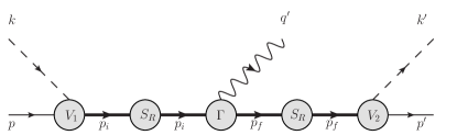
Figure 1: Resonant part of the process $\phi\,\psi\to\gamma\,\phi\,\psi$. The thick, thin, dashed, and wiggly lines correspond to the heavy fermion, the light fermion, the neutral pseudoscalar, and the photon, respectively.

Our aim is to investigate the charge and the magnetic moment of the heavy fermion. As this fermion is an unstable ”particle” it cannot appear in an asymptotic state. Therefore, let us consider the amplitude of the process

$$\phi(k)+\psi(p)\to\gamma(q^{\prime})+\phi(k^{\prime})+\psi(p^{\prime})$$

for an invariant energy near the mass of the resonance (see Fig. 1). The total amplitude $A$ will be the sum of a resonant part $A_{\rm r}$ and a non-resonant part $A_{\rm n.r.}$. The resonant part can be written as

$$A_{\rm r} = -i\,e\,\epsilon_{\mu}^{\ast}\,V_{2}(p^{\prime},p_{f})iS_{R}(p_{f})\Gamma^{\mu}(p_{f},p_{i})iS_{R}(p_{i})V_{1}(p_{i},p)\,,$$ (4)

where $\epsilon$ denotes the polarization vector of the photon, and $p_{i}=p+k$ and $p_{f}=p^{\prime}+k^{\prime}$ refer to the intermediate resonance momenta before and after the electromagnetic interaction, respectively. The dressed propagator of the heavy fermion $S_{R}$ reads

$$S_{R}(p)=\frac{1}{p/\hskip 1.00006pt-M_{R}-\Sigma(p/\hskip 1.00006pt)}\,,$$ (5)

where $-i\Sigma(p/\hskip 1.00006pt)$ is the sum of the one-particle-irreducible diagrams contributing to the two-point function of the heavy fermion.

The dressed propagator $S_{R}$ has a complex pole which is obtained by solving the equation

$$z-M_{R}-\Sigma(z)=0\,.$$ (6)

We define the pole mass as the real part of $z$. In the vicinity of the pole, $S_{R}$ can be written as

$$S_{R}(p)=\frac{Z}{p/\hskip 1.00006pt-z}+{\rm n.p.}=\frac{Z\left(p/\hskip 1.00006pt+z\right)}{p^{2}-z^{2}}+{\rm n.p.}\,,$$ (7)

where n.p. generically denotes non-pole, i.e. regular terms. The residue $Z$ is given by

$$Z=1+\delta Z=\frac{1}{1-\Sigma^{\prime}(z)}\,.$$ (8)

For purely technical convenience in the calculations to follow, let us introduce “Dirac spinors” with complex masses $z$,

$$w^{1}(p) \equiv \sqrt{p_{0}+z}\left(\begin{array}[]{c}1\\ 0\\ \frac{p_{z}}{p_{0}+z}\\ \frac{p_{x}+ip_{y}}{p_{0}+z}\end{array}\right)\,,$$ (13)

$$\bar{w}^{1}(p) \equiv \sqrt{p_{0}+z}\left(\begin{array}[]{llll}1\,,&0\,,&\frac{-p_{z}}{p_{0}+z}\,,&-\frac{p_{x}-ip_{y}}{p_{0}+z}\end{array}\right),$$ (15)

$$w^{2}(p) \equiv \sqrt{p_{0}+z}\left(\begin{array}[]{c}0\\ 1\\ \frac{p_{x}-ip_{y}}{p_{0}+z}\\ \frac{-p_{z}}{p_{0}+z}\end{array}\right)\,,$$ (20)

$$\bar{w}^{2}(p) \equiv \sqrt{p_{0}+z}\left(\begin{array}[]{llll}0\,,&1\,,&-\frac{p_{x}+ip_{y}}{p_{0}+z}\,,&\frac{p_{z}}{p_{0}+z}\end{array}\right).$$ (22)

For $p^{2}=z^{2}$, the spinors satisfy the “Dirac equations”

$$\left(p/\hskip 1.00006pt-z\right)w^{i} = 0\,,$$

$$\bar{w}^{i}\left(p/\hskip 1.00006pt-z\right) = 0$$ (23)

as well as the identity

$$w^{i}(p)\,\bar{w}^{i}(p)=p/\hskip 1.00006pt+z\,,$$ (24)

where a summation over $i=1,2$ is implied. For $p^{2}\neq z^{2}$, the difference between $w^{i}(p)\,\bar{w}^{i}(p)$ and $p/\hskip 1.00006pt+z$ is of ${\cal O}(p^{2}-z^{2})$ so that we can write for the dressed propagator

$$S_{R}(p)=\frac{Z\,w^{i}(p)\,\bar{w}^{i}(p)}{p^{2}-z^{2}}+{\rm n.p.}\,.$$ (25)

Substituting Eq. (25) in Eq. (4) we decompose the resonant amplitude in a double-pole contribution $A_{\rm d.p.}$ and the rest Sirlin:1991fd , where

$$A_{\rm d.p.} = -i\,e\,\epsilon_{\mu}^{\ast}\,V_{2}(p^{\prime},p_{f})w^{i}(p_{f})\sqrt{Z}\frac{i}{p_{f}^{2}-z^{2}}$$ (26)

$$\times\sqrt{Z}\,\bar{w}^{i}(p_{f})\Gamma^{\mu}(p_{f},p_{i})w^{j}(p_{i})\sqrt{Z}$$

$$\times\frac{i}{p_{i}^{2}-z^{2}}\sqrt{Z}\bar{w}^{j}(p_{i})V_{1}(p_{i},p)\,.$$

Using Eqs. (23), we parameterize the renormalized vertex function for $p_{f}^{2}=p_{i}^{2}=z^{2}$ in terms of two form factors,

$$\sqrt{Z}\,\bar{w}^{i}(p_{f})\Gamma^{\mu}(p_{f},p_{i})w^{j}(p_{i})\sqrt{Z}=\bar{w}^{i}(p_{f})\left[\,\gamma^{\mu}\,F_{1}(q^{2})+i\,\sigma^{\mu\nu}\,q_{\nu}\,F_{2}(q^{2})\,\right]w^{j}(p_{i})\,,$$ (27)

where $q=p_{f}-p_{i}$. Note that our normalization of $F_{2}$ differs by a constant factor from the one commonly used for stable particles.

III Form factors

Figure 2: One-loop self-energy diagram of the heavy fermion. The thick, thin, and dashed lines correspond to the heavy fermion, the light fermion, and the neutral pseudoscalar, respectively.

Below, we calculate the form factors $F_{1}$ and $F_{2}$ to one-loop order at $q^{2}=0$. For that purpose we need to obtain the one-loop contributions to the wave function renormalization constant $Z$ and the vertex function $\Gamma^{\mu}$ at $q^{2}=0$. The one-loop contribution to the heavy-fermion self-energy generated by the interaction terms explicitly given in Eqs. (1) and (3) is shown in Fig. 2. We obtain for $\delta Z$ of the residue $Z=1+\delta Z$ of Eq. (8),

$$\delta Z=g^{2}\delta Z_{a}+g\xi\delta Z_{b}\,,$$ (28)

where the explicit expressions for the coefficients $\delta Z_{a}$ and $\delta Z_{b}$ are given in Eqs. (41) and (42) in the appendix. The contribution of the tree-order vertex diagram to $\Gamma^{\mu}$ reads

$$\Gamma_{\rm tree}^{\mu}=\gamma^{\mu}+2\kappa\,i\,\sigma^{\mu\nu}\,q_{\nu}\,.$$ (29)

The one-loop-order vertex diagrams generated by the interaction terms of Eqs. (1) and (3) are shown in Fig. 3.

Figure 3: One-loop diagrams contributing to the photon heavy-fermion vertex function. The thick, thin, dashed, and wiggly lines correspond to the heavy fermion, the light fermion, the neutral pseudoscalar, and the photon, respectively.

For $q^{2}=0$, the results of the diagrams in Figs. 3 (a) and (b) read, respectively,

$$\Gamma^{\mu}_{a} = g^{2}\left(\gamma^{\mu}\,f_{1a}+i\,\sigma^{\mu\nu}\,q_{\nu}\,f_{2a}\right),$$

$$\Gamma^{\mu}_{b} = g\xi\left(\gamma^{\mu}\,f_{1b}+i\,\sigma^{\mu\nu}\,q_{\nu}\,f_{2b}\right).$$ (30)

For the coefficients we obtain

$$f_{1a} = -\delta Z_{a},$$

$$f_{1b} = -\delta Z_{b},$$

$$f_{2b} = -2\kappa\delta Z_{b},$$

and the expression for $f_{2a}$ is given in Eq. (43) in the appendix. Putting the results together, the form factors at $q^{2}=0$ are given by

$$F_{1}(0) = 1\,,$$

$$F_{2}(0) = 2\kappa+g^{2}(2\kappa\delta Z_{a}+f_{2a})$$ (31)

$$= 2\kappa+\frac{g^{2}}{32\pi^{2}M_{R}\left(M_{R}^{2}+2M_{R}M_{N}+M_{N}^{2}-M^{2}\right)}[{\cal A}+{\cal B}+{\cal C}+{\cal D}]\,,$$

where

$${\cal A} = -(1-4\kappa M_{R})M^{2}_{R}-2M_{R}M_{N}-(1+4\kappa M_{R})(M^{2}_{N}+M^{2})\,,$$

$${\cal B} = \frac{2A_{0}\left(M^{2}\right)}{M_{R}^{2}}\left[3\kappa M_{R}^{3}+(1+2\kappa M_{R})M_{R}M_{N}+(1+3\kappa M_{R})(M_{N}^{2}-M^{2})\right],$$

$${\cal C} = \frac{2A_{0}\left(M^{2}_{N}\right)}{M_{R}^{2}}\left[\frac{M_{R}^{3}}{M_{N}}+(1+\kappa M_{R})M_{R}^{2}-(1+2\kappa M_{R})M_{R}M_{N}-(1+3\kappa M_{R})(M_{N}^{2}-M^{2})\right],$$

$${\cal D} = -\frac{2B_{0}\left(M_{R}^{2},M^{2},M_{N}^{2}\right)}{M_{R}^{2}}\left[\kappa M_{R}^{5}+(1+2\kappa M_{R})M_{R}M_{N}(M_{R}^{2}+M_{R}M_{N}-M_{N}^{2}+M^{2})\right.$$ (32)

$$\quad\quad\quad\quad\quad\quad\quad\quad\quad\quad\left.+2\kappa M_{R}^{3}M^{2}-(1+3\kappa M_{R})(M_{N}^{2}-M^{2})^{2}\right].$$

As expected the charge does not get renormalized, i.e. $F_{1}(0)=1$. Moreover, the magnetic moment does not depend on the field-redefinition parameter $\xi$. This is the case, because in both charge and magnetic moment the $\xi$-dependent part of the residue of the propagator exactly cancels the $\xi$-dependent parts of the loop vertex diagrams of Fig. 3 (b). For an unstable heavy fermion ($M_{R}>M_{N}+M$), the latter also contain imaginary parts. Therefore, any alternative definition of the charge and the magnetic moment, making use of a real-valued wave function renormalization constant, necessarily leads to $\xi$-dependent and thus unphysical quantities. For example, let us denote by $M_{R}^{R}$ the mass of the heavy fermion defined as the zero of the real part of the inverse propagator, i.e.

$$M_{R}^{R}-M_{R}-{\rm Re}\,\Sigma(M_{R}^{R})=0\,.$$ (33)

In Refs. Sirlin:1991fd ; Sirlin:1991rt ; Willenbrock:1991hu ; Gegelia:1992kj ; Gambino:1999ai ; Djukanovic:2007bw it was shown that this definition leads to gauge- and field-redefinition-parameter-dependent masses of the unstable particles starting at two-loop order. Even though from a phenomenological point of view one might argue that a deviation at the two-loop level is small, as a matter of principle, a physical quantity by definition should be gauge and field-redefinition independent. Moreover, as we will see below, we encounter similar problems already at one-loop order and there is no good reason to ignore this issue.

Close to $p/\hskip 1.00006pt\sim M_{R}^{R}$, the dressed propagator can be written as

$$S_{R}(p) = \frac{1}{\left(p/\hskip 1.00006pt-M_{R}^{R}\right)\left[1-\Sigma^{\prime}(M_{R}^{R})\right]-i\,{\rm Im}\,\Sigma(M_{R}^{R})+{\cal O}\left[\left(p/\hskip 1.00006pt-M_{R}^{R}\right)^{2}\right]}$$ (34)

$$= \frac{Z_{R}}{\left(p/\hskip 1.00006pt-M_{R}^{R}\right)\left[1-iZ_{R}\,{\rm Im}\,\Sigma^{\prime}(M_{R}^{R})\right]-i\,Z_{R}\,{\rm Im}\,\Sigma(M_{R}^{R})+{\cal O}\left[\left(p/\hskip 1.00006pt-M_{R}^{R}\right)^{2}\right]}\,,$$

where

$$Z_{R}=\frac{1}{1-{\rm Re}\,\Sigma^{\prime}(M_{R}^{R})}\,.$$

Up to one-loop accuracy Eq. (34) can be written as

$$S_{R}(p) = \frac{Z_{R}}{\left(p/\hskip 1.00006pt-M_{R}^{R}\right)\left[1-i\,{\rm Im}\,\Sigma^{\prime}(M_{R}^{R})\right]-i\,{\rm Im}\,\Sigma(M_{R}^{R})+{\cal O}\left[\left(p/\hskip 1.00006pt-M_{R}^{R}\right)^{2}\right]}\,$$ (35)

with

$$Z_{R}=1+{\rm Re}\,\Sigma^{\prime}(M_{R}^{R})\,.$$

Expanding the fraction and keeping only terms up to one-loop accuracy, we obtain

$$S_{R}(p)=Z_{R}\frac{p/\hskip 1.00006pt+M_{R}^{R}+i\,{\rm Im}\,\Sigma(M_{R}^{R})}{p^{2}-{M_{R}^{R}}^{2}+iM_{R}^{R}\,\Gamma_{R}(p^{2})}$$

which has the characteristic Breit-Wigner form with an energy-dependent width

$$\Gamma_{R}(p^{2})=-2\,{\rm Im}\,\Sigma(M_{R}^{R})-\left(p^{2}-{M_{R}^{R}}^{2}\right)\frac{{\rm Im}\,\Sigma^{\prime}(M_{R}^{R})}{M_{R}^{R}},$$

and a real wave function renormalization constant $Z_{R}$ Sirlin:1991fd .

Using the Dirac spinors of Eqs. (22) with the mass $M_{R}^{R}$ instead of a complex $z$, putting the external legs of the vertex functions ”on mass shell”, i.e. $p/\hskip 1.00006pt=M_{R}^{R}$, and taking $Z_{R}$ as the wave function renormalization constant, we obtain for the form factors the following results:

$$F_{1}(0) = 1+\frac{i\,g^{2}\,{\rm Im}\left[B_{0}\left(M_{R}^{2},M^{2},M_{N}^{2}\right)\right]}{32\pi^{2}M_{R}^{2}\left(M_{R}^{2}+2M_{R}M_{N}+M_{N}^{2}-M^{2}\right)}\biggl{[}M_{R}^{4}+2M_{R}^{3}M_{N}$$

$$+2M_{R}^{2}\left(M_{N}^{2}+M^{2}\right)-2M_{R}M_{N}\left(M_{N}^{2}-M^{2}\right)-3\left(M_{N}^{2}-M^{2}\right)^{2}\biggr{]}$$

$$-\frac{i\,g\,\xi\,{\rm Im}\left[B_{0}\left(M_{R}^{2},M^{2},M_{N}^{2}\right)\right]\left[M_{R}^{4}-2M_{R}^{2}\left(M_{N}^{2}+M^{2}\right)+\left(M_{N}^{2}-M^{2}\right)^{2}\right]}{16\pi^{2}M_{R}\left(M_{R}^{2}+2M_{R}M_{N}+M_{N}^{2}-M^{2}\right)}\,,$$

$$F_{2}(0) = 2\,\kappa+\frac{g^{2}}{32\pi^{2}M_{R}\left(M_{R}^{2}+2M_{R}M_{N}+M_{N}^{2}-M^{2}\right)}\,({\cal A}+{\cal B}+{\cal C}+{\cal D}_{1}+\mbox{Re}[{\cal D}_{2}])$$ (36)

$$-\frac{i\,g\,\xi\,\kappa\,{\rm Im}\left[B_{0}\left(M_{R}^{2},M^{2},M_{N}^{2}\right)\right]\left(M_{R}^{2}-2M_{R}M_{N}+M_{N}^{2}-M^{2}\right)}{8\pi^{2}M_{R}}\,,$$

where ${\cal A}$, ${\cal B}$, ${\cal C}$, and ${\cal D}$ are given in Eqs. (III), and ${\cal D}_{1}$ and ${\cal D}_{2}$ refer to the $\kappa$-independent and $\kappa$-dependent parts of ${\cal D}$, respectively. From Eqs. (36) it is clearly seen that within the “on-mass-shell” scheme the charge of the unstable heavy fermion receives “strong” corrections. Furthermore, both the charge and the magnetic moment have imaginary parts which depend on the field-redefinition parameter $\xi$. Such a definition does not qualify as a physical observable.

One might define the vertex function using Eq. (27) with a Breit-Wigner mass $M_{R}^{R}$ instead of $z$, in combination with the complex wave function renormalization constant

$$Z=\frac{1}{1-\Sigma^{\prime}(M_{R}^{R})}\,.$$

At one-loop order such a definition leads to the non-renormalization of the charge and a $\xi$-independent magnetic moment. This is the case because the so obtained one-loop-order result coincides with the one extracted at the pole position. Now the problem shows up starting at two-loop order.

Let us analyze the $\xi$ dependence at two-loop order. For simplicity we take $\kappa=0$ and consider the vertex function at $q^{2}=0$ and $p_{i}^{2}=p_{f}^{2}=z^{2}$ with $z$ corresponding to either the pole or to the Breit-Wigner mass,

$$G^{\mu,ij}(p_{f},p_{i})=Z(z)\,\bar{w}^{i}(p_{f})\Gamma^{\mu}(p_{f},p_{i})w^{j}(p_{i})=Z(z)\,\bar{w}^{i}(p_{f})\left[\,\gamma^{\mu}\,W_{1}(z)+i\,\sigma^{\mu\nu}\,q_{\nu}\,W_{2}(z)\,\right]w^{j}(p_{i})\,,$$ (37)

where

$$Z(z)=\frac{1}{1-\Sigma^{\prime}(z)}=1+\hbar\,\delta Z^{(1)}(z)+\hbar^{2}\,\delta Z^{(2)}(z)+{\cal O}(\hbar^{3})\,.$$ (38)

In Eq. (38), the expansion in $\hbar$ corresponds to the loop expansion. The Ward identity guarantees that

$$Z(z)\,W_{1}(z)=1,$$ (39)

and therefore the charge is not renormalized. Expanding $W_{2}(z)$ in the number of loops,

$$W_{2}(z)=\hbar\,W_{2}^{(1)}(z)+\hbar^{2}\,W_{2}^{(2)}(z)+{\cal O}(\hbar^{3})\,,\\$$

and substituting Eq. (38) and $z=M_{R}+\hbar\,\delta M+{\cal O}(\hbar^{2})$ into Eq. (37), we obtain for the vertex function up to and including order $\hbar^{2}$,

$$G^{\mu,ij}(p_{f},p_{i}) = \bar{w}^{i}(p_{f})\biggl{(}\gamma^{\mu}+i\,\sigma^{\mu\nu}\,q_{\nu}\,\biggl{\{}\hbar W_{2}^{(1)}(M_{R})$$ (40)

$$+\hbar^{2}\,\left[W_{2}^{(2)}(M_{R})+\delta Z_{1}(M_{R})W_{2}^{(1)}(M_{R})+\delta M\,W_{2}^{(1)^{\prime}}(M_{R})\right]\biggr{\}}\,\biggr{)}w^{j}(p_{i})\,,$$

where

$$W_{2}^{(1)^{\prime}}(M_{R})=\left.\frac{dW_{2}^{(1)}(z)}{dz}\right|_{z=M_{R}}.$$

At order $\hbar$, the vertex function is independent of $\xi$ for any choice of $\delta M$, because $W_{2}^{(1)}(M_{R})$ does not depend on $\xi$. At order $\hbar^{2}$, for this to happen the $\xi$-dependent parts of $W_{2}^{(2)}(M_{R})$ and of the remaining two terms have to precisely cancel each other. The calculated result for $W_{2}^{(1)^{\prime}}(M_{R})$ contains a non-vanishing term linear in $\xi$. For $z$ chosen as the pole position of the dressed propagator this cancelation has to take place as the residue of the $S$-matrix cannot depend on $\xi$. For any other choice of $z$ (i.e. $\delta M$), including the Breit-Wigner mass, a $\xi$ dependence remains at two-loop order. We therefore conclude that the physical quantities characterizing the unstable particles should be defined at the complex pole of the dressed propagator, because only this specification guarantees a $\xi$-independent result at arbitrary loop order.

IV Summary

In the framework of effective quantum field theory we have addressed the definition of physical quantities characterizing unstable particles. To that end we considered a charged, unstable heavy fermion which we allowed to decay into a charged, stable light fermion and a stable, neutral pseudoscalar. While our arguments are applicable to all physical quantities characterizing unstable particles, we have focussed on the charge and the magnetic moment of the resonance. Our discussion made use of the well-known fact that observables should remain invariant under a field transformation. With this in mind, we performed in our model Lagrangian a particular field transformation depending on an arbitrary parameter $\xi$. By appealing to the $\xi$ independence of physical quantities, in a one-loop calculation we demonstrated that physical properties characterizing unstable resonances should be defined through the residues of the $S$-matrix in the complex plane. As opposed to this, if the ”on-mass-shell” scheme is used then even the charge and not only the magnetic moment will receive contributions from the strong interactions and both will depend on the parameter $\xi$. In summary, the main conclusion is that physical quantities characterizing unstable particles should be extracted from the residues at complex poles. This observation neither depends on the choice of observables nor on the details specific to the model.

V Appendix

In the following we collect the contributions of the loop diagrams of Figs. 2 and 3 to the wave function renormalization constant and the vertex functions, respectively. The loop functions $A_{0}$ and $B_{0}$ are defined as

$$A_{0}(m^{2}) = \frac{(2\pi)^{4-n}}{i\,\pi^{2}}\,\int\frac{d^{n}k}{k^{2}-m^{2}+i\,0^{+}}\,,$$

$$B_{0}(p^{2},m_{1}^{2},m_{2}^{2}) = \frac{(2\pi)^{4-n}}{i\,\pi^{2}}\,\int\frac{d^{n}k}{\left[k^{2}-m_{1}^{2}+i\,0^{+}\right]\left[(p+k)^{2}-m_{2}^{2}+i\,0^{+}\right]}\,.$$

The coefficients $\delta Z_{a}$ and $\delta Z_{b}$ of Eq. (28) are given by

$$\delta Z_{a} = \frac{M_{R}^{2}-M_{N}^{2}-M^{2}}{16\pi^{2}\left(M_{R}^{2}+2M_{R}M_{N}+M_{N}^{2}-M^{2}\right)}$$ (41)

$$+\frac{\left(3M_{R}^{2}+2M_{R}M_{N}+3M_{N}^{2}-3M^{2}\right)A_{0}\left(M^{2}\right)}{32\pi^{2}M_{R}^{2}\left(M_{R}^{2}+2M_{R}M_{N}+M_{N}^{2}-M^{2}\right)}$$

$$+\frac{\left(M_{R}^{2}-2M_{R}M_{N}-3M_{N}^{2}+3M^{2}\right)A_{0}\left(M_{N}^{2}\right)}{32\pi^{2}M_{R}^{2}\left(M_{R}^{2}+2M_{R}M_{N}+M_{N}^{2}-M^{2}\right)}$$

$$-\frac{B_{0}\left(M_{R}^{2},M^{2},M_{N}^{2}\right)}{32\pi^{2}M_{R}^{2}\left(M_{R}^{2}+2M_{R}M_{N}+M_{N}^{2}-M^{2}\right)}$$

$$\times\biggl{[}M_{R}^{4}+2M_{R}^{3}M_{N}+2M_{R}^{2}M_{N}^{2}+2M_{R}^{2}M^{2}-2M_{R}M_{N}^{3}$$

$$\,\,\,\,\,\,\,+2M_{R}M_{N}M^{2}-3M_{N}^{4}+6M_{N}^{2}M^{2}-3M^{4}\biggr{]}$$

and

$$\delta Z_{b}=\frac{1}{16\pi^{2}M_{R}}\biggl{\{}A_{0}\left(M^{2}\right)-A_{0}\left(M_{N}^{2}\right)+\biggl{[}M_{R}^{2}+M_{N}^{2}-2M_{R}M_{N}-M^{2}\biggr{]}B_{0}\left(M_{R}^{2},M^{2},M_{N}^{2}\right)\biggr{\}}\,.$$ (42)

The coefficients $f_{1a}$, $f_{2a}$, $f_{1b}$, and $f_{2b}$ of Eqs. (III) are given by

$$f_{1a} = -\delta Z_{a},$$

$$f_{2a} = \frac{1}{32\pi^{2}M_{R}^{3}M_{N}\left(M_{R}^{2}+2M_{R}M_{N}+M_{N}^{2}-M^{2}\right)}$$ (43)

$$\times\biggl{\{}-M_{R}^{2}M_{N}\left(M_{R}^{2}+2M_{R}M_{N}+M_{N}^{2}+M^{2}\right)$$

$$\,\,\,\,\,\,\,\,\,+2M_{N}\left(M_{R}M_{N}+M_{N}^{2}-M^{2}\right)A_{0}\left(M^{2}\right)$$

$$\,\,\,\,\,\,\,\,\,+2\left(M_{R}^{3}+M_{R}^{2}M_{N}-M_{R}M_{N}^{2}-M_{N}^{3}+M_{N}M^{2}\right)A_{0}\left(M_{N}^{2}\right)$$

$$\,\,\,\,\,\,\,\,\,-2M_{N}\left(M_{R}^{3}M_{N}+M_{R}^{2}M_{N}^{2}-M_{R}M_{N}^{3}+M_{R}M_{N}M^{2}-M_{N}^{4}+2M_{N}^{2}M^{2}-M^{4}\right)$$

$$\,\,\,\,\,\,\,\,\,\times B_{0}\left(M_{R}^{2},M^{2},M_{N}^{2}\right)\biggr{\}}\,,$$

$$f_{1b} = -\delta Z_{b},$$

$$f_{2b} = -2\kappa\delta Z_{b}.$$

References

• (1) P. T. Matthews and A. Salam, Phys. Rev.  112, 283 (1958).
• (2) P. T. Matthews and A. Salam, Phys. Rev.  115, 1079 (1959).
• (3) R. Jacob and R. G. Sachs, Phys. Rev.  121, 350 (1961).
• (4) S. Willenbrock and G. Valencia, Phys. Lett.  B 247, 341 (1990).
• (5) G. Valencia and S. Willenbrock, Phys. Rev.  D 42, 853 (1990).
• (6) A. Sirlin, Phys. Rev. Lett.  67, 2127 (1991).
• (7) A. Sirlin, Phys. Lett.  B 267, 240 (1991).
• (8) S. Willenbrock and G. Valencia, Phys. Lett.  B 259, 373 (1991).
• (9) J. Gegelia, G. Japaridze, A. Tkabladze, A. Khelashvili and K. Turashvili, in Proceedings of the International Seminar on Quarks (Quarks ’92), Zvenigorod, Russia, 1992, edited by D. Yu. Grigoriev, V. A. Matveev, V. A. Rubakov, and P. G. Tinyakov (World Scientific, Singapore, 1993).
• (10) P. Gambino and P. A. Grassi, Phys. Rev.  D 62, 076002 (2000).
• (11) G. ’t Hooft and M. J. G. Veltman, Nucl. Phys.  B50, 318 (1972).
• (12) B. W. Lee and J. Zinn-Justin, Phys. Rev.  D 5, 3121 (1972).
• (13) D. Gross, in Methods In Field Theory, edited by R. Balian and J. Zinn-Justin (North-Holland, Amsterdam, 1976).
• (14) H. Wittig, in Landolt-Börnstein - Group I Elementary Particles, Nuclei and Atoms, Volume 21 A: Elementary Particles (Springer, Berlin, 2008).
• (15) C. Alexandrou et al., Phys. Rev.  D 79, 014507 (2009).
• (16) V. M. Braun et al., Phys. Rev. Lett.  103, 072001 (2009).
• (17) S. Boinepalli, D. B. Leinweber, P. J. Moran, A. G. Williams, J. M. Zanotti, and J. B. Zhang, arXiv:0902.4046 [hep-lat].
• (18) S. Weinberg, Physica A96, 327 (1979).
• (19) J. Gasser and H. Leutwyler, Annals Phys.  158, 142 (1984).
• (20) J. Gasser, M. E. Sainio, and A. Švarc, Nucl. Phys. B307, 779 (1988).
• (21) S. Scherer, Adv. Nucl. Phys.  27, 277 (2003).
• (22) V. Pascalutsa, M. Vanderhaeghen, and S. N. Yang, Phys. Rept.  437, 125 (2007).
• (23) S. Scherer, Prog. Part. Nucl. Phys. (2009), doi:10.1016/j.ppnp.2009.08.002.
• (24) L. Tiator, D. Drechsel, S. Kamalov, M. M. Giannini, E. Santopinto, and A. Vassallo, Eur. Phys. J.  A 19, 55 (2004).
• (25) V. D. Burkert and T. S. H. Lee, Int. J. Mod. Phys.  E 13, 1035 (2004).
• (26) S. Capstick et al., Eur. Phys. J.  A 35, 253 (2008).
• (27) V. D. Burkert, AIP Conf. Proc.  1056, 348 (2008).
• (28) M. Kotulla, Prog. Part. Nucl. Phys.  61, 147 (2008).
• (29) S. Kamefuchi, L. O’Raifeartaigh, and A. Salam, Nucl. Phys.  28, 529 (1961).
• (30) S. R. Coleman, J. Wess, and B. Zumino, Phys. Rev.  177, 2239 (1969).
• (31) S. Scherer and H. W. Fearing, Phys. Rev.  C 51, 359 (1995).
• (32) S. Weinberg, The Quantum Theory of Fields, Vol. 1: Foundations (Cambridge University Press, Cambridge, England, 1995), Chap. 7.7.
• (33) H. W. Fearing and S. Scherer, Phys. Rev.  C 62, 034003 (2000).
• (34) D. Djukanovic, J. Gegelia, and S. Scherer, Phys. Rev.  D 76, 037501 (2007).