Mean-field methods in evolutionary duplication-innovation-loss models for the genome-level repertoire of protein domains

Abstract

We present a combined mean-field and simulation approach to different models describing the dynamics of classes formed by elements that can appear, disappear or copy themselves. These models, related to a paradigm duplication-innovation model known as Chinese Restaurant Process, are devised to reproduce the scaling behavior observed in the genome-wide repertoire of protein domains of all known species. In view of these data, we discuss the qualitative and quantitative differences of the alternative model formulations, focusing in particular on the roles of element loss and of the specificity of empirical domain classes.

I Introduction

Understanding the complexity of genomes and the drives that shape them is a fundamental problem of contemporary biology Tautz and Lassig (2004), which poses a number of challenges to contemporary statistical mechanics. Considering this problem from a large-scale viewpoint, the basic observables to account for are the distributions of the different “functional components” (such as genes, introns, non-coding RNA, etc.) encoded by sequenced genomes of varying size.

When these genome-wide data are parametrized by measures of “genome size” (such as the number of bases or the number of genes in a genome), there are important emerging “scaling laws” both for the classes of evolutionary related genes Huynen and van Nimwegen (1998); Mattick (2004); Maslov et al. (2009), the functional categories of genes van Nimwegen (2003); Itzkovitz et al. (2006) and some non-coding parts of genomes Lynch and Conery (2003). These scaling laws are the signs of universal invariants in the processes and constraints that gave rise to the genomes as they can be observed today. A current challenge is the understanding of these laws using physical modeling concepts and the comparison of the models to the available whole-genome data. This effort can help disentangle neutral from selective effects Rocha (2008); Koonin (2009).

Here we consider the statistical features of the set of proteins expressed by a genome, or proteome. A convenient level of analysis is a description of the proteome in terms of structural protein domains Orengo and Thornton (2005). Domains are modular “topologies”, or sub-shapes, forming proteins Branden and Tooze (1999). A domain determines a set of potential biochemical or biophysical functions and interactions for a protein, such as binding to other proteins or DNA and participation in well-defined classes of biochemical reactions Orengo and Thornton (2005); Itzkovitz et al. (2006). Despite the practically unlimited number of possible protein sequences, the repertoire of basic topologies for domains seems to be relatively small Koonin et al. (2002). With a loose parallel, domains could be seen as an “alphabet” of basic elements of the protein universe. Understanding the usage of domains across organisms is as important and challenging as decoding an unknown language.

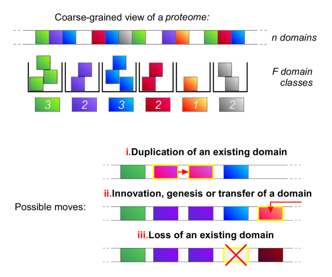
The content of a genome is determined primarily by its evolutionary history, in which neutral processes and natural selection play interdependent roles. In particular, the coding parts of genomes evolve by some well-defined basic “moves”: gene loss, gene duplication, horizontal gene transfer (the transfer of genetic material between unrelated species), and gene genesis (the de novo origin of genes). Since domains are modular evolutionary building blocks for proteins, they are coupled to the dynamics followed by genes. In particular, a new domain topology can emerge by genesis or horizontal transfer, and new domains of existing domain topologies can emerge by duplication or be lost. Finally, topologies can be completely lost by a genome if the last domain that carries them is lost (see Fig. 1).

Large-scale data concerning structural domains are available from bioinformatic databases, and can be analyzed at the genome level. These coarse-grained data structures can be represented as sets of “domain classes” (the sets of all realizations of the same domain topology in proteins), populated by domain realizations. In particular, much attention has been drawn by the intriguing discovery that the population of domain classes have power-law distributions Qian et al. (2001); Karev et al. (2002); Kuznetsov (2002); Abeln and Deane (2005); Dokholyan et al. (2002): the number $F(j,n)$ of domain classes having $j$ members follows the power-law $\sim 1/j^{z}$, where the exponent $z$ typically lies between 1 and 2. An interesting thread of modeling work ascribes the emergence of power-laws to a generic preferential-attachment principle due to gene duplication. Growth models are formulated as nonstationary, duplication-innovation models Qian et al. (2001); Kamal et al. (2006); Durrett and Schweinsberg (2005) and as stationary birth-death-innovation models Karev et al. (2002, 2003, 2004, 2005).

Intriguingly, as we have recently shown Cosentino Lagomarsino et al. (2009), the domain content of genomes also exhibits scaling laws as a function of the total number of domains $n$, indicating that even evolutionarily distant genomes show common trends where the relevant parameter is their size.

• The number of domain classes (or distinct hits of the same domain) concentrates around a master curve $F(n)$ that appears to be markedly sublinear with size, perhaps saturating.

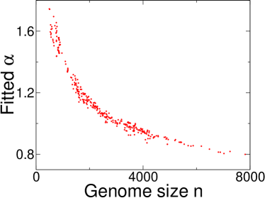
• The fitted exponent of the power-law-like distribution $F(j,n)$ of domain classes having $j$ members, in a proteome of size $n$ decreases with genome size. In other words, there is evidence for a cutoff that increases linearly with $n$.

• The occurrence of fold topologies across genomes is highly inhomogeneous - some domain superfamilies are found in all genomes, some rare, with a sigmoid-like drop between these two categories .

We recently reported the above collective trends, and showed how the scaling laws in the data could be reproduced using universal parameters with non-stationary duplication-innovation models. Our results indicate that the basic evolutionary moves themselves can determine the observed scaling behavior of domain content, a priori of more specific biological trends.

This modeling approach, while similar in formulation to that of previous investigators Qian et al. (2001) who did not consider these scaling laws, has important modifications, mostly related to the scaling with $n$ of the relative probability of adding a domain belonging to a new class and duplicating an existing one. To reproduce the observed trends, newly added domain classes cannot be treated as independent random variables, but are conditioned by the preexisting proteome structure.

In this paper, we give a detailed account of this modeling approach, considering different variants of duplication-innovation-loss models for protein domains, and relate them to available results in the mathematical and physical literature. In particular, we will focus on mean-field approaches for the models and comparison with direct simulation, and we will show how they can be generally used to obtain the main qualitative and quantitative trends.

The first part of the paper is devoted to the minimal model formulation, which only includes duplication and innovation moves for domains, and relates to the so-called Chinese Restaurant Process (CRP) of the mathematical literature Pitman (2002); Pitman and Yor (1997). We will review the main known results for this model, derive analytically solvable mean-field equations, and show how they compare to the available rigorous results and the finite size behavior.

The rest of the paper is devoted to biologically motivated variants of the main model related to two main features: including the role of loss of domains, which is a frequently reported event, and breaking the exchange symmetry of domain classes, which is unrealistic, as specific protein domains perform different biological functions. For these variants, we will present mean-field and simulations results, and characterize their phenomenology in relation with empirical data. In particular, while in general for these variants the rigorous mathematical results existing for the CRP break down, we will show how the use of simple mean-field methods proves to be a robust tool for accessing the qualitative phenomenology.

II Generic features of the model

The model represents a proteome through its repertoire of domains. Domains having the same topology are collected in domain classes (Fig. 1). Thus the relevant data structures are partitions of elements (domains) into classes. The basic observables considered are the following: $n$, the total number of domains, $f(n)$, a random variable indicating the number of classes (distinct domain topologies) at size $n$, a random variable $k_{i}$, the population of class $i$, $n_{i}$, the size at birth of class $i$, and $f(j,n)$: the number of domain classes having $j$ members. We will generally indicate mean values by capitalized letters (e.g. $F(n)$ is the mean value of $f(n)$, $K_{i}$ the mean value of $k_{i}$, etc.).

The model is conceived as a stochastic process based on the elementary moves available to a genome (Fig. 1) of adding and losing domains, associated to relative probabilities: $p_{O}$, the probability to duplicate an old domain (modeling gene duplication), $p_{N}$, the probability to add a new domain class with one member (which describes domain innovation, for example by horizontal transfer), and $p_{L}$, a loss probability (which we will initially disregard, and consider in a second step). Iteratively, either a domain is added or it is lost with the prescribed probabilities.

Figure 1: (Color online) Scheme of the generic features of the duplication-innovation-loss model. Top: The sequences of proteins coded by a genome can be broken down into domains, represented by colored boxes. All the boxes of the same color, representing domains with the same topology are collected in the same domain class. Bottom: basic moves. Elements of a class can be duplicated or lost, and new classes can be formed with prescribed probabilities.

An important feature of the duplication move is the (null) hypothesis that duplication of a domain has uniform probability along the genome, and thus it is more probable to pick a domain of a larger class. This is a common feature with previous models Qian et al. (2001). This hypothesis creates a “preferential attachment” Barabasi and Albert (1999) principle, stating the fact that duplication is more likely in a larger domain class, which, in this model as in previous ones, is responsible for the emergence of power-law distributions.

In mathematical terms, if the duplication probability is split as the sum of per-class probabilities $p_{O}^{i}$, this hypothesis requires that $p_{O}^{i}\propto k_{i}$, where $k_{i}$ is the population of class $i$, i.e. the probability of finding a domain of a particular class and duplicating it is proportional to the number of members of that class.

It is important to notice that in this model, while $n$ can be used as an arbitrary measure of time, the ratio of the time-scales of duplication and innovation is not arbitrary, and is set by the ratio $p_{N}/p_{O}$. In the model of Gerstein and coworkers, this is taken as a constant, as the innovation move considered to be statistically independent from the genome content. In particular, both probabilities are considered to be constant. This choice has two problems. First, it cannot give the observed sublinear scaling of $F(n)$. Indeed, if the probability of adding a new domain is constant with $n$, so will be the rate of addition, implying that this quantity will increase on average linearly with genome size. Moreover, the same model gives power-law distributions for the classes with exponent larger than two, in contrast with most of the available data.

Previous investigators did not consider the fact that genomes cluster around a common curve Cosentino Lagomarsino et al. (2009), and thought of each of them as coming from an independent stochastic process with different parameters Qian et al. (2001). Furthermore, choosing constant $p_{N}$ implies that for larger genomes the influx of new domain families is heavily dominant on the flux of duplicated domains.

As noted by Durrett and Schweinsberg Durrett and Schweinsberg (2005), constant $p_{N}$ makes sense only if one thinks that new fold topologies emerge from an internal “nucleation-like” process with constant rate, rather than from an external flux. This process could be pictured as the genesis of new topologies from sequence mutation. Empirically, while genesis events are reported Kunin and Ouzounis (2003) and must occur, it is clear that domain topologies are very stable, and the exploration of sequence space is not free, but conditioned by a number of additional important factors, including chromosomal position and expression patterns of genes, and their role in biological networks Pal et al. (2006). Moreover, in prokaryotes, it is known that a large contribution to the innovation of coding genomes is provided by horizontal gene transfer Kunin and Ouzounis (2003), the exchange of genetic material between species, which can be reasonably represented in a model as an external flux, as opposed to the internal nucleation process representing genesis.

For eukaryotes, horizontal gene transfer is less important, and there can be multiple relevant innovation processes including exonization, loss of exons, alternative start sites changing the protein. We have not attempted to model the detailed processes leading to innovation, and because of their higher complexity in eukaryotes, we prefer to compare the model to the prokaryote data set alone. However, we can point out that in principle the same model has good agreement with the set of prokaryotes and eukaryotes together Cosentino Lagomarsino et al. (2009). In eukaryotes, the change in number of classes with respect to size change is generally small, but seems to have a trend that ”glues” quite well with prokaryotes (and in particular, innovation decreases with size).

Motivated by the sublinear scaling of the number of domain classes, and taking into account in an effective way the role of processes that condition the addition of new domain topologies, we consider statistically dependent moves. On general grounds, if a genome is a complex system where sub-components interact in clusters and non-locally, domain topologies as well have to be coordinated with other parts of the system, so that it is reasonable that evolutionary moves are conditioned by what is already present, and that the actual number of domain topologies need not to be trivially an extensive quantity.

The simplest way to implement this choice is to concentrate on the innovation process. Let us consider the indicator $\xi(n)$, taking value $1$ if a new domain class is born at size $n$, and value $0$ otherwise. The number of classes at size $n$ will be $f(n)=\sum_{j\leq n}\xi(j)$. If the random variables $\xi(n)$ are independent and identically distributed, i.e. $p(\xi(n)=1)=p_{N}=$constant, $f(n)$ follows a Bernoulli distribution whose mean value is linear in $n$. Moreover, $\frac{f(n)}{n}$ will be increasingly concentrated with increasing $n$ on the deterministic value $p_{N}$. If vice versa the random variables $\xi(n)$ are statistically dependent or also simply not identically distributed, the mean value may not be linear in $n$, and the concentration phenomenon may not occur. Both features, dependence and lack of concentration, are important. The former is necessary to obtain the observed sublinear behavior, the latter might create an intrinsic “diversity” in the genome ensemble, independently on the finite size of observed genomes (however, the currently available data are insufficient to establish this empirically).

III Simplest formulation: Chinese Restaurant Process

We investigate this process using analytical asymptotic equations and simulations. We start by considering only growth moves, by duplication and innovation, postponing the inclusion of domain loss in the model. We will see that the resulting model contains the basic qualitative phenomenology of the scaling laws and can thus be regarded as the paradigmatic case. One can arrive at the defining equations with different arguments. A simple way is to assume that domain duplication is a rare event, described by a Poisson distribution with characteristic time $\tau$, during which there is a flux of external or new domain topologies $\frac{\theta}{\tau}$. Then $p_{N}=\frac{\theta}{n+\theta}$. In this case the variables $\xi(n)$ are independent but not identically distributed. It is immediate to verify that $f(n)$ has mean value given by $\sum_{j=1}^{n}\frac{\theta}{\theta+j}$ and thus grows as $\sim\theta\log n$. The same result can be obtained by thinking of domain addition as a dependent move, conditioned on $n$, $f(n)$ or both.

It is possible to consider different intermediate scenarios where the pool of old domain classes is in competition with the universe explorable by the new classes. The simplest scheme, which turns out to be quite general, can be obtained by choosing the conditional probability that a new class is born $(\xi(n+1)=1)$ given the fact that $f(n)=f$ at size $n$

$$p_{N}=\frac{\theta+\alpha f}{n+\theta}\ \ ,$$ (1)

hence

$$p_{O}=\frac{n-\alpha f}{n+\theta}\ \ ,$$ (2)

where $\theta\geq 0$ and $\alpha\in[0,1]$.

Considering per-class duplication probability, one can choose the following expression, that asymptotically establishes the preferential attachment principle:

$$p_{O}^{i}=\frac{k_{i}-\alpha}{n+\theta}\ \ .$$ (3)

Here, $\theta$ represents a characteristic number of domain classes needed for the preferential attachment principle to set in, and defines the behavior of $f(n)$ for small $n$ ( $n\rightarrow 0$). $\alpha$ is the most important parameter, which sets the scaling of the duplication/innovation ratio. Intuitively, the smaller $\alpha$, the more the growth of $f$ is depressed with growing $n$, and since $p_{N}$ is asymptotically proportional to the class density $f/n$ it is harder to add a new domain class in a larger, or more heavily populated genome. As we will see, this implies $p_{N}/p_{O}\rightarrow 0$ as $n\rightarrow\infty$, corresponding to an increasingly subdominant influx of new fold classes at larger sizes. This choice reproduces the sublinear behavior for the number of classes and the other scaling laws described in properties (i-iii).

This kind of model has previously been explored in statistics under the name of Pitman-Yor, or Chinese Restaurant Process (CRP) Pitman (2002); Pitman and Yor (1997); Aldous (1985); Kingman (1975), where it is known as one of the paradigmatic processes that generate partitions of elements into classes that are symmetric by swapping, or “exchangeable”. This process is used in Bayesian inference and clustering problems Qin (2006). In the Chinese restaurant (with table sharing) parallel, individual domains correspond to customers and tables are domain classes. A domain belonging to a given class is a customer sitting at the corresponding table. In a duplication event, a new customer is seated at a table with a preferential attachment principle, and in an innovation event, a new table is added.

Mean-field theory for the CRP

A simple mean-field treatment of the CRP allows to access its scaling behavior. Rigorous results for the probability distribution of the fold usage vector $\{k_{1},...,k_{F}\}$, for $f(n)=F$, are in good agreement with mean-field predictions. It is important to note that for this stochastic process, the usual large-deviation theorems do not hold, so that large-$n$ limit values of quantities such as $\frac{f(n)}{F(n)}$ do not converge to numbers, but rather to random variables Pitman (2002). Despite of this non-self-average property, it is possible to understand the scaling of the averages $K_{i}$ and $F$ (of $k_{i}$ and $f$ respectively) at large $n$, writing simple “mean-field” equations, for continuous $n$. Note that rigorously the mean value $K_{i}(n)$ is still a random variable, function of the (stochastic) birth time $n_{i}$ of class $i$.

From the definition of the model, we obtain

$$\partial_{n}K_{i}(n)=\frac{K_{i}(n)-\alpha}{n+\theta}$$ (4)

$$\partial_{n}F(n)=\frac{\alpha F(n)+\theta}{n+\theta}\ \ .$$ (5)

These equations have to be solved with initial conditions $K_{i}(n_{i})=1$, and $F(1)=1$. Hence, for $\alpha\neq 0$, one has

$$K_{i}(n)=(1-\alpha)\frac{n+\theta}{n_{i}+\theta}+\theta\ \ ,$$ (6)

and

$$F(n)=\frac{1}{\alpha}\left[(\alpha+\theta)\left(\frac{n+\theta}{\theta}\right)^{\alpha}-\theta\right]\sim n^{\alpha}\ \ ,$$ (7)

while, for $\alpha=0$,

$$F(n)=\theta\log(n+\theta)\sim\log(n)\ \ .$$ (8)

These results imply that the expected asymptotic scaling of $F(n)$ is sublinear, in agreement with observation (i).

The mean-field solution can be used to compute the asymptotic of $P(j,n)=F(j,n)/F(n)$, following the same line of reasoning used by Barabasi and Albert for the preferential attachment model Barabasi and Albert (1999). This works as follows. From the solution, $j>K_{i}(n)$ implies $n_{i}>n^{*}$, with $n^{*}=\frac{(1-\alpha)n-\theta(j-1)}{j-\alpha}$, so that the cumulative distribution can be estimated by the ratio of the (average) number of domain classes born before size $n^{*}$ and the number of classes born before size $n$, $P(K_{i}(n)>j)=F(n^{*})/F(n)$. $P(j,n)$ can be obtained by derivation of this function. For $n,j\rightarrow\infty$, and $j/n$ small, we find

$$P(j,n)\sim j^{-(1+\alpha)}\ \ ,$$ (9)

for $\alpha\neq 0$, and

$$P(j,n)\sim\frac{\theta}{j}\ \ ,$$ (10)

for $\alpha=0$. The above formulas indicate that the average asymptotic behavior of the distribution of domain class populations is a power law with exponent between $1$ and $2$, in agreement with observation (ii). In contrast, the behavior of the model of Gerstein and coworkers Qian et al. (2001); Kamal et al. (2006); Durrett and Schweinsberg (2005) can be found in this framework by taking improperly $\alpha=1$, that is for constant $p_{N},\ p_{O}$. It gives a linearly increasing $F(n)$ and a power-law distribution with asymptotic exponent $2$ for the domain classes. Note that the phenomenology of the Barabasi-Albert preferential attachment scheme Barabasi and Albert (1999) is reproduced by a CRP-like model where at each step a new domain class (corresponding to the new network node) with on average $m$ members (the edges of the node) is introduced, and at the same time $m$ domains are duplicated (the edges connecting old nodes to the newly introduced one).

Figure 2: (Color online) The classes with $j$ members form a finite constant fraction of the total number of classes. $F(j,n)$ (the number of classes with $j$ members) is plotted versus $F(n)$ for different values of $j$ in empirical data 2 and simulations of the CRP ($\alpha=0.32,\theta=50$) without 2 and with domain loss ($\delta=0.2$) in model with uniform loss 2 and weighted loss 2. In the plots from simulations, the lines in lighter colors represent 10 different realizations, while the points with error bars are the mean value over them. The figure shows that adding domain loss to the model has no qualitative consequences in the behavior of the domain class histograms.

It is possible to obtain the same results through a different route compared to the above reasoning, by writing the hierarchy of mean-field equations for $F(j,n)$, using a master equation-like approach. Similarly as what happens for the Zero-Range process Evans and Hanney (2005), these equations contain source and sink terms governing the population dynamics of classes. Duplications create a flux from classes with $j-1$ to classes with $j$ members, while only $F(1,n)$ has a source term coming from the innovation move:

$$\left\{\begin{array}[]{ccc}\partial_{n}F(n)=&\frac{\alpha\>F(n)\>+\theta}{n+\theta}\\ \partial_{n}F(1,n)=&\frac{\alpha\>F(n)\>+\theta}{n+\theta}-(1-\alpha)\frac{F(1,n)}{n+\theta}\\ \partial_{n}F(2,n)=&(1-\alpha)\frac{F(1,n)}{n+\theta}-(2-\alpha)\frac{F(2,n)}{n+\theta}\\ \cdots&\cdots\end{array}\right.\ \ .$$ (11)

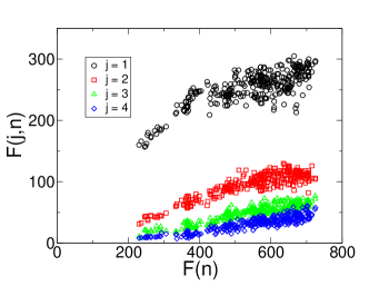
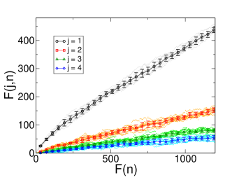
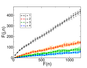
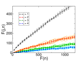
We consider the limit of large $n$, and use the ansatz $F(j,n)=\chi_{j}F(n)$. This ansatz can be justified empirically and by simulations, as shown in Fig. 2, which compares this feature in empirical data and in simulations of different variants of the model.

We have

$$\left\{\begin{array}[]{ccc}\partial_{n}F(n)=&\frac{\alpha\>F(n)\>}{n}\\ \alpha\chi_{1}=&\alpha-\>(1-\alpha)\chi_{1}\\ \alpha\chi_{2}=&(1-\alpha)\chi_{1}-(2-\alpha)\chi_{2}\\ \cdots&\\ \alpha\chi_{j}=&(j-1-\alpha)\chi_{j-1}-(j-\alpha)\chi_{j}\end{array}\right.\ \ ,$$ (12)

giving

$$\left\{\begin{array}[]{ccc}\chi_{1}=&\alpha\\ 2\>\chi_{2}=&(1-\alpha)\>\chi_{1}\\ \cdots&\\ j\>\chi_{j}=&(j-1-\alpha)\>\chi_{j-1}\end{array}\right.\ \ .$$ (13)

The solution of these equations is

$$\chi_{j}=\>\prod_{l=1}^{j-1}(l-\alpha)\frac{1}{\Gamma(j+1)}\>\alpha=\>\frac{\alpha}{\Gamma(1-\alpha)}\cdot(j-1)^{(1-\alpha)}\cdot\frac{\Gamma(j-1)}{\Gamma(j+1)}\ \ ,$$ (14)

which can be estimated as

$$\chi_{j}=\alpha\>\frac{1}{\Gamma(1-\alpha)}\>\left[\frac{1}{j}\right]^{1+\alpha}\ \ ,$$ (15)

giving the result for the scaling of $F(j,n)$ and its prefactor.

IV Direct simulation of the CRP and finite-size effects

Going beyond scaling, the probability distributions generated by a CRP contain large finite-size effects that are relevant for the experimental genome sizes. In this section we analyze the finite size effect affecting the distribution over the domain classes, obtained performing direct numerical simulations of different CRP realizations. The simulations allow to measure $F(n)$, and $F(j,n)$ for finite sizes, and in particular for values of $n$ that are comparable to those of observed genomes shown in Fig. 3.

The normalized distribution of the number of classes with $j$ domains over a genome of length $n$ reaches the theoretical distribution suggested by our model only in the asymptotic limit

$$\frac{F(j,n)}{F(n)}\quad\stackrel{{\scriptstyle n\rightarrow\infty}}{{\longrightarrow}}\quad p_{\alpha}(j)=\frac{\alpha\Gamma(j-\alpha)}{\Gamma(1-\alpha)\Gamma(j+1)}\ .$$ (16)

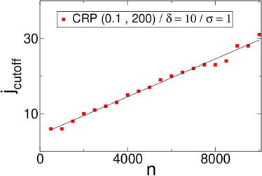
It is possible to obtain more information by studying the ratio of the asymptotic distribution and the distribution obtained from the CRP simulation as shown in Fig. 4. The plot shows that there is a value $m^{*}(n)$, depending on the size $n$ of the genome, beyond which the distribution is not anymore consistent with $p_{\alpha}(j)$ but shows exponential decay and large fluctuations.

In order to obtain a quantitative estimate of the deviation from scaling generating the cutoff, we define an order parameter as follows. Using data obtained from the simulation as in Fig. 4, we find the mean of the first 30 points of the plotted function and then compute the standard deviation $\sigma$ by analyzing windows of $K$ points together. The cutoff is defined when $\sigma>\delta$, where $\delta$ is a parameter. The result of this procedure can be seen in Fig. 4. The cutoff shows a linear dependence from the genome length $n$. To make sure the procedure does not depend too much on the number of iterations $N_{I}$ used to obtain the mean value of $F(j,n)$, we performed it for different values of $N_{I}$. As can be expected (Fig.4), more statistics is needed for probing the cutoff trend in those regions where the probability density function is very small. Were it necessary to obtain from the distribution over domains $n$ an estimate of parameters for the underlying CRP, one could decide to consider only data with $j<j_{\text{cutoff}}$. At the scales that are relevant for empirical data, finite-size corrections are substantial. Indeed, the asymptotic behavior is typically reached for sizes of the order of $n\sim 10^{6}$, where the predictions of the mean-field theory are confirmed. Comparing the histogram of domain occurrence for the mean-field solution of the model, simulations and data, it becomes evident that the intrinsic cutoff set by $n$ causes the observed drift in the fitted exponent of the empirical distribution visible in Fig. 3. This means that the common behavior of the slopes followed by the population of domain classes for genomes of similar sizes can be ascribed to finite-size effects of a common underlying stochastic process.

Figure 3: (Color online) 3 Cumulative distributions for prokaryotes (data from the SUPERFAMILY database). Each is the cumulative histogram of domains in classes for a single genome. 3 Fitted exponent of $F(j,n)$ from empirical data of all prokaryotes, plotted as a function of $n$.

Figure 4: (Color online) 4 Ratio of finite-size and asymptotic value for the distribution of domain classes population $F(j,n)$ taken from 500 realizations of a CRP with $\alpha=0.32$ and $\theta=50$. The three plots corresponds to different value of $n$. 4 Linear $n$-dependency for the cutoff in a CRP. The parameters in the plot are $\alpha=0.1$ and $\theta=200$. A similar trend can be observed for other values of the parameters. 4 Cutoff trends obtained from a CRP with $\alpha=0.44$ and $\theta=60$ and a different number of iterations. The procedure has parameters $K=10$ and $\delta=0.5$.

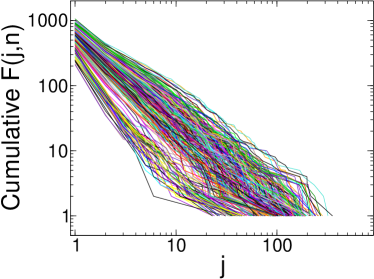
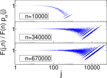
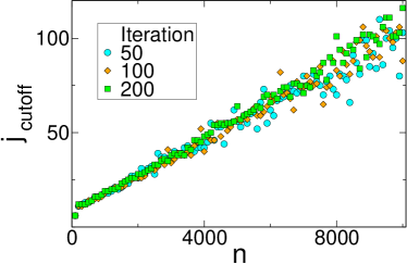
Beyond the linear cutoff, the behavior of the distribution becomes realization-dependent due to the breaking of self-average Bassetti et al. (2009). The relevant parameter to disentangle the realization-dependence is $f$. High-$f$ realizations have different tails of the distribution from low-$f$ ones, giving rise to the large fluctuations observed in Fig. 4. Thus, while the mean-field approach is successful in predicting the asymptotic scaling of the distribution $F(j,n)$, it does not capture the finite-size effects which can be observed in single realization of the CRP process with finite $n$ and $f$. Beyond mean-field is possible to obtain more information by considering the sum of all CRP trajectories conditioned to reaching configurations with given $n$ and $f$.

This enables a statistical-mechanical derivation of the normalized distribution of the number of domains with $f$ classes over a genome of length (number of domains) $n$. Since the focus here is on the mean-field approach, the calculation is described in a parallel work Bassetti et al. (2009).

V Occurrence of domain classes and CRP realizations

The above model does not describe evolutionary time in generations. Conversely, it reproduces random ensembles of different genomes generated one from the other with the basic moves of duplication, innovation (and loss, see below). It considers only events that are observed at a given $n$, independently on when or why they happened in physical or biological time. Genomes from the same realization can be thought of as a trivial tree of life, where each value of $n$ gives a new specie. In the case including domain deletions, more genomes of the same history can have the same size. In contrast, independent realizations are completely unrelated.

The scaling laws in $F(n)$ and $F(j,n)$ hold for the typical realization, indicating that the scaling laws originate from the basic evolutionary moves and not from the fact that the species stem from a common tree with intertwined paths due to common evolutionary history. For example, two completely unrelated realizations will reach similar values of $F$ at the same value of $n$.

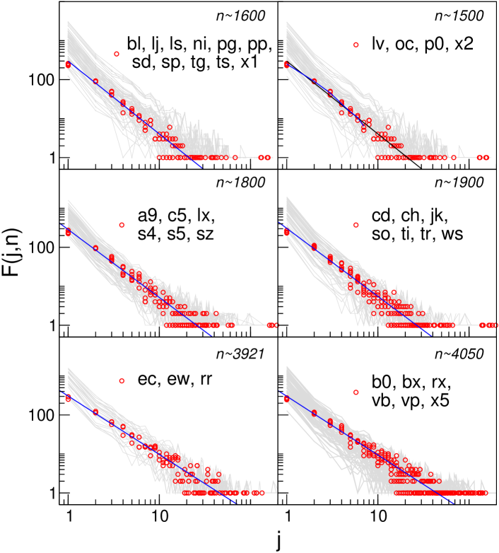
The data confirm this fact: phylogenetically distant bacteria with similar sizes have very similar number and population distribution of domain classes (see Fig. 8).

While the scaling laws are found independently on the realization of the Chinese restaurant model, the uneven occurrence of domain classes can be seen as strongly dependent on common evolutionary history. Averaging over independent realizations, the prediction of the CRP is that the frequency of occurrence of any domain class would be equal, as no class is assigned a specific label. In the Chinese restaurant metaphor, the customers only choose the tables on the basis of their population, and all the tables are equal for any other feature.

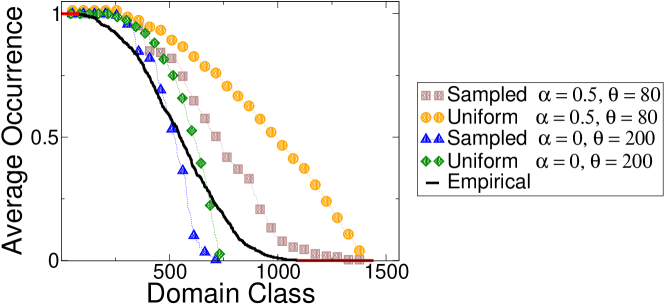
In order to capture this behavior with the model, one can consider the statistics of domain topology occurrence of a single realization, which is an extremely crude, but comparatively more realistic description of common ancestry. In other words, in this case, the classes that appear first are obviously more common among the genomes, and the qualitative phenomenology is restored, without the need of any adjustment in the model definition (Fig. 5).

Figure 5: (Color online) Single realization averages reproduce qualitatively empirical topology occurrence (the fraction of genomes where the given domain topology is found, normalized by the total number of genomes). Domain topology ranked occurrence in typical realizations of the CRP with different parameters (symbols), compared to the empirical data for bacteria (continuous line). The simulated data were obtained considering the occurrence curve for 500 realizations of the process for all sizes from $n=300$ to $n=8000$ (“uniform”), i.e. the range of sizes observed in the data, or directly for the set of empirical sizes of the genomes (“sampled”).

VI Domain Loss

Loss of genes, and thus of domains, is reported to occur frequently in genomes. We will discuss now variants of the model considering the introduction of a domain deletion, or loss rate. The question we ask is whether the introduction of domain loss, which we consider mainly as a perturbation, affects the qualitative behavior of the model, for example by generating different scaling behavior or phase transitions. We will see that the answer to all these questions is mostly negative even for non-infinitesimal perturbations, provided the loss rate is constant and does not scale itself with $F$ and $n$. The main exception to this behavior is found when the loss probability of a domain depends on its own class size.

We introduce domain loss through a new parameter $\delta$, which defines a loss probability $p_{L}$ in two a priori different ways. (1) We can distribute this probability equally among domains, so that the per-class loss probability is $p_{L}^{i}=\delta\frac{k_{i}}{n}$. Consequently, the duplication and innovation probabilities $p_{O}$ and $p_{N}$ are rescaled by a factor $(1-\delta)$. (2) We can also weigh the loss probability of a domain on its own class size, in the same way as domains are duplicated in the standard CRP, so we obtain a per-class loss move with probability $p_{L}^{i}=\delta\frac{k_{i}-\alpha}{n+\theta}$, giving a total $p_{L}=\delta\frac{n-\alpha F}{n+\theta}$ and the rescaling of $p_{O}$ and $p_{N}$. We will see that model (1) and (2) are not equivalent.

On technical grounds, the introduction of domain loss makes the stochastic process entirely different: $n$ is now a random variable, and all the observables that depend on it (e.g. $F(n)$) are stochastic functions of this variable. Another parameter, $t$, describes the iterations of the model. Operatively, we tackle the two models with the usual mean-field approach, writing equations for $n$ and $F$ of the kind $\partial_{t}n=\textsc{q}(n,F)$, $\partial_{t}F=\textsc{r}(n,F)$, and hence obtain the behavior as a function of $n$ by considering $\partial_{n}F=\frac{\textsc{r}(n,F)}{\textsc{q}(n,F)}$. The exact meaning of these equations is not straightforward. For example $F(n)$ should represent the average on all histories passing by $n$, but the differential equation strictly describes only the dependence of the observable from the actual value of the random variable $n$. Nevertheless, the predictions of this mean-field approach agree well with the results of simulations, indicating that these complications typically do not affect the behavior of the means. We will consider situations where, on average, genomes are not shrinking.

Considering model (1), we can write the mean-field equations as

$$\partial_{t}F(t)=(1-\delta)\frac{\alpha F(t)+\theta}{n+\theta}-\delta\frac{F(1,n)}{n}$$ (17)

$$\partial_{t}K_{i}(t)=(1-\delta)\frac{K_{i}(t)-\alpha}{n+\theta}-\delta\frac{K_{i}(t)}{n}\ \ ,$$ (18)

where the sink term for $F$ derives from domain loss in classes with a single element, quantified by $F(1,n)$. Since time does not count genome size, one has to consider the evolution of $n$ with time $t$, given in this case by $\partial_{t}n=1-2\delta$. In order to solve these expressions, we use the ansatz $F(1,n)=\chi_{1}F(n)$, and considering the limit in large $n$. The ansatz is verified by simulations and holds also for empirical data, as previously shown (Fig. 2). The first equation reads:

$$\frac{\partial_{n}{F(n)}}{F(n)}=\frac{1}{n}\left[\frac{(1-\delta)\alpha-\delta\chi_{1}}{1-2\delta}\right]\ \ .$$ (19)

The above equation gives the conventional scaling for $F(n)$ and $K(n)$ with $\alpha$ replaced by $\alpha_{R}=\frac{(1-\delta)\alpha-\delta\chi_{1}}{1-2\delta}$, the correction resulting from the measured value of $\chi_{1}$. By the use of computer simulations we notice that the $\chi_{1}$ coefficient tends to $\alpha$ for infinite-size genomes (Fig. 6, 6, and 6), so that the asymptotic trend of the equally distributed domain loss is identical to that of the standard CRP. This behavior is independent from the chosen $\delta<1/2$, as the asymptotic regime depends only on the growth of $F(n)$, governed by $\alpha$.

Figure 6: (Color online) A model with uniform domain loss (model (1)) does not lead to a change of qualitative behavior with respect to absence of domain loss. We estimated $\chi_{1}$ from simulations with a linear fit of the measured (linear) $F(1,n)$. The measured coefficient $\chi_{1}$ 6 approaches with the parameter $\alpha$, hence the observed scaling exponent $\alpha_{R}$, measured from the simulated $F(n)$ agrees very well with the imposed $\alpha$. 6 This trend is weaker for smaller $\alpha$ but can be regarded as a finite size effect, as the agreement improves 6 for increasing $n$. The plot in (c) refers to $\theta=75,\delta=0.35$. Finally 6, the same phenomenology holds for $\alpha=0$, where the observed parameter $\theta_{R}$ extracted from the behavior of $F(n)$ in simulations agrees well with $\theta$.

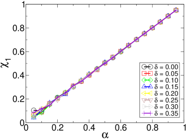
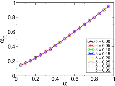
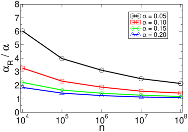
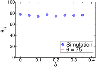
When we analyze the domain distribution of finite-size genomes, we obtain the conventional results: the power-law depends on the genome size, but not on the value of $\delta$ (Fig. 6 and 6). This is explained considering the fact we are comparing runs with fixed genome size, thus with different number of moves, and we do not consider genomes that lose all their own domains. In fact biologically one cannot trace the number of moves needed to reach a specific genome, but essentially we can observe only genomes in their actual state.

More precise results can be obtained by the use of the mean field “master equation” approach sketched above. Using the same ansatz $F(j,n)=\chi_{j}F(n)$, we obtain the following hierarchy of equations for $\chi_{j}$

$$[B+\delta j+(1-\delta)(j-\alpha)]\chi_{j}=(1-\delta)(j-1-\alpha)\chi_{j-1}+\delta(j+1)\chi_{j+1}\ \ ,$$ (20)

with $B=(1-\delta)\alpha-\delta\chi_{1}$ . It is possible to estimate the solution of this system by taking a continuum limit as

$$B\chi(x)+(1-\delta)\partial_{x}[(x-a)\chi(x)]-\delta\partial_{x}\chi(x)=0\ \ ,$$ (21)

which can be solved giving

$$\chi(x)\sim\left[\frac{1}{x}\right]^{1+Z}\ \ ,$$ (22)

with $Z=\frac{B}{1-2\delta}$. We also find $F(n)=n^{Z}$, which is consistent with the constraint $\sum_{j}\>j\chi_{j}=\frac{n}{F(n)}$ since $\sum_{j}\>j\chi_{j}\sim n^{1-Z}$. It is then clear that the introduction of domain loss is equivalent to a rescaling of the parameter $\alpha$ to $\alpha_{R}=Z(\alpha,\delta)$, but in our case, $Z(\alpha,\delta)=\alpha$ asymptotically.

The case $\alpha=0$ has to be treated separately, but the behavior is similar (Fig. 6).

Figure 7: (Color online) In a model with weighted domain loss (model (2)), the loss probability can trigger a transition between two different scaling behaviors for $F(n)$. 7 behavior of observed exponent $\alpha_{R}$ versus $\alpha$ in simulations. The exponent saturates to unity at a critical value that is lower than one. The dashed lines are mean-field predictions in the ansatz of $F(n)$ sublinear in $n$. 7 “Phase-diagram” for the behavior of $\alpha_{R}$ for different values of $\alpha$ and $\delta$. The dashed line is a mean-field estimate of the transition point to $\alpha_{R}=1$, while circles and diamonds are the $\alpha_{R}=.9$ and $\alpha_{R}=.995$ lines from simulations at $n=10^{6}$.

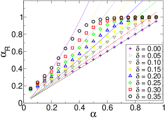
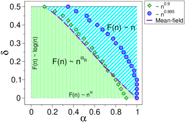
A similar procedure is applicable to model (2). In this case, however, the dependence of the effective death rate from $n$ can bring to an interesting change in the phenomenology, where $\delta$ can select the observed exponent $\alpha_{R}$ and also determine a regime of linear growth for $F(n)$.

To understand this point we can consider the mean-field evolution of $F(n)$. This is determined asymptotically by the balance of a growth term $p_{N}\sim\alpha F/n$ and a loss term $p_{L}\sim\delta F(1,n)(1-\alpha)/n$. With the usual ansatz this gives an asymptotic evolution equation of the kind

$$\partial_{n}F(n)=F(n)\frac{\alpha-\delta(1-\alpha)\chi_{1}}{(1-2\delta)n+2\delta\alpha F(n)}\ ,$$ (23)

with the usual definitions. Simulations confirm the ansatz $F(1,n)=\chi_{1}F(n)$ for this second model, which we will use in the mean-field reasoning. If $F(n)$ is intensive, i.e. asymptotically of order inferior to $n$, the term $2\delta\alpha F$ can be neglected and this equation gives the scaling law $F\sim n^{\alpha_{R}}$, with $\alpha_{R}=\frac{\alpha-\chi_{1}\delta(1-\alpha)}{1-2\delta}$. However, this equation has solution also if $F$ is order $n$, i.e. $\alpha_{R}=1$, and the term $2\delta\alpha F$ in Eq. (23) cannot be neglected. In this case $\alpha$ and $\delta$ determine the prefactor of the scaling law $F\sim n$.

Thus, there are two self-consistent mean-field asymptotic solutions, and we expect a transition between the two distinct behaviors. The existence of this transition is confirmed by simulations (Fig. 7): at fixed $\delta$, $\alpha_{R}$ saturates to $\alpha_{R}\simeq 1$ for larger values of this parameter. The transition point can be understood in mean-field as the intersection of the two solutions $\alpha_{R}=1$ and $\alpha_{R}=\frac{\alpha-\chi_{1}\delta(1-\alpha)}{1-2\delta}$ at varying $\delta$, and gives rise to a two-parameter “phase-diagram” separating the linear from the sublinear scaling of $F(n)$ with $n$, as shown in Fig. 7.

In conclusion, the mean-field approach is effective in exploring the effects of domain loss, which, under some general hypotheses, does not disrupt the basic phenomenology of the duplication-innovation model. Specifically, there appear to be no qualitative changes introduced by a finite uniform loss rate, as long as this rate is constant with $n$. A loss rate that is weighted as the innovation rate, instead, can induce an interesting transition from sublinear to linear scaling.

Thinking about the empirical system, no direct quantitative estimates are currently available regarding the domain loss rate as a function of genome size or number of classes. For this reason, it currently appears difficult to make a definite choice for this ingredient in the model.

VII Models with domain class specificity

In the previous sections we analyzed models that make no distinction between domain topologies, but the latter are selected for duplication moves only on the basis of their population.

It is then clear that they can reproduce the observed qualitative trends for the domain classes and their distributions with one common set of parameters for all genomes. One further question is to estimate the quantitative values of these parameters for the data. While the empirical slope of $F(n)$ could be seen as more compatible with a model having $\alpha=0$, as its slope decays faster than a power law for large values of $n$, the slopes of the power-law distribution of domain classes $P(j,n)$ and their cutoff as a function of $n$ is in closer agreement to a CRP with $\alpha$ between 0.5 and 0.7 Cosentino Lagomarsino et al. (2009).

We will now discuss a CRP variant that is able to distinguish domain classes based on a priori information, thus breaking the symmetry of the model by exchange of tables.

This is equivalent to the introduction of differently colored “tablecloths” labeling the tables, that are determinant in the choice for one table or the other.

Those table colors can be set by any observable of interest. In our analysis, we considered the empirical occurrence of a domain topology as a label. Indeed, the occurrence of a given domain class is determined by its biological function. For example, as expected, all the “core” biological functions such as translation of proteins and DNA replication are performed by highly occurring domain topologies, since this machinery must be present in each genome. Accordingly, these universal classes performing core functions have to appear preferentially earlier on in a model realization. This variant of the model is important for producing informed null models for the analysis of the empirical data, and, as we will see, shows the best agreement with respect to the scaling laws.

Figure 8: (Color online) Comparison of $F(j,n)$ from the SUPERFAMILY Database with mean-field predictions and simulations of the model with class specificity. Comparison between $n-$dependence of powerlaw fit (lines in blue) and universality of the two parameters from our model. Two letters identify each genome, whose full name can be found in Appendix (Table B.1). Simulations (lines in gray) from our model use the same values $\alpha=0.75$ and $\theta=32$.

We will introduce the variant with class specificity by coupling the CRP model to a simple genetic algorithm able to select between innovation moves that choose different classes. Let us first introduce some notation to parametrize domain class occurrence. We define the matrices $\sigma_{i}^{k}$ where:

$$\sigma_{i}^{g}:=\left\{\begin{array}[]{ll}1&\textrm{domain $i$ found in genome $g$}\\ -1&\textrm{domain $i$ not found in genome $g$}\end{array}\right.$$ (24)

It is possible to consider the mean taken along the matrix columns,

$$\left\langle\sigma_{i}^{\textrm{emp}}\right\rangle=\frac{1}{N^{g}}\sum_{g}\sigma_{i}^{g,\textrm{emp}}\ \ ,$$ (25)

where the label “emp” means that this value is obtained from empirical data (Fig. 5).

Generically, a genetic algorithm requires a representation of the space of solution $\Omega$ and a function $f(\omega)$ that tests the quality of the solution computed. In our case, the former is simply the genome obtained from the a CRP step, parametrized by $\sigma_{i}^{k}$. The latter is defined as

$$\mathcal{F}(g)=\prod_{i}\exp\left(\,\sigma_{i}\left\langle\sigma_{i}^{\textrm{emp}}\right\rangle\right)=\exp\left(\,\sum_{i}\sigma_{i}<\sigma_{i}^{\textrm{emp}}>\right)\ \ .$$ (26)

The value of the above scoring function taken over simulated genomes measures how much the set of domain classes they possess agrees with experimental data (in this case on occurrence) and enables to compare different “virtual” CRP moves.

We consider the case of two virtual genomes $g^{{}^{\prime}}$ and $g^{{}^{\prime\prime}}$ generated through standard CRP steps, for simplicity without domain loss, from an initial size $n$ and genome $g(n)$.

Note that in this variant, since the empirical domain topologies are a finite set, domain classes are also finite. As a consequence, tables with a given tablecloth are extracted without replacement, affecting the pool of available colors. As we will see, this is an important requirement to obtain agreement with the data, as it determines the saturation of the function $F(n)$ also for large values of $\alpha$. We will discuss the role of an infinite pool in the following subsection.

Also, as anticipated, domain classes have different “color”, or in mathematical terms the exchangeability of the process is lost. Classes are drawn from the set of the residual ones with uniform probability. Genomes $g^{{}^{\prime}}$ and $g^{{}^{\prime\prime}}$ are compared through the function $\mathcal{F}$ and the highest score one will be the genome $g(n+1)$ so that $g(n+1)=\mathrm{argmax}(\mathcal{F}(g^{{}^{\prime}}),\mathcal{F}(g^{{}^{\prime\prime}}))$.

In these conditions, the rigorous results present in the literature for the CRP cease to be valid. It is still possible, however, to analyze the behavior of this variant by the mean-field approach adopted here, and to compare with simulations. Since the selection rule chooses strictly the maximum, it is essentially able to distinguish the sign of $\langle\sigma^{\textrm{emp}}_{i}\rangle$ only. For this reason, it is sufficient to account for the positivity (which we label by “+”) and negativity (“-”) of this function for a given domain index $i$. This means that, with the simplification of two virtual moves only, the model introduces only one extra effective parameter, i.e. the ratio of the “universal” (positive $\mathcal{F}$) to the “contextual” (negative $\mathcal{F}$) domain classes.

In order to write the mean-field equations for this model variant, we first have to classify all the possible outcomes of the virtual CRP moves. The genomes $g^{{}^{\prime}}$ and $g^{{}^{\prime\prime}}$ proposed by the CRP proliferation step can have the same (labeled by “$1$”), higher (“$1_{+}$”) or lower (“$1_{-}$”) score than their parent, depending on $p_{O}$, $p_{N}$ and by the probabilities to draw a universal or contextual domain family, $p_{+}$ and $p_{-}$ respectively. Using these labels, the scheme of the possible states and their outcome in the selection step is given in Table 1.

proliferation $(g^{{}^{\prime}},g^{{}^{\prime\prime}})$	probability	selection
$(1,1)$	$p_{O}^{2}$	old
$(1,1_{-})$	$2\>p_{O}\>p_{N}\>p_{-}$	old
$(1,1_{+})$	$2\>p_{O}\>p_{N}\>p_{+}$	new+
$(1_{+},1_{+})$	$p_{N}^{2}\>p_{+}^{2}$	new+
$(1_{+},1_{-})$	$2\>p_{N}^{2}\>p_{-}\>p_{+}$	new+
$(1_{-},1_{-})$	$p_{N}^{2}\>p_{-}^{2}$	new-

Table 1: Compound probabilities of picking up a new domain or an old domain with positive or negative cost function.

From the Table 1, it is straightforward to derive the modified duplication and innovation probabilities $\hat{p}_{O}$ and $\hat{p}_{N}$ of the complete algorithmic iteration:

$$\hat{p}_{O}=p_{O}\>(p_{O}+2\>p_{N}p_{-})$$ (27)

$$\hat{p}_{N}=p_{N}\>(p_{N}+2\>p_{O}p_{+})=p_{N+}+p_{N-}\ \ ,$$ (28)

where $p_{N+}=p_{N}p_{+}(2-p_{N}p_{+})$ and $p_{N-}=p_{N}^{2}(1-p_{+})^{2}$ are the probabilities that the new domain is drawn from the universal or contextual families respectively.

We now write the macroscopic evolution equation for the number of domain families by the usual procedure. Calling $K^{+}(n)$ and $K^{-}(n)$ the number of domain classes that have positive or negative $\langle\sigma^{\textrm{emp}}_{i}\rangle$ and are not represented in $g(n)$,

$$\left\{\begin{array}[]{cc}\partial_{n}F(n)=&\hat{p}_{N}\\ \partial_{n}K^{+}(n)=&-\hat{p}_{N+}\\ \partial_{n}K^{-}(n)=&-\hat{p}_{N-}\\ \end{array}\right.\ \ .$$ (29)

Now, $p_{+}=K^{+}/(K^{-}+K^{+})=K^{+}/(D-F(n))$, so that we can rewrite

$$\left\{\begin{array}[]{cc}\partial_{n}F(n)=&(\frac{\alpha F(n)+\theta}{n+\theta})\>\Big{[}\frac{\alpha F(n)+\theta}{n+\theta}\>+\>\frac{2K^{+}(n)}{D-F(n)}(\frac{n-\alpha F(n)}{n+\theta})\Big{]}\\ \partial_{n}K^{+}(n)=&-(\frac{\alpha F(n)+\theta}{n+\theta})\>\frac{K^{+}(t)}{D-F(n)}\>\Big{[}2-\>(\frac{\alpha F(n)+\theta}{n+\theta})\frac{K^{+}(n)}{D-F(n)}\Big{]}\\ \partial_{n}K^{-}(n)=&-(\frac{\alpha F(n)+\theta}{n+\theta})^{2}\>(\frac{K^{+}(n)}{D-F(n)})^{2}\end{array}\right.\ \ .$$ (30)

The above equations have the following consistency properties

• $\partial_{n}\Big{(}K^{+}+K^{-}+F\Big{)}=0$, hence $K^{+}+K^{-}+F=D\quad\forall n$.

• $\partial_{n}F\leq 1$, hence $F(n)\leq n$.

• $\partial_{n}F\geq 0$, $\partial_{n}K^{+}\geq 0$ and $\partial_{n}(F+K^{+})\geq 0$ so that $F$ grows faster than $K^{+}$ decreases.

Choosing the initial conditions from empirical data $n_{0},F(n_{0})$, size and number of domain classes of the smallest genome, we have, since $F(n_{0})<n_{0}$ and $\alpha\leq 1$,

$$\frac{\alpha F(n_{0})+\theta}{n_{0}+\theta}<1\ \ .$$ (31)

It is simple to verify that under this condition the system always has solutions that relax to a finite value $F_{\infty}<D$. Indeed, after the time $n^{*}$ where $K^{+}(n*)=0$, the equations reduce to $\partial_{n}K^{+}=0$, $K^{-}=D-F$ and

$$\partial_{n}F(n)=\left(\frac{\alpha F(n)+\theta}{n+\theta}\right)^{2}\ \ ,$$ (32)

immediately giving our result. It is important to notice that this result depends on the fact the empirical reservoir of domains is finite (and thus on the biological hypothesis that the full pool of available domain topologies is). Indeed, in presence of an infinite reservoir of domain classes, $F(n)$ does not relax to a finite value. In this case, similarly as in the case of non uniform loss, there is a transition from linear to sublinear scaling piloted by the parameters $p_{+}$ and $\alpha$. If $2p_{+}\alpha<1$, $F\sim n^{2p_{+}\alpha}$, while if $2p_{+}\alpha>1$, $F\sim n$.

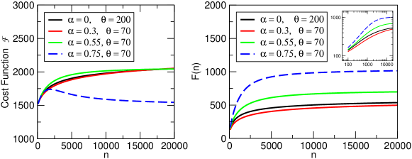
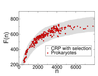
Numerical solutions of Eq. (30) give the same behavior for $F(n)$ as the direct simulations (Fig. 9). In particular, while this function grows as a power law for small genome sizes, it saturates at the relevant scale, giving good agreement with the data (Fig. 10). The internal laws of domain usage of this model were obtained from direct simulations only, and give a good quantitative agreement with the data (Fig. 10). Finally, Fig. 9 also shows that, for large values of $\alpha$ (above $0.7$) this function reaches a maximum at sizes between 2000 and 4000. This is also where most of the empirical genomes are found, indicating that this range of genome sizes may allow the optimal usage of universal and contextual domain families.

Figure 9: (Color online) Numerical solutions of the mean-field equations of the CRP model with selection of specific domain classes. Left panel: score function $\mathcal{F}(n)$ for different values of $\alpha$. Right panel: $F(n)$ plotted in linear and logarithmic (inset) scales.

Figure 10: (Color online) Comparison of the CRP with class specificity with experimental data. CRP parameters are $\alpha=0.75$ e $\theta=0.32$. Number of domain classes versus the length $n$ of genome. Simulations were performed for $n<10000$ taking data at each interval of $1000$ units in size, and considering 5 realizations at each step.

VIII Conclusions

We presented from a statistical physics viewpoint a class of duplication-innovation-loss stochastic processes able to describe the probability distributions and scaling laws observed in genomic data sets for protein structural domains with few effective parameters. These models are different declinations of the basic paradigm set by the Chinese restaurant process which, though much explored in the statistical literature, remains relatively unexplored by the physics community, despite of its rich and peculiar phenomenology, which could make it useful in multiple applications.

Our focus has been to present the basic phenomenology of different variants of the model connected to possibly relevant aspects of the evolutionary dynamics of protein domains, prominently domain duplication, innovation, loss, and the specificity of domain classes. In doing this, we have shown how a mean-field approach, despite of its simplicity, can be extremely powerful in the analysis of the qualitative behavior of this class of models. More subtle aspects of these models might be approached by simulations and refined statistical mechanics methods, directly accessing the sum on all different paths.

For the standard CRP, we have shown how the scaling laws in the number and in the slope of the observed power-law distributions of domain classes are qualitatively reproduced, by the typical or the average realization. The salient ingredient for this feature is that this model can include the correct relative scaling of innovation to duplication moves, which can be generated by statistical dependence of innovation, or by the fact that the process of domain birth does not give rise to identically distributed random variables at different sizes.

The mean-field results can be obtained in two independent ways: with dynamic equations for the population and number of domain classes, or, similarly as for the Zero-range process Evans and Hanney (2005), by considering the evolution of the number of classes with a given population. The latter “master equation” approach gives access to the full histogram of domain class population. The scaling of the slope of the domain class distributions can be understood as a finite-size effect on these histograms. We have also shown how the uneven occurrence of domain classes can be explained by the CRP provided one considers the statistics of occurrence in a single realization. This can be interpreted as the fact that genomes are related by common evolutionary paths.

This phenomenology is extremely robust to the introduction of finite domain loss probabilities that do not scale with $n$ or $F$. For uniform domain loss, the full mean-field equations are still accessible analytically, and point to the effect of domain loss as a simple effective rescaling of the model parameters. The presence of a loss rate that scales with size, instead, can trigger a transition from sublinear to linear scaling in the number of distinct classes.

Finally, we have discussed the case of models that introduce the specificity of domain classes, and thus explicitly breaks the symmetry between them, as expected for the biological case. Such variants can be very useful in more detailed statistical investigations (e.g. as a null model) and to define inference problems on the available bioinformatic data.

For example, a preferential duplication of conserved proteins has been reported in eukaryotes Davis and Petrov (2004), and could be tested against a duplication-innovation-loss model where a “conservation index” characterizes specificity.

Here, we have shown how a CRP variant with specificity can be formulated as a genetic algorithm where different CRP virtual moves are selected on the basis of an informed scoring function, defined on the basis of further empirical observables related to domain classes (such as function, correlated occurrence, etc.) In our case, we have shown how such a variant, weighting the virtual moves according to the observed occurrence of the finite pool of domain classes has very good quantitative agreement with the available data.

The future perspective on this systems and models are abundant, both for the application of the models to the genomics of protein domains, where the most promising ways seems to be the use in specific inference problems on species with known evolutionary histories, and in other problems of statistical physics and complex systems, for example to develop new growth models for complex networks where the nodes can evolve with similar moves. One prominent example is the case of protein-protein interaction networks, graphs where the nodes follow a dynamics that is coupled to those of protein domains, while the edges can be inherited by duplication, lost, or rewired by mutation and natural selection.

Appendix A Data and methods

All the data considered here were extracted from the SUPERFAMILY database version 1.69 and 1.73. We considered domains at the superfamily level, although similar results hold for folds and families. A genome “size” $n$ was defined as the number of domain hits for each genome. The main data structures considered were the number of domain classes and the histograms of domain class population. We also considered the ranked occurrence of a given domain class across genomes.

The different variants of the duplication-innovation-loss model were simulated directly using a C++ code and compared with the mean-field results and the empirical data. The variant with class specificity couples the CRP model to a simple genetic algorithm selecting innovation moves that choose distinct classes, on the basis of their empirical occurrence. For all the variants, we derived and solved the mean-field equations for the evolution of the main observables, and described alternative approaches for their solution.

The finite-size behavior of a CRP was studied comparing the finite-size histograms obtained from direct simulations with the asymptotic limit of the exact analytical result (formula 16) Pitman (2002), and defining a cutoff as the class-size where the deviation was larger than an arbitrary threshold. The cutoff was studied as a function of $n$. For the CRP variants with specificity and domain loss only the mean-field solution given here is available for the same analysis. The exponent of the empirical domain class distributions for genomes with different size was estimated from a power-law fit of the cumulative histograms, keeping into account the finite-size cutoff.

Appendix B List of Bacteria Used in the Analysis of Fig. 8

Abbreviation	Full Name
a9	Streptococcus agalactiae A9
b0	Bacillus anthracis Sterne
b1	Baumannia cicadellinicola Hc
bl	Bifidobacterium longum NCC2705
bx	Bacillus cereus ATCC 10987
c5	Chlorobium chlorochromatii CaD
cd	Corynebacterium diphtheriae NCTC 13129
ch	Chlorobium tepidum TLS
ec	Escherichia coli K12
ew	Escherichia coli W3110
jk	Corynebacterium jeikeium K411
lj	Lactobacillus johnsonii NCC 533
ls	Lactobacillus sakei ssp. sakei 23K
lv	Lactobacillus salivarius ssp. salivarius UCC118
lx	Leifsonia xyli ssp. xyli CTCB07
ni	Neisseria gonorrhoeae FA 1090
oc	Prochlorococcus marinus NATL2A
p0	Candidatus Protochlamydia amoebophila UWE25
pg	Porphyromonas gingivalis W83
pp	Streptococcus pyogenes MGAS2096
rr	Rhodopseudomonas palustris BisB5
rx	Rhodoferax ferrireducens T118
s4	Streptococcus agalactiae 2603V/R
s5	Streptococcus agalactiae NEM316
sd	Streptococcus thermophilus LMG 18311
so	Synechococcus sp. CC9605
sp	Streptococcus pyogenes MGAS10394
sz	Synechococcus sp. CC9902
tg	Streptococcus pyogenes MGAS10750
ti	Thiomicrospira denitrificans ATCC 33889
tr	Thermus thermophilus HB8
ts	Streptococcus pyogenes MGAS10270
vb	Vibrio vulnificus YJ016
vp	Vibrio parahaemolyticus RIMD 2210633
ws	Wolinella succinogenes DSM 1740
x1	Streptococcus thermophilus CNRZ1066
x2	Streptococcus pyogenes M1 GAS
x5	Bacillus cereus E33L

Table B.1: Abbreviations used for the genomes in Fig. 8.