Driven Disordered Polymorphic Solids: Phases and Phase Transitions, Dynamical Coexistence and Peak Effect Anomalies

Abstract

We study a simple model for the depinning and driven steady state phases of a solid tuned across a polymorphic phase transition between ground states of triangular and square symmetry. The competition between the underlying structural phase transition in the pure system and the effects of the underlying disorder, as modified by the drive, stabilizes a variety of unusual dynamical phases. These include pinned states which may have dominantly triangular or square correlations, a plastically flowing liquid-like phase, a moving phase with hexatic correlations, flowing triangular and square states and a dynamic coexistence regime characterized by the complex interconversion of locally square and triangular regions. We locate these phases in a dynamical phase diagram and study them by defining and measuring appropriate order-parameters and their correlations. We demonstrate that the apparent power-law orientational correlations we obtain in our moving hexatic phase arise from circularly averaging an orientational correlation function which exhibits long-range order in the (longitudinal) drive direction and short-range order in the transverse direction. This calls previous simulation-based assignments of the driven hexatic glass into question. The intermediate coexistence regime exhibits several novel properties, including substantial enhancement in the current noise, an unusual power-law spectrum of current fluctuations and striking metastability effects. We show that this noise arises from the fluctuations of the interface separating locally square and triangular ordered regions by demonstrating a correlation between enhanced velocity fluctuations and local coordinations intermediate between the square and triangular. We demonstrate the breakdown of effective “shaking temperature” treatments in the coexistence regime by showing that such shaking temperatures are non-monotonic functions of the drive in this regime. Finally we discuss the relevance of these simulations to the anomalous behaviour seen in the peak effect regime of vortex lines in the disordered mixed phase of type-II superconductors. We propose that this anomalous behavior is directly linked to the behavior exhibited in our simulations in the dynamical coexistence regime, thus suggesting a possible solution to the problem of the origin of peak effect anomalies.

I Introduction

The motion of an elastic medium across a quenched disordered background presents a simple paradigm for the understanding of several experimentsFisher (1998). These include studies of the depinning of charge-density wavesGrüner (1988); Thorne (2005), transport measurements in the mixed phase of type-II superconductorsGiamarchi and Bhattacharya (2002) as well as measurements of the flow of colloidal particles across rough substratesPertsinidis and Ling (2008); Reichhardt and Olson (2002). The issue of universality at continuous depinning transitions has traditionally dominated much of this literature, especially in the CDW contextFisher (1985). However, the behaviour of non-universal quantities in the vicinity of the depinning transition is often of more interest to the experimenterHiggins and Bhattacharya (1996). The nature of order, correlations and response within the moving phase are also questions which underly many recent investigations of the physics of non-equilibrium steady states, motivated in large part by the considerable experimental literature on dynamical states of flux lines in the mixed phase of driven, disordered type-II superconductorsHiggins and Bhattacharya (1996).

The canonical example of a remarkable non-universal feature of the depinning transition is the peak effect often seen in the mixed phase in the vicinity of the upper critical field $H_{c2}$Berlincourt et al. (1961). The peak effect, a generic property of weakly disordered type-II superconductors, describes the non-monotonic behaviour of the critical current $j_{c}$ as a function of the temperature $T$ or applied magnetic field $H$Campbell and Evetts (1972). This critical current measures the (depinning) force required to induce observable motion of the vortex line arrayCampbell and Evetts (1972); Tinkham (1975). The peak effect is an often spectacular phenomenon, with $j_{c}$ rising sharply in a narrow region whose width is comparable to that of the zero-field superconducting transitionHiggins and Bhattacharya (1996). Investigations of the peak effect describe a host of unusual phenomena associated with this narrow regimeHiggins and Bhattacharya (1996). These include “finger print phenomena”, slow voltage oscillations, history dependent dynamic response, enhanced low-frequency noise with a $1/f^{\alpha}$ spectrum and many other remarkable features. These are often collectively referred to as “peak effect anomalies” Bhattacharya and Higgins (1993, 1994, 1995); Marley et al. (1995); Merithew et al. (1996); Henderson et al. (1996); Ghosh et al. (1996); Ravikumar et al. (1998); Banerjee et al. (1998, 1999, 2001); Henderson et al. (1998); Xiao et al. (1999).

Approaches to understanding the peak effect have typically followed two distinct paths. The first views the peak effect as arising solely from the softening of the flux-lattice close to H_c2, as reflected in the vanishing of the shear elastic constant $C_{66}\sim(H-H_{c2})^{2}$, while pinning strengths soften more gradually, as $(H-H_{c2})$Pippard (1969). As suggested initially by PippardPippard (1969), softer lattices should be able to adapt better to random pinningLarkin and Ovchinnikov (1974, 1979). In the second class of theories, the peak effect is a reflection of the underlying phase diagram of a weakly pinned, flux-line array in the $H-T$ planeGiamarchi and Le Doussal (1995, 1997); van Otterlo et al. (1998); Nonomura and Hu (2001); Olsson and Teitel (2009); Vinokur et al. (1998); Dasgupta and Valls (2007); Menon (2001, 2002a, 2002b); Divakar et al. (2004); Menon et al. (2006); Olson et al. (2001a, b); Mikitik and Brandt (2001); Rosenstein and Li (2009). It has been argued that such phase diagrams should generically accomodate intermediate glassy phases close to the melting transitionVinokur et al. (1998); Giamarchi and Le Doussal (1997); Banerjee et al. (2001); Menon (2001, 2002a, 2002b). The peak effect is then proposed to be associated with abrupt changes in transport across such phase boundaries, with the anomalies rationalized in terms of the glassy nature of such intermediate statesBanerjee et al. (2001); Menon (2001, 2002a, 2002b); Mikitik and Brandt (2001).

A third, as yet unexplored, alternative to these approaches which addresses the origin of the anomalies directly, combines the scenario of an underlying static phase transition with the possibility that driving such a system induces dynamical steady states with no static counterpart. With this motivation in mind, the central questions addressed in this paper are the following: Consider an underlying static phase transition in a pure system as modified or broadened by weak quenched disorder. How are signals of this transition manifest in dynamical measurements? Further, can novel dynamical states with no analog in either the pure or the disordered undriven system be obtained once the system is driven? Finally, could some of the remarkable phenomenology of the peak effect anomalies possibly originate in the properties of such states?

We recently proposed a suitable model system capable of addressing some of these issuesSengupta et al. (2007, 2007). Our model uses interacting particles in two dimensions close to zero temperature. These particles form a crystal in the absence of disorder. The interaction potential contains a simple two-body repulsive power-law interaction as well as a short-range three-body interaction. The two-body interaction favours a triangular lattice. The three-body term favours a square lattice. We tune between a square and a triangular ground state by varying the strength of a single parameter, the coefficient of the three-body interaction $v_{3}$. We place $N$ such interacting particles in a quenched disordered background, modeled numerically in terms of a Gaussian random field with specified strength and two-point correlations. After finding the ground state of the interacting particles in the disordered background using simulated annealing techniques, we apply a uniform driving force to the particles. This results, first, in a depinning transition and then a sequence of partially ordered states with varying degrees of spatial correlations as the force is increased.

The advantages to such a formulation are several. Signatures of phase transitions in dynamical measurements are typically overwhelmed by thermal fluctuations for purely temperature driven transitions, thereby obscuring the very effects we wish to characterize. Our model of a $T=0$ transition between square and triangular phases surmounts this problem while also mirroring similar structural phase transitions in vortex lattices, typically between triangular and distorted rectangular phases, across which broadened peak effects are seen Dewhurst et al. (2005); Vinnikov et al. (2001); Rosenstein et al. (2005); White et al. (2008); Mesot et al. (2005).

The sequence of steady states obtained in our model as a function of the uniform external driving force $F$ acting on the particles, and for various values of the three-body interaction strength $v_{3}$, is summarized in the dynamical “phase” diagram of Fig. 1. This phase diagram extends a similar phase diagram proposed earlier to much larger values of $v_{3}$Sengupta et al. (2007, 2007). The phase diagram shows a variety of phases: pinned states which may have dominantly triangular or square correlations, a plastically flowing “liquid-like” state, a moving anisotropic hexatic phase, flowing triangular and square states ordered over the size of our simulation cell and a dynamic coexistence regime.

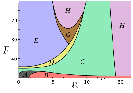
Figure 1: [Color Online]: Schematic Dynamical Phase Diagram of our model system, plotted as a function of the three-body interaction strength $v_{3}$ and of driving force $F$ (see text for a more detailed discussion). The phases are (A) pinned triangular (B) pinned square (C) plastic flow (D) anisotropic hexatic (E) flowing triangular (G) coexistence regime and (H) flowing square. The precise location of the lines separating these phases is disorder-dependent, although the general topology of the phase diagram is not sensitive to disorder. The boundary separating plastic flow from the flowing square phase is a very strong function of the driving force $F$ at large $v_{3}$.

This paper presents a detailed characterization of these states. We define and calculate appropriate correlation functions for $n-$atic (where $n=6$, mostly) orientational order, in addition to structure factors measuring the distribution of particles. We capture local bond-orientational order in terms of distribution functions of a complex number characterizing the local orientation. This representation is used to understand the action of an external force in biasing the axes of orientational order. We demonstrate that the hexatic order we measure arises as an artefact of averaging an anisotropic quantity, which decays either exponentially to zero or to a constant value along two principal directions. In the “ordered” moving phases, square and triangular, shown in Fig. 1, orientational order appears to be established over length scales much large than our system sizes.

In the coexistence regime (labeled (G) in the phase diagram of Fig. 1), we investigate the nucleation and growth of ordered domains of one type (square or triangular) in another. Such nuclei are, in general, anisotropic, forming along the principal crystalline directions of each phase. The interface region of different domains is remarkably dynamic. We assign the substantial increase in noise we see within the coexistence regime to the unusual properties of this interface, quantifying this proposal by linking measures of fluctuation magnitude to coordinations intermediate between square and triangular.

We measure several quantities on the dynamical side, including the basic current-force relations, current statistics and current noise at many different points in the phase diagram. We calculate the Koshelev-Vinokur “shaking temperature”Koshelev and Vinokur (1994), defined in detail below, to understand how disorder-induced fluctuations in the flow might provide an effective, pure-system temperature in terms of which phase behaviour can be discussed. This shaking temperature, while a monotonically decreasing function of the applied force over much of the $F-v_{3}$ phase diagram, is strikingly non-monotonic in $F$ within the coexistence regime. We correlate local orientational and density fluctuations within the coexistence state to understand the origins of the anomalous noise in the coexistence regime. We compare the phenomenology of the simulations, specifically relating to the coexistence regime, to what is seen in experiments on peak effect anomalies in the mixed state. We argue that this comparison, supported by general phenomenological arguments, suggests strongly that there may be a generic explanation for peak effect anomalies.

The outline of this paper is the following. In Section II, we describe the model system we use, explaining our methodology and discussing relevant features of the simulations and what we calculate. In Section III, we provide an overview of the phase diagram of the driven system, discussing, in particular detail, the hexatic vortex glass and the coexistence phase. We discuss growth and fluctuations of one phase within another, the behaviour upon quenching and the origins of noise in this regime. In Section IV, we discuss some aspects of peak effect anomalies seen in the experiments, pointing out the close relationship between the diversity we see in our simulations with the experimental data. We then conjecture that behaviour analogous to what we see in the coexistence regime may be generic to all driven disordered systems in the vicinity of an underlying static first-order phase transition in the pure limit. Finally, in our concluding section, Section V, we summarize our results briefly and suggest further lines of research.

II The Model System and Methodology

Our model system is two-dimensional and consists of particles with two and three-body interactionsSengupta et al. (2007, 2007). The three-body interaction, parametrized through a single parameter $v_{3}$, tunes the system across a square-triangular phase transition. The total interaction energy for particles confined to two-dimensions and labelled by their position vectors ${\bf r}_{i}$ is thus

$$V=1/2\sum_{i\neq j}V_{2}(r_{ij})+1/6\sum_{i\neq j\neq k}V_{3}(r_{i},r_{j},r_{k}),$$ (1)

where $r_{ij}\equiv|{\bf r}_{ij}|\equiv|{\bf r}_{j}-{\bf r}_{i}|$.

We take the two-body interaction to be of the power-law form

$$V_{2}(r_{ij})=v_{2}(\frac{\sigma_{0}}{r_{ij}})^{12},$$ (2)

while the three-body term is

$$V_{3}(r_{i},r_{j},r_{k})=v_{3}[f_{ij}sin^{2}(4\theta_{ijk})f_{jk}+{\rm permutations}].$$ (3)

The function $f_{ij}\equiv f(r_{ij})=(r_{ij}-r_{0})^{2}$ for $r_{ij}<1.8\sigma_{0}$ and $0$ otherwise and $\theta_{ijk}$ is the angle between ${\bf r}_{ji}$ and ${\bf r}_{jk}$.

The two-body interaction favors a triangular ground state while the three-body term favors $90^{\circ}$ and $45^{\circ}$ bonds and hence a square structure. Energy and length scales are set using $v_{2}=1$ and $\sigma_{0}=1$. The zero-temperature phase diagram for particles interacting with this potential has been calculated in Ref. Bhattacharya et al. (2008). As a function of the parameter $v_{3}$, which measures the strength of the three-body term, a discontinuous transition between a triangular lattice, obtained for $v_{3}<1.5$, and a square lattice, obtained for $v_{3}>1.5$, is seen. A similar potential was used by Stillinger and Weber in an early study of melting of a square solidWeber and Stillinger (1993).

Particles also interact with background quenched disorder in the form of a one-body Gaussian random potential field V${}_{d}({\bf r})$ with zero mean and exponentially decaying (short-range) correlations. This potential field is defined on a fine grid following a methodology due to Chudnovsky and DickmanChudnovsky and Dickman (1998), and interpolation is used to find the value of the potential at intermediate pointsSengupta et al. (2005). The disorder variance is set to $v_{d}^{2}=1$ and its spatial correlation length is $\xi=0.12$. Larkin length estimatesLarkin and Ovchinnikov (1974, 1979); Giamarchi and Bhattacharya (2002) yield $L_{a}/a\sim 100$, with $a=1/{\rho}^{1/2}$ the lattice parameter, somewhat larger than our system size.

II.1 Methodology

The system evolves through standard Langevin dynamics;

$$\dot{{\bf r}_{i}} = {\bf v}_{i},$$

$$\dot{{\bf v}_{i}} = {{\bf f}_{i}}^{\rm int}-\gamma{\bf v}_{i}+{\bf F}+{\bf\eta}_{i}(t).$$ (4)

Here ${\bf v}_{i}$ is the velocity, ${{\bf f}_{i}}^{\rm int}$ the total interaction force, and ${\bf\eta}_{i}(t)$ the random force acting on particle $i$, simulating thermal fluctuations at temperature $T$. A constant force ${\bf F}=\{F_{x},0\}$ drives the system. The zero-mean thermal noise ${\bf\eta}_{i}(t)$ is specified by

$$<{\bf\eta}_{i}(t){\bf}{\bf\eta}_{j}(t^{\prime})>=2T\gamma\delta_{ij}\delta(t-t^{\prime}),$$ (5)

with $T=0.1$, well below the equilibrium melting temperature of the system. The unit of time $\tau=\gamma\sigma_{0}^{2}/v_{2}$, with $\gamma=1$ the viscosity.

II.2 Simulation details

Our system consists of $N$ particles, with $N$ between $1600$ and $10,000$, in a square box at number density $\rho=1.1$. Configurations obtained through a simulated annealing procedure are the initial inputs to our Langevin simulations. This annealing procedure involves equilibration using a NVT Monte Carlo scheme at fixed density and within a fixed background potential of a tunable amplitude. The strength of the disorder is then increased in steps to the working disorder strength, with the system equilibrated at each step for around $10^{5}$ Monte Carlo steps. Varying the strength of disorder in this fashion enables the system to converge to its true minimum energy state more efficiently than methods which employ a temperature annealing schedule.

We evolve the system using a time step of $10^{-4}\tau$. The external force $F_{x}$ is ramped up from a starting value of 0, with the system maintained at upto $10^{8}$ steps at each $F_{x}$.

Given the local instantaneous particle density

$$\rho({\bf r},t)=\sum_{i}\delta({\bf r}-r_{i}(t)),$$ (6)

we calculate a variety of structural observables at equal time, such as the static structure factor $S({\bf q})$ defined by

$$S({\bf q})=\sum_{ij}\exp(-i{\bf q\cdot r}_{ij}).$$ (7)

where ${\bf r}_{ij}={\bf r}_{i}-{\bf r}_{j}$. Delaunay triangulations yield the probability distributions $P(n)$ of $n=4,5,6$ and $7$ coordinated particles ($\sum_{n}P(n)=1$)Preparata and Shamos (1985). We define order parameters

$$\psi=(P(4)-P(6))/(P(4)+P(6)),$$ (8)

to distinguish between square and triangular phases,

$$\psi_{\Delta}=(P(6)-P(5)-P(7))/(P(6)+P(5)+P(7)),$$ (9)

to distinguish between liquid (disordered) and triangular crystals and

$$\psi_{\Box}=(P(4)-P(5)-P(7))/(P(4)+P(5)+P(7)),$$ (10)

to distinguish between liquid and square crystals. In addition, we compute the hexatic order parameter

$$\psi_{6,i}\equiv\psi_{6}({\bf r}_{i})=\sum_{j}\exp(-i6\theta_{ij}),$$ (11)

and its correlations, defined via

$$g_{6}(r)=\langle\psi_{6}(0)\psi_{6}(r)\rangle$$ (12)

where $\theta$ defines the bond angle associated with the vector connecting neighbouring particles, as measured with respect to an arbitrary external axis. The second moment of the distribution of $\psi_{6,i}$ is the bond-orientational susceptibility. Below, we describe alternative distribution functions which quantify the extent to which the axes of the crystal align along the driving force direction. These include “Argand plots” of the distribution of a complex quantity which characterizes local orientational order.

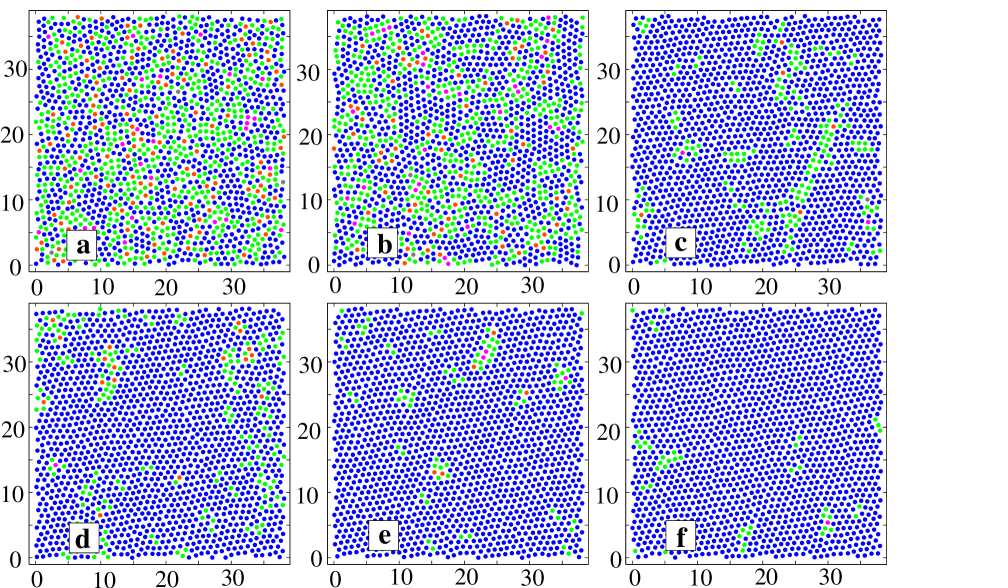
Figure 2: [Color Online]: Instantaneous snapshots of steady state configurations of the system at $T=0.1$ with $v_{3}=6.0$. The configurations (a) - (f) are respectively for driving forces $F_{x}=6,10,20,22,32$ and $40$ respectively. The particles are colored according to their coordination number $n$ = 4 (magenta), 5 (green), 6 (blue), 7 (orange) and 8 (grey), as obtained from Delaunay triangulations.

The dynamical variables we study include the center of mass velocity $v_{cm}$, and the particle flux and its statistics. The centre-of-mass velocity is defined via

$$v_{cm}=\langle\frac{1}{N}\sum_{i}v_{i}(t)\rangle,$$ (13)

where the brackets $\langle\cdot\rangle$ denote an average in steady state and $v_{i}(t)$ is the velocity of particle $i$ at time $t$. We measure the particle flux by counting the number of particles which cross an imaginary line crossing the $x=0$ axis in a single time step and then averaging this result over time. This flux, essentially a current $j(x,y)$ integrated over all $y$ at fixed x, which must be independent of $x$ in steady state, has fluctuations about a constant value. We measure and discuss the power spectrum of these fluctuations.

Koshelev and Vinokur (KV)Koshelev and Vinokur (1994) have suggested that the combination of the drive and the disorder should yield an effective “shaking” temperature in the moving phase. Such an effective temperature manifests itself in transverse and longitudinal fluctuations of the velocity. We calculate the KV shaking temperature $T^{\nu}_{sh}$Koshelev and Vinokur (1994) appropriate to the drive and transverse directions, obtaining it from

$$T^{\nu}_{sh}=\langle\sum_{i}^{N}(v_{i}^{\nu}-v^{\nu}_{cm})^{2}\rangle/2N,~{}~{}~{}~{}~{}~{}\nu=x,y.$$ (14)

We measure the variation of the $T^{\nu}$’s as a function both of force and $v_{3}$ at various points in our phase diagram.

The transition to the coexistence phase is marked by the growth of highly anisotropic, obliquely inclined square nuclei, in a background of approximately triangularly coordinated solid. To understand their role in the nucleation kinetics, we define and compute quantities which measure the anisotropy of such clusters. To determine the source of excess noise in the coexistence phase, we measure the probability distribution of the instantaneous velocity excess above the mean, as a function of the local coordination as well as of the local density. As we show below, these measurements indicate that the substantial portion of the noise originates from regions which are neither wholly square or triangular but to be found at the interface between such locally ordered states.

III Phases and Phase Diagram of the Driven System

A qualitative understanding of the basic structure of the phase diagram of Fig. 1 can be obtained from snapshots of instantaneous configurations in the steady state. Such snapshots are shown in Fig. 2, obtained from simulations at $T=0.1$ with $v_{3}=6.0$. The configurations labelled (a)-(f) are for driving forces $F_{x}(=F)=6,10,20,22,32$ and $40$ respectively. Particles are colored according to their coordination number $n$ = 4 (magenta), 5 (green), 6 (blue), 7 (orange) and 8 (grey), obtained from Delaunay triangulations and a Voronoi analysisPreparata and Shamos (1985).

Disorder-induced inhomogeneities spawn local defects and dislocations ($5$ and $7$ coordinated particles) in the system at low $F$. Boosting the external force transforms the disordered pinned phase, into a plastically flowing disordered fluid-like “plastic-flow” phase. This then turns into a coherently moving triangular phase at still larger $F$.

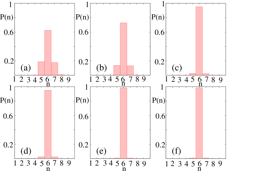
Figure 3: [Color Online]:The coordination number probability distribution at successive stages of freezing of the driven liquid, at driving forces $F_{x}=6(a),10(b),20(c),22(d),32(e)$ and $40(f)$ and with $v_{3}=6$. These forces correspond to the forces given in the configuration snapshots of Fig. 2.

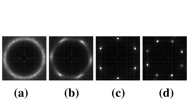
Figure 4: Structure factor $S({\bf q})$ for the plastic flow state (a), anisotropic hexatic phase(b), moving triangle (c) and moving square solid phases (d) at $v_{3}=6.0$ and $F_{x}=10,20,60$ and $140$ respectively. To obtain $S({\bf q})$, $50$ independent configurations were used. The structure in (d) reflects the presence of two misoriented square crystallites.

We show the evolution of the coordination number histograms of the system for the corresponding forces in Fig. 3. In the disordered state, 5-fold and 7-fold coordinated particles are roughly similar in number as expected. The number of particles with 5 and 7 fold coordination decrease with the drive (Fig. 3 (a),(b)). There appears to be a small intermediate regime where we see some clustering of these defects, as in (c) and (d). Finally, at much larger $F$, the number of non-hexagonal coordinated particles declines abruptly (Fig. 3 (e),(f)) and the system freezes into a triangular latttice. Similar observations hold for the case of scans in $F$ at larger $v_{3}$, with the difference that the ultimate large-force state is the flowing square lattice. Configurations in the “coexistence regime” obtained at much larger forces ($F\sim 100$ for $v_{3}=6$) are discussed separately in the sections which follow.

III.1 Pinned Phase:

For small $F$ the solid is pinned. In this regime, for $F<F_{c}$, there is no centre of mass motion at the longest times we simulate. We see transient motion in the initial stages of the application of the force, which then dies down once the system optimizes its location within the background of pinning sites. As $F$ is increased across the depinning threshold, there are long transient time-scales for motion to set inSengupta et al. (2007). These time-scales appear to diverge as the system approaches the transition, in agreement with expections concerning continuous depinning transitions. However, depinning appears to be hysteretic, on the length and time scales we consider i.e. the reverse path, from depinned to pinned states yields an abrupt transition between these statesSengupta et al. (2007, 2007). The depinned state just above the transition is inhomogeneous and undergoes plastic flowJensen et al. (1988a, b); Shi and Berlinsky (1991) consistent with earlier numerical work. For larger $F_{x}$ the velocity approaches the asymptotic behaviour $v_{CM}=F_{x}$.

The pinned phase is a phase with short-range order in both translational and orientational correlation functions. Correlations typically extend to about 4-8 interparticle spacings at the levels of disorder we consider. At non-zero noise strength, strictly speaking, we would expect an activated creep component to the motion. This presumably lies beyond the time scales of our simulation, given the relatively low temperatures ($T\ll T_{m}$) we work at.

III.2 Plastic flow phase

Upon increasing the force, we enter a regime of substantial plastic flowJensen et al. (1988a, b); Shi and Berlinsky (1991). This regime is one in which particle motion is extremely inhomogeneous. Similar plastic flow is seen in a large number of simulations of particle motion in a random pinning backgroundJensen et al. (1988a, b); Shi and Berlinsky (1991); Koshelev and Vinokur (1994); Faleski et al. (1996); Olson et al. (1998); Fangohr et al. (2001); Chandran et al. (2003); Kolton et al. (1999); van Otterlo et al. (1998). What is unusual here, however, is the strongly non-monotonic character of the plastic flow boundary, as illustrated in the phase diagram of Fig. 1. Note that the plastic flow phase boundary in the $F-v_{3}$ plane is largely independent of $F$ for small $v_{3}$. However, once the critical value of $v_{3}$ for the square-triangular transition is crossed, this boundary becomes a strong function of $F$, with the plastic flow region expanding considerably before it collapses again.

The structure factor $S(q)$ of the plastically moving phase (C) obtained in a narrow region just above the depinning transition consists of liquid-like isotropic rings, as shown in Fig. 4(a). For much larger values of $v_{3}$, the disordered, pinned phase appears to depin directly into the highly ordered moving square lattice phase, with no trace of a plastic flow regime. We have searched for tetratic phases, with algebraically decaying tetratic correlations in the vicinity of this depinning transition. However, no such phase is apparent in our numerics.

In the plastic flow regime, transport properties are noisy, reflecting the underlying highly disordered nature of the phase, in agreement with previous work on such plastic flow states in systems without competing phasesJensen et al. (1988a, b); Shi and Berlinsky (1991); Koshelev and Vinokur (1994); Faleski et al. (1996); Olson et al. (1998); Fangohr et al. (2001); Chandran et al. (2003); Kolton et al. (1999); van Otterlo et al. (1998). We see no evidence for a two-peak structure in the velocity distribution function, unlike some previous work, provided we average enough. Thus no particle is stationary over the full time-scales of our simulations.

III.3 Anisotropic Hexatic Phase

As $F$ is increased further, we encounter a narrow regime in which translational correlations are short-ranged while angle-averaged orientational correlations appear to decay as power laws. Within this phase the circular ring in $S(q)$ concentrates into six smeared peaks, as shown in Fig. 4(b). The presence of 6-fold order in the absence of the sharp Bragg-peaks associated with crystalline ordering suggests that this phase may have hexatic orientational order. We thus tentatively identify this phase as a driven hexatic, as shown in (D)Ryu et al. (1996); van Otterlo et al. (1998); the terminology “anisotropic” is justified in what follows. However, to strengthen this assignment, other possible assignments, such as to a coexistence regime known to plague similar analyses of hexatics in two dimensional systems, must be ruled outJaster (1999).

We compute the correlations of the hexatic order parameter for a very large system at varying values of $F$, as shown in Fig. 5, where $N=10000$. This figure displays the evolution of $g_{6}(r)$, as $F$ is varied across the phases $(C)\to(D)\to(E)$ at fixed $v_{3}=6$. We observe a sharp exponential decay of hexatic correlations in (C) and find that at the liquid to hexatic transition for $F\simeq 22$, the decay fits the universal behavior

$$g_{6}(r)\sim\frac{1}{r^{1/4}}$$ (15)

expected at the fluid hexatic transition in two-dimensional non-disordered fluids. This exponent is obtained in a relatively narrow range of forces. Our system sizes are comparable to typical sizes employed to observe a metastable hexatic phase in two dimensional melting of pure solids.

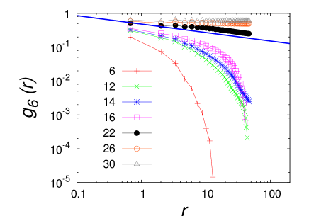
Figure 5: [color Online]: The hexatic correlation function $g_{6}(r)$ for $F=6,12,14,16,22,26$ and $30$, each averaged over 50 independent configurations of a $N=10000$ particle system at $v_{3}=6$. The solid line indicates the universal behavior $g_{6}(r)\sim r^{-1/4}$ at the liquid to hexatic transition.

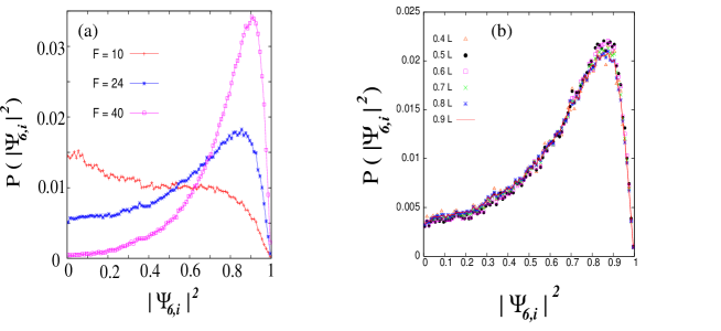
Figure 6: [Color Online:] (a)The distribution of the amplitude of the local hexatic order parameter $|\psi_{6,i}|^{2}$ over the system for $N=10000$ in the plastic ($F_{x}=10$), hexatic-glass ($F_{x}=24$) and moving triangular ($F_{x}=40$) regimes, with $v_{3}=6.0$ (b) Scaling of the distribution of $|\psi_{6,i}|^{2}$ deep in the hexatic regime for $F_{x}=26$, computed over fractions $0.4,0.5,0.6,0.7,0.8$ and $0.9$ of the simulation box length $L$, with $v_{3}=6.0$.

In Fig. 6(a), we compare the distribution of $|\psi_{6,i}|^{2}$ over the full system, for the plastically flowing, moving triangular and the intermediate hexatic-glass regimes. The figure illustrates that in the liquid/plastic regime ($F=10$), the distribution is primarily governed by non six-fold coordinated particles. In the high driving force regime ($F=40)$, six-fold coordinated particles contribute in main. This raises the question of whether the intervening ‘hexatic’ regime we observe in terms of $S({\bf q})$ and the correlation of the hexatic order parameter $g_{6}(r)$ at $F=24$, is truly hexatic or defined by a coexistence of the ‘solid’ and ‘disordered’ phases. If configurations resemble those at solid-fluid coexistence, the distribution would be expected to be a sum of the disordered, relatively ordered and interface distributions (weighted with their relative areas).

To settle this issue we investigate the dependence of the distribution of $|\psi_{6,i}|^{2}$ on the size of the system. The distribution is obtained by dividing the system into a number of blocks and computing the distribution of $|\psi_{6,i}|^{2}$ within each block for every configuration. In this way, information over many length scales can be obtained from the same set of configurations. This provides us with the distribution of $|\psi_{6,i}|^{2}$ for various fractions of the total system.

We find, as shown in Fig. 6(b), that apart from finite size effects, there is not much difference between the distributions. Also, the distributions for the two largest systems, viz. $0.8L$ and $0.9L$ ($L$ being the size of the simulation box), coincide to within statistical errors. In the case of two-phase coexistence one would expect a strong size dependence when the size of the blocks is comparable to the size of the phase separating clusters. These observations rule out two-phase coexistence, at least of the conventional kind, as an explanation for the long orientational correlations obtained on circular averaging.

As we show below, a more detailed characterization of this phase yields the following results: Long-range order in orientation is always present in the direction of drive, while remaining short-range in the perpendicular direction. When averaged over all orientations, the resulting function appears power-law-like over 2-3 decades i.e. over length scales addressed in virtually all simulations so far. Thus, while we call the intervening phase as the “anisotropic hexatic”, we diverge sharply from previous work in our claim that the true phase is never a true hexatic in the real sense, since it always has long-range order in the drive direction. We conclude that the apparent hexatic correlation arises, in fact, as an artefact of circularly averaging a very anisotropic correlation function, with qualitatively different decays in the longitudinal and transverse directions.

III.3.1 Analogy to the XY model

The power-law decay of orientational correlations shown in Fig. 5, taken together with the scaling of $|\psi_{6,i}|^{2}$ suggests that the driven system in the vicinity of $F=22$ might best be described as a hexatic, with power-law correlations in the local orientation but short-range translational order. Such a state is analogous to the low-temperature phase of the 2-dimensional XY model, where the Mermin-Wagner theorem rules out long-range order at any finite temperature but vortex-like excitations responsible for the transition to the disordered phase exist chiefly as bound vortex-anti-vortex pairs. However, the presence of the drive direction introduces an anisotropy into the system. The consequences of this anisotropy have not, to the best of our knowledge, been explored in previous studies of putative hexatic phases in driven disordered solidsRyu et al. (1996).

In our studies, we have been motivated by an analogy to the physics of the XY model in an applied field, specifically by the intriguing possibility that the drive might play a role equivalent to that of the magnetic field in the XY model. Renormalization group studies Fertig (2002) of the 2-dimensional XY model in an external magnetic field with Hamiltonian,

$$\mathcal{H}_{XY}=\sum_{i,j}J_{ij}s_{i}s_{j}\cos(\theta_{i}-\theta_{j})-h\sum_{i}s_{i}\cos(\theta_{i})$$ (16)

where the external field $\bf h$ points along the positive $x$-axis, indicate three distinct phases. These are a linearly confined phase, a logarithmically confined phase and a free vortex phase obtained as the temperature is gradually increased. Vortex-antivortex pairs at low temperatures are linearly confined by a string of overturned spins. With increasing temperature these strings participate in a proliferation transition, but vortices still remain confined due to a residual logarithmic attraction. As the temperature is further increased, the vortices overcome this attraction and are finally deconfined.

Since the external field breaks rotational symmetry, the magnetization is non-zero in all the three phases. Further, the free energy is argued to be smooth; thus the distinction between phases can only be found in the structure and distribution of topological defects. The correlation function $\langle\cos(\theta_{i})\cos(\theta_{j})\rangle$ is then predicted to saturate to a constant value ($b$, say) for $|{\bf r}_{i}-{\bf r}_{j}|\to\infty$. This constant $b\propto h^{2}$ since the order parameter ($\cos(\theta_{i})$) couples linearly to the field $h$. On the other hand, the correlation function $\langle\sin(\theta_{i})\sin(\theta_{j})\rangle$ which corresponds to spin fluctuations in the direction transverse to the applied field (see Eq. (6.6)), is predicted to show an exponential decay in all the three phases.

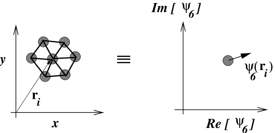
Figure 7: Mapping to the XY model : local hexagonal configuration around the particle $i$ (diagram on left) may be analyzed in terms of the phasor $\psi_{6}({\bf r}_{i})$ represented as a spin situated at ${\bf r}_{i}$ (diagram on right).

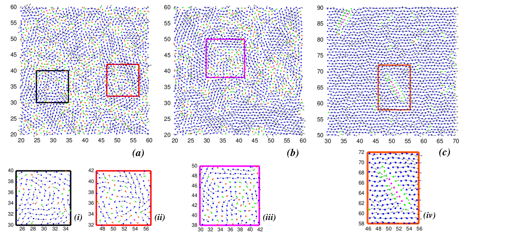
Figure 8: [Color Online]: Typical orientation of the ‘hexatic-spins’ (see text) associated with particles in the liquid (a), anisotropic-hexatic (b) and triangular (c) phases, at the driving forces $F_{x}=10,24$ and $40$ respectively. The boxes in (a), (b) and (c) are expanded in (i) and (ii) (corresponding to the configurations boxed in (a)), in (iii) (corresponding to the configuration boxed in (b)) and (iv), corresponding to the boxed configuration in (c), to enable an easier visualization of spin configurations. The colors correspond to local coordination, $n=6$ (blue), $5$ (green), $4$ (magenta) and $7$ (orange). Note the presence of extended defects in the ordering shown in (c), associated with “strings” with local square symmetry. In all the three pictures only a part of the simulation box is shown for the sake of clarity and the configurations are obtained for $v_{3}=6$.

III.3.2 Quantifying Local Orientational Order

To test this possibility, we must map local orientational order to an appropriate XY-like two-dimensional vector from which defect structures can be extracted. This is done through the local hexatic order parameter, $\psi_{6,i}\equiv\psi_{6}({\bf r}_{i})$, defined earlier. It is convenient to identify this local quantity (a phasor) with a ‘hexatic-spin’ with components $Re[\psi_{6,i}]$ and $Im[\psi_{6,i}]$, thus mapping local geometrical order to a soft-spin XY degree of freedom.

We illustrate this mapping from the local orientations of particles in real space to XY spins in Fig. 7. Unlike in the XY model, such hexatic spins are not attached to a fixed lattice but associated with the moving particles. They thus encode important information concerning the equal-time orientational correlations in the driven system. Fig. 8 shows real space configurations of the particle system with associated hexatic spins at various values of $F$, illustrating the variety of associated spin configurations present in this mapping.

These configuration maps enable the identification of topological defects in the ordering in the associated XY model. Note the presence of locally aligned regions as well as vortex-like excitations of strength 1 and 1/2. Qualitatively, we find that in both the disordered liquid phase and the anisotropic hexatic phases, vortex configurations in such spin configurations appear to have little correlation with each other, suggesting that they may be either unbound or relatively weakly bound at best (see Fig. 8 (a) and (b)); the boxed regions of these figures as indicated are expanded in Fig. 8(i) and (ii) for (a) and in (iii) for (b). However, we have not been able to establish a quantitative distinction between the disordered liquid phase and the anisotropic hexatic phase using our simulation data.

Some quantification is, however, possible for larger forces, in the flowing triangular phase, (Fig. 8 (c)), where defects in the ordering appear to be associated with strips, or strings, of defect. In this case, the defect is locally a solid with square symmetry. (An expanded plot of the boxed region in Fig. 8(c) is shown in (iv), illustrating the one-dimensional character of the defect). We expect that such defects should be linearly bound, with an energy proportional to the length of the strip. The binding energy in the latter case should be proportional to a non-equilibrium analog of a surface tension between the square and the triangular crystal. This argument is supported by calculations of the moment of inertia tensor of the set of particles which belong to such a defect, averaged over configurations which contain such defects. The largest eigenvalue ($\lambda_{>}$) of this tensor measures the length of these extended string-like defects. In Fig. 9 we show the probability distribution $P(\lambda_{>})$ at a few different values of the external drive. It is clear that within the intermediate force regime, the distribution is exponential, implying that the energy for these excitations scale linearly with their size. These string like excitations align preferentially along the crystallographic axes of the surrounding triangular lattice. As the force is increased, these defects offer nucleation sites for square crystals which are less anisotropic. The probability distribution then ceases to be linear in $\lambda_{>}$, leading to the long tail in the data shown in Fig. 9 at $F=110$ .

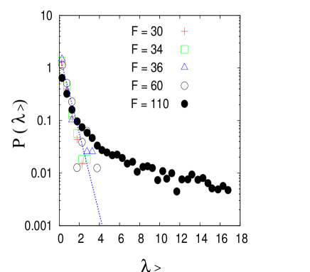
Figure 9: [Color Online]:Probability distribution of the largest eigenvalue $\lambda_{>}$ in a semi-logarithmic scale for external forces $F=30,34,36,60$ and $110$. It is clear that for all but the largest force, the probability distribution is exponential showing that the energy of string-like excitations within the triangular phase is linear with size. For the largest force which is inside the coexistence region (see text), the probability distribution decays slower than an exponential.

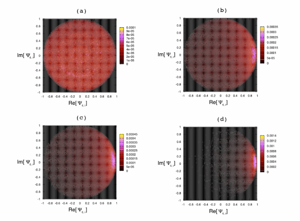
Figure 10: [Color Online]: Probability distribution of the ‘hexatic-spin’ phasors for forces $F_{x}=8$ (a), $22$ (b), $24$ (c) and $40$ (d). The plane of the Argand Diagram within the area enclosed by the points $(-1,-1)$, $(1,-1)$, $(1,1)$ and $(-1,1)$ is subdivided into $200\times 200$ square boxes (of width $0.01$). The sum of the probability distribution over these boxes is normalized to unity.

Fig. 10 shows the probability distribution of the ‘hexatic-spin’ phasors for forces $F_{x}=8$ (a), $22$ (b), $24$ (c) and $40$ (d). While Fig. 10(a), obtained within the plastic flow phase, appears to have a uniform distribution of hexatic spins with angle, Figs. 10(b), (c) and (d) display substantial non-uniformity in this distribution. Note the following feature of Fig. 10(c): The mapped spins tend to overwhelmingly point along the drive direction in the flowing triangular state. This should be contrasted with the fact that the corresponding distribution function for the X-Y model in zero external field is isotropic across the disordered to quasi-long-range-ordered transition, peaking below it at $|\Psi_{6}|\neq 0$, a value independent of the phase angle, in a finite system. This indicates that orientational order in our problem is strongly biased by the drive $F$, if $F$ is sufficiently large.

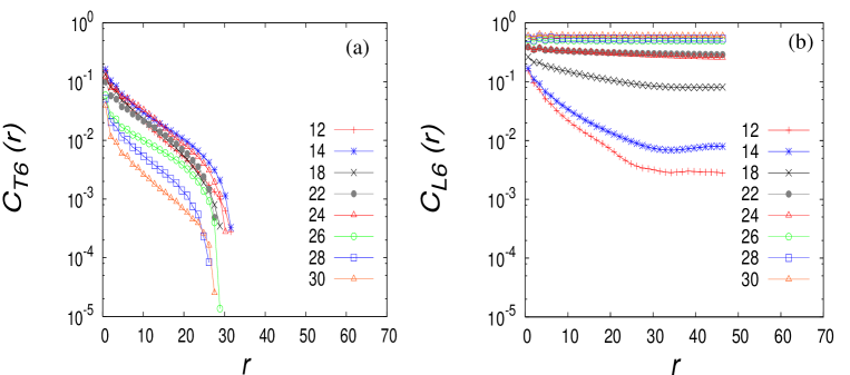
Figure 11: [Color Online]: (a) The correlation functions $C_{T6}(r)$ plotted for a range of force values $F_{x}=12,14,18,20,22,24,26,28$ and $30$ and for $v_{3}=6.0$. Note the generic exponential decay obtained. (b) The correlation function $C_{L6}(r)$ (see text) plotted for a range of force values $F_{x}=12,14,18,20,22,24,26,28$ and $30$. in Ref.Fertig (2002).

The probability distribution of the hexatic-spins in the complex Argand plane formed by the Re$[\psi_{6,i}]$ and Im$[\psi_{6,i}]$ axes clearly describes how the external symmetry-breaking field ($F_{x}$) builds up anisotropy in the our system, thus ordering the spin orientations. At low drive, the anisotropy is masked by disorder-induced fluctuations at the scale of our simulation box. As such fluctuations are increasingly suppressed at higher drive values, the system appears to organize into a coherently moving lattice structure whose principal axes are biased by the force.

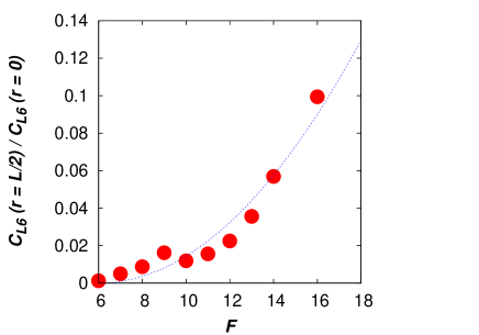
Figure 12: [Color Online:] The constant part in the angular correlation function along the drive direction goes quadratically with the driving field strength above $F_{c}$ as predicted by Fertig et al.Fertig (2002). The data points (circles) are for $v_{3}=6.0$ and the dashed line is a guide to the eye.

The spin-spin correlation functions in our model, Fig. 11(a) and Fig. 11(b), obtained via the correlation functions $C_{L6}(r)$ (longitudinal) and $C_{T6}(r)$ (transverse), correspond to the local quantities Re$[\psi_{6,i}]$ and Im$[\psi_{6,i}]$. They are

$$C_{L6}(r)=\langle Re[\psi_{6}(0)]Re[\psi_{6}(r)]\rangle$$ (17)

$$C_{T6}(r)=\langle Im[\psi_{6}(0)]Im[\psi_{6}(r)]\rangle$$ (18)

In all the phases (C), (D) and (E) of Fig. 1, the orientational correlation function $C_{L6}(r)$ saturates asymptotically, as expected, to a constant. In phase (D), such saturation is obtained only in the drive direction. The transition from phase (D) to phase (E), when triangular translational order increases continuously with $F_{x}$, appears to be smooth. The correlation function $C_{T6}(r)$ decays exponentially in all the three phases.

Note that our mapping for orientational order and its correlations in the moving state is free from any underlying lattice effects, in contrast to earlier studies of the XY model in a field. Therefore, any anisotropy reflected in the spin distribution (see Fig. 10) or their correlation functions reflects an intrinsic property of the particular driven phase. The quadratic dependence of the asymptotic saturation value of $C_{L6}(r)$ on the applied field $F_{x}$ within the fluid (plastic flow) regime, as predicted by this intuitive mapping, is shown in Fig. 12.

The results presented here address one fundamental issue in the literature on orientational order in driven disordered states, in particular the question of whether a quasi-long-range ordered phase, the “hexatic” can exist. We show here conclusively that it cannot. What exists is an unusual intermediate state which possesses long-range orientational order in the direction singled out by the drive whereas orientational order decays exponentially in the transverse direction.

III.4 Phases at Large Force: Square, Triangular and Coexistence

What happens at still larger force values depends on the value of $v_{3}$. For small $v_{3}$, the system transits directly from anisotopic hexatic glass to triangular moving crystal. The Bragg peaks sharpen into sharp Bragg spots with six-fold symmetry. At intermediate values of $v_{3}$, the system appears to undergo an unusual transition into what we term a “coexistence phase”, discussed in more detail below. In this phase, the system has both triangular and square domains and interconverts between them over a broad distribution of time-scales. Inspection of configurations suggests an analogy to equilibrium phase coexistence with a large, heterogeneous distribution of domain sizes of triangular and square regions, although this is an explicitly non-equilibrium system.

At larger values of $v_{3}$, the coexistence regime appears bounded. However, the disordered, plastic flow regime is observed to expand. At these values of $v_{3}$ the system undergoes a direct transition into the square phase. For much larger $v_{3}$, the phase boundary between plastic and square phases collapses again with increasing $v_{3}$, reducing the extent of the plastic regime. In this large $v_{3}$ regime, the system depins discontinuously and elastically from a pinned to moving square crystal with no intervening plastic flow phase that our numerics can resolve. The plastic flow regime (C), as well as that of the hexatic glass (D) expands at larger $v_{3}$ due to the frustration of local triangular translational order by three-body interactions. On further increasing $F_{x}$, the structure obtained depends on the value of $v_{3}$: for low $v_{3}$ the final crystal is triangular (E) whereas for large $v_{3}$ it is square (F). We assign these states through a study of the structure factor $S(q)$, as well as the coordination number probability distributions shown in Fig. 3, observing that the slighly smeared six-fold coordination of the hexatic glass consolidates into sharp Bragg-peaks across the transition into the ordered states, as shown in Fig. 4.

III.5 The Coexistence phase

For intermediate $v_{3}$ and $F$, the system exhibits a remarkable “coexistence” regime (G) best described as a mosaic of dynamically fluctuating square and triangular regions. From a direct calculation of the structure factor we see the simultaneous appearance of peaks corresponding to hexagonal and square orderSengupta et al. (2007). The intensity of the peaks from the hexagonal and square phases are comparable.

As $F$ is increased, clusters of $4$-coordinated particles grow in size. The evolution of the configuration with increasing force is shown in Fig. 13, which illustrates the square-triangle domain mosaic characteristic of the coexistence regime. The $6$-coordinated regions decrease in size and the dynamics of the interfacial region - with predominantly $5$-coordinated particles and with a few isolated $7$-coordinated particles - shows enhanced and co-ordinated fluctuations. Real space configurations (Fig. 13) exhibit islands of square and triangular coordination connected by interfacial regions with predominately 5 coordinated particles. The configuration, as viewed in the co-moving frame, is extremely dynamic, with islands rapidly interconverting between square and triangle. This interconversion has complex temporal attributes.

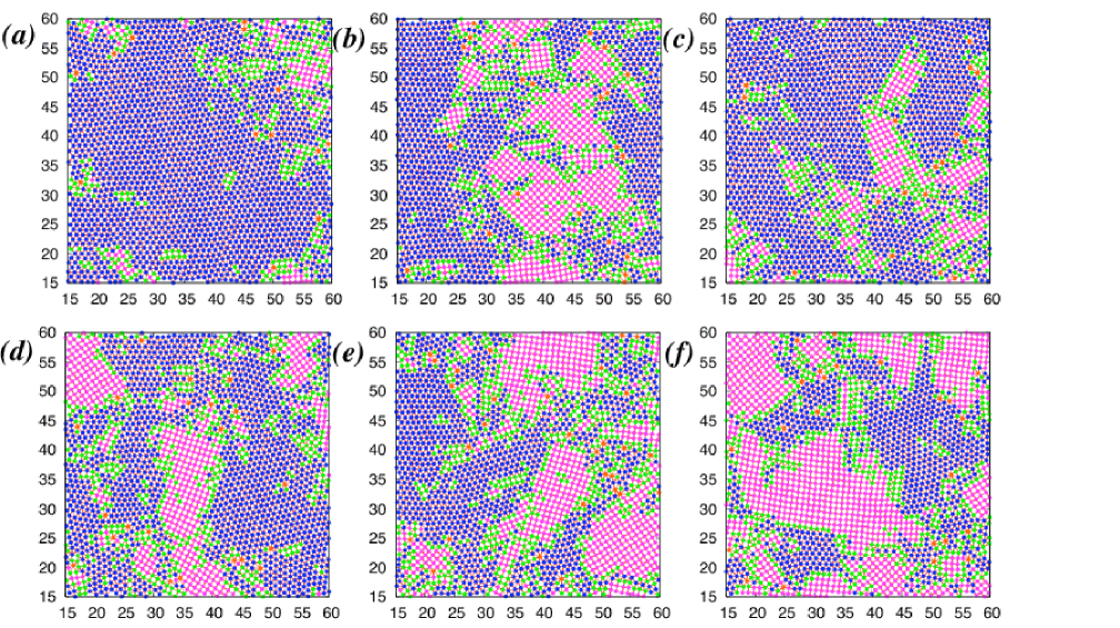
Figure 13: [Color Online:] Evolution of configurations showing square-triangle coexistence with increasing force $(a)F=90,(b)95,(c)100,(d)105,(e)110,$ and $(f)115$, together with the computed Delaunay mesh. The particles are colored according to the number of neighbors n = 4 (magenta), 5 (green), 6 (blue) and 7 (orange). Particles with coordination 5 are present mainly in the interfacial region while those with 7 are associated with isolated dislocations.

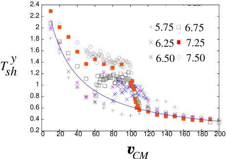
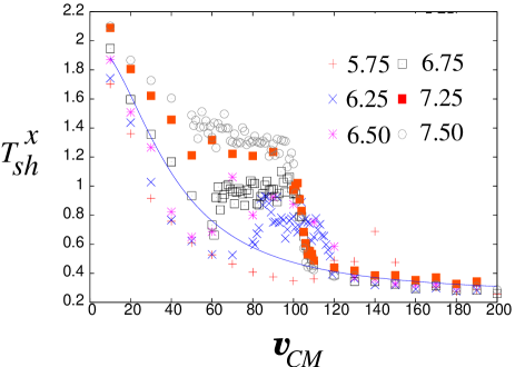
Figure 14: [Color Online]: The shaking temperatures in the transverse (top) and drive (bottom) directions ($T_{sh}^{y}$ and $T_{sh}^{x}$) for different $v_{3}$ as a function of the centre of mass velocity ($v_{CM}$), showing the quantity is almost independent of $v_{3}$ except in and around the coexistence regime, due to effects of fluctuation.

As substrate randomness is averaged out due to the motion of the particles, the shaking temperature of the system can reasonably be expected to decrease. This is reflected in the decrease of the width in velocity component distributions. The “shaking temperature” predictions of Koshelev and Vinokur, would indicate a $\sim 1/v$ and $\sim 1/v^{2}$ nature of the fall in the transverse and drive directions respectively. Our results for $T^{\nu}_{sh}$ are in agreement with this prediction outside the coexistence regime.

We find, as shown in Fig. 14, that $T^{\nu}_{sh}$ is nearly independent of $v_{3}$. However, within the coexistence regime, $T^{\nu}_{sh}$ behaves non-monotonically. Typically, for a particular disorder configuration and for $5.5<v_{3}<8.5$, $T^{\nu}_{sh}$ appears to increase sharply at a well defined $F_{x}$, signifying the start of coexistence. Within G, $T^{\nu}_{sh}$ remains high but drops sharply at the upper limit of G, to continue to follow the interrupted KV behavior. This anomalous enhancement of fluctuation magnitudes provides strong evidence for a genuine coexistence phase, since increasing the driving force would be expected to reduce current noise monotonically once the system depins, as observed in all previous simulation work on related models Faleski et al. (1996); Fangohr et al. (2001). The limits of the coexistence region, though sharp for any typical disorder realization, vary considerably between realizations.

Clusters within the coexistence state appear through a nucleation and growth mechanism, as modified by the anisotropy induced by the presence of the drive. Fig. 15 shows that for a particular disorder realization at a force $F_{x}=98$, a nucleus of square region appears which grows with time. In all the disorder realizations we studied, the square nucleus first formed in the hexagonal phase is anisotropic and elongated along the transverse direction (Fig. 15), a consequence of the fact that the drive introduces a preferred direction into the system.

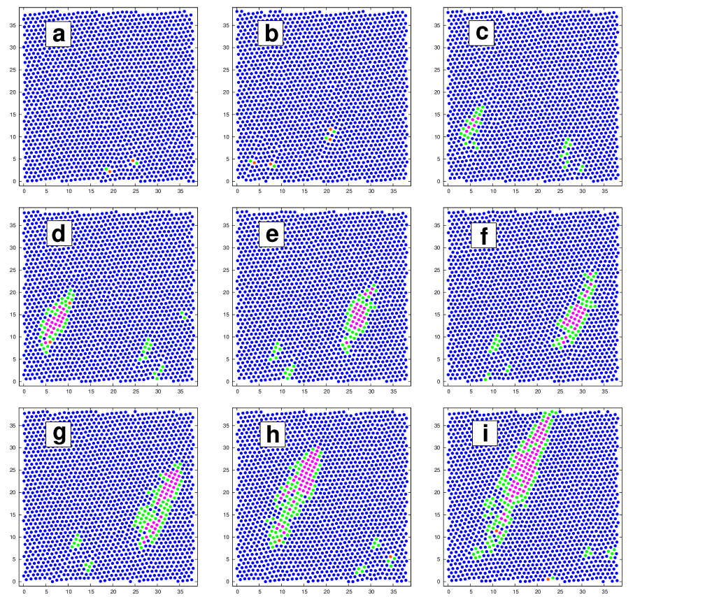
Figure 15: [Color Online:] Dynamical nucleation of a square defect against a triangular background, shown for $F=98$, $v_{3}=6.0$ and at $TimeSteps=60\times 10^{3}(a),70\times 10^{3}(b),80\times 10^{3}(c),84\times 10^{3}(d),86\times 10^{3}(e),90\times 10^{3}(f),94\times 10^{3}(g),96\times 10^{3}(h),10^{5}(i)$

Square clusters in the coexistence regime tend to be less anisotropic compared to the elongated string-like defects of square within a triangular background obtained at smaller force values. This can be seen from Fig. 16 which plots the distribution of angles made, with respect to the drive direction, by the principal direction of the square nucleus, corresponding to the larger eigenvalue of the moment of inertia tensor. For small $F$, the distribution peaks around $\theta=\pm 60^{\circ}$, indicating that the square nucleus forms preferentially at a $60^{\circ}$ angle with respect to the drive. For forces within the coexistence regime, however, the distribution of this angle is smooth and has no sharp peaks, concomitant with the shape of the nucleus becoming more isotropic.

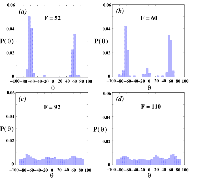
Figure 16: [Color Online:] The distribution of the angle made by the major principal axis (the eigenvector corresponding to the eigenvalue $\lambda_{>}$) of the square islands within a triangular background, computed for different values of the driving force $F$. The force values are (a) F = 52, (b) F = 60, (c) F = 92 and (d) F = 110, with $v_{3}=6$.

III.5.1 Noise in the Coexistence Regime

The interconversion between square and triangular regions leads to complex spatio-temporal behavior. To demonstrate this, we compute the power spectrum of fluctuations of the particle current. We first obtain the statistics of the number of particles crossing an imaginary line parallel to the transverse ($y$) direction per unit time, per unit length of the line for a particular force ($F_{x}$) value. The power spectrum $S_{flux}(f)$ is the Fourier transform of the auto-correlation function of this time series of particle flux, averaged over different choices of the position of the imaginary line and over different choices of the time slots of observation. Considerable statistics were taken to ensure that all quantities were well averaged. About $5$ different choices of the position of the transverse imaginary line were taken, in addition to $20$ different choices of time slots. Averaging is performed over a large span of simulation time steps ($\sim 10^{9}$).

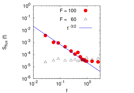
Figure 17: [Color Online:] The power spectrum $S_{flux}(f)$ of current fluctuations in the moving triangle phase (open triangles $F_{x}=60$) and in the coexistence region (red circles $F_{x}=100$), logarithmically binned and plotted for a range of frequencies below the washboard frequency. Current fluctuations in the coexistence region are enhanced, also showing a $1/f^{3/2}$ decay in the low frequency range.

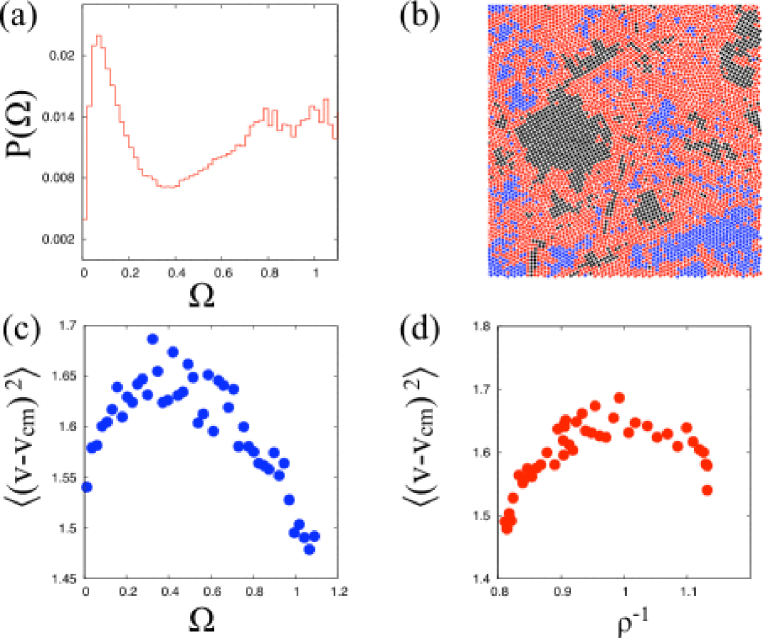
Figure 18: [Color Online:] (a) Probability distribution of the bond angle order parameter $\Omega$ (see text) in the coexistence regime. The peak at low value of $\Omega$ corresponds to the square phase. The series of peaks at high $\Omega$ values all correspond to various combinations of bond angles in the (disordered) triangular phase. The interfacial region has $\Omega$ corresponding to the first dip in the curve. (b) Illustration of the spatial distribution of $\Omega$ values as stated in (a) $\Omega<0.2$ (square) are black, those for $1.3>\Omega>0.2$ are red (interface) and those for $\Omega>1.3$ are blue (triangle). (c) The fluctuation of the local velocity about the centre of mass value $<(v-v_{cm})^{2}>$ plotted against $\Omega$. It is clear that the fluctuations are largest for the particles in the interfacial region. (d) The fluctuation of the local velocity as a function of the local volume per particle.

Our results are summarized in Fig. 17 for two values of $F_{x}$. For $F_{x}=60$, when the system is in the moving triangular phase, $S_{flux}(f)$ is, to a large extent, featureless and flat, except for large $f$ where effects due to the streaming of the entire system become important. In contrast, for a high force $F_{x}=100$, when the system is within the coexistence phase, we obtain a $1/f^{\alpha}$ regime, with $\alpha\simeq 1.5$ in $S_{flux}(f)$ over about a decade. In addition the particle current fluctuations remarkably enhanced by 3-4 orders of magnitude in the coexistence phase as compared to the triangular regime.

III.5.2 Origins of Noise in the Coexistence Regime

To investigate the origins of the noise in the coexistence regime, we define the local quantity

$$\Omega_{i}=\sum_{j,k}\sin^{2}(4\theta_{ijk}),$$ (19)

where the summation is over a defined region ($r<r_{0}=1.2\sigma$) surrounding a particle i. Here $\theta_{ijk}$ is the bond angle between particle $i$ and $j$ and $k$. We choose particles $j$ and $k$ such that they are all within a specified cutoff radial distance from particle i.

Fig. 18(a) displays the probability distribution of $\Omega\equiv\Omega_{i}$ for a state in the coexistence region. There are two prominent peaks. The peak for small values of $\Omega$ corresponds to the square lattice ($\Omega=0$ for the ideal square crystal), whereas the peak at higher values of $\Omega$ corresponds to the triangular structure. Intermediate values of $\Omega$ are obtained for particles at the interface between square and triangle. Fig. 18(b) shows a snapshot of the system in the coexistence region with particles color coded according to their value of $\Omega$.

We next examine the fluctuations of the velocity about the average value $\langle(v-v_{cm})^{2}\rangle$ as a function of the local coordination. In Fig. 18(c) this is plotted as a function of $\Omega$. We see that velocity fluctuations are larger in the interfacial region. Further, Fig. 18(d) shows a plot of the local volume per particle as a function of the velocity fluctuations, showing that the relatively lower density of the interfacial region (due to the presence of a large concentration of defects) causes it to fluctuate more than the rest of the solid. The rapid fluctuations of the interface also results in rapid interconversion between square and triangular coordinated particles and leads also to enhanced fluctuations in the coordination number. Since the driven solid is elastically constrained to move as a whole in the direction of the drive without gaps or cracks, this sets up strong correlations among the particle trajectories. Such correlations are ignored in the theory of the shaking temperature of Koshelev and Vinokur.

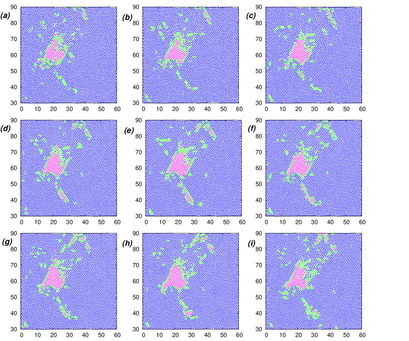
Figure 19: [Color Online:] Configuration snapshots arising from a quench to zero force of a randomly chosen configuration within the coexistence regime, at time steps (a) 0, (b) 4$\times 10^{3}$, (c) $10^{4}$, (d) 5 $\times 10^{4}$, (e) $10^{5}$, (f) $2\times 10^{5}$, (g) $3\times 10^{5}$, (h) $5\times 10^{5}$, and (i) $9\times 10^{5}$, with $v_{3}=6.0$. The system size is N = 10000.

IV Dynamical Coexistence and Peak Effect Anomalies

In this section, we turn to a possible application of this model, in the context of experiments on transport anomalies associated with peak effect phenomena in the superconducting mixed phase. To recapitulate, the peak effect refers to the sharp increase in the critical current $j_{c}$ in the mixed phase of a disordered type-II superconductor close to H${}_{c2}(T)$. This critical current is thus a non-monotonic function of $T$ (or $H$, depending on which is varied experimentally), since it decreases steadily from its low temperature value till the onset temperature $T_{o}$ of the peak effect, from whence it increases sharply over a small temperature range to its maximum value, obtained at temperature $T_{m}$. As $T$ is raised still further, the critical current collapses again, to reach zero in the normal state. The temperature interval [$T_{0},T_{m}$] in which the critical current rises anomalously is the peak effect regime. This regime is dynamically anomalous, displaying: (i) large current noise amplification at low frequency, (ii) a $1/f$ spectrum of current fluctuations, which is very non-Gaussian, (iii) a “fingerprint” effect in which apparently random spikes in the differential resistivity as a function of drive are retraced as the drive is decreased, (iv) a history-dependent dynamic response (v) a memory of direction, amplitude and frequency of applied currents, (vi) a strong suppression of ac response by a dc bias as well as a variety of other behaviourBhattacharya and Higgins (1993, 1994, 1995); Marley et al. (1995); Merithew et al. (1996); Henderson et al. (1996); Ghosh et al. (1996); Ravikumar et al. (1998); Banerjee et al. (1998, 1999, 2001); Henderson et al. (1998); Xiao et al. (1999). A very large number of experiments probing such anomalous behavior, including all those referenced above, are transport-based, thus serving as probes of the dynamics of vortices within this narrow region of parameter space.

Interpretations of these phenomena are largely phenomenological. One particularly influential proposal considers an underlying order-disorder transition “contaminated” by sample surfaces or “edges”. Such surfaces, with associated surface barriers for vortex entry, provide an entry point for vortices driven into flowBeidenkopf et al. (2005). The surface should provide an intrinsically more disordered environment for vortices than the bulk, particularly in fairly pure samples where $j_{c}$ is low. Thus, vortices might be expected to enter through the boundaries in a highly disordered state, only to anneal in the nearly pure bulk, when a current is applied across the sample. This spatial separation of disordered and ordered states and the slow annealing of one into the other is argued to be the central feature underlying the anomalous behavior seen in the peak effect regime. Magneto-optic imaging via Hall bar arrays support the surface contamination scenario. However, such methods do not access the dynamics of annealing and phase transformations directly. Much recent work appears consistent with a bulk coexistence of disordered and ordered phasePasquini et al. (2008), while decoration experiments see a “multi-domain” structure in the peak effect regimeMenghini et al. (2002); Fasano et al. (2002), as proposed in Refs. Menon (2001, 2002a, 2002b) and accessed indirectly in Refs. Divakar et al. (2004); Menon et al. (2006). For related simulations, see Ref. Moretti et al. (2005).

The edge contamination scenario implicitly assumes that the underlying order-disorder transition is unaffected by the drive, serving only to provide a background to the annealing process. However, in a generic driven system, the possibility that the drive has more non-trivial effects must be expected. In particular, the drive may alter the very nature of the driven bulk, stabilizing dynamical states that are truly non-equilibrium in character, as illustrated in the simulations discussed above.

A beautiful recent experiment (Ref. Marchevsky et al. (2001)) performs a variant of scanning probe microscopy, using a mounted local Hall probe. The probe is sensitive to variations in the local magnetic induction averaged across a mesoscopic scale of around a micron. The system is tuned across the peak effect regime and then perturbed weakly through a low-amplitude ac field applied from below the sample. The Hall probe, placed above the sample and linked, though lock-in techniques to the frequency of the ac perturbation, records a local susceptibility, indicative of pinning response, as a function of space and integrated over the thickness of the sample. The spatial resolution is limited by the size of the Hall probe, typically of the order of a micron or so in size.

As parameters are varied across the peak effect, these experiments see a remarkable coexistence between a strong pinning regime and a weak pinning regime. A complex interface is seen between these coexisting states with a dynamics which is exquisitely sensitive to the field and the disorder, Such coexistence is also a feature of other phenomenological approaches to this problem, which address transport measurements. Locally more disordered regions of the sample appear to nucleate more stable regions of strong pinning whereas small variations of the applied field cause large changes in the inhomogeneous pinning pattern. However, the complex geometry of the coexisting regimes appears largely stable if the temperature and field are fixed, suggesting that thermal fluctuations are not dominant. While vortices entering from the sample boundaries do appear to contribute to this dynamics in no small measure, there is significant evidence for non-trivial dynamics in the bulk, with regions of strongly pinned phase being nucleated far from any boundary. Thus, these experiments point to a more active role for the bulk than envisaged in the boundary injection scenario. In this context, the authors of Ref. Marchevsky et al. (2001, 2002) have specifically argued that the complex topology of the two-phase interface should be largely responsible for the history dependence seen in the experiments.

How are these remarkable observations related to the model we study here? We suggest that the link is the emergence of a self-organized, disorder-stabilized, dynamically sustained drive-induced coexistence phase seen both in the experiments and in simulations of our model system. The similarities between the two are striking: First, the coexistence itself. Both the experiments and our simulations here provide incontrovertible evidence for dynamical states in driven disordered systems which resemble phase coexistence at equilibrum phase transitions, with the added complication of spatial inhomogeneities due to quenched disorderValenzuela and Bekeris (2000); Pasquini and Bekeris (2006); Pasquini et al. (2008); Jang et al. (2009). Reasoning from the experiments, the complex interconversion of one phase into the other and the spatially inhomogeneous character of the dynamics is the hallmark of vortex dynamics within the peak effect regimeMarchevsky et al. (2001). This is precisely the situation which obtains in the simulations. As pointed out in the previous section, what is unusual about the coexistence regime is that the strong disorder-induced fluctuations seen and manifest in all the dynamic properties we measure are obtained above the depinning transition, surviving even at large values of the applied force.

Second, the coexistence seen in the experiments is very disorder-sensitiveMarchevsky et al. (2001); Jaiswal-Nagar et al. (2006). In experiments, this is manifest in terms of the complex structure of differentially pinned regions in the sample, presumably reflecting a non-trivial pinning landscape. We see similar dynamical behavior within the coexistence regime, with the structure at fixed drive influenced by the underlying microscopic disorder and sensitive to even marginal changes in the pinning. Thus, the nature of inhomogeneities connected to dynamical phase coexistence in this model as well as in the experiments appears to be dictated primarily by the underlying disorder.

Third, the slow dynamics and long relaxation times seen in the experiments, reflecting the complex dynamics of the interface separating the regimes of different pinning strength, is seen in our simulations as wellHiggins and Bhattacharya (1996); Thakur et al. (2005). In our simulations, if the drive is switched off and the system allowed to anneal, the nuclei of one phase within the other live anomalously long, suggesting that the dynamics has stabilized long-lived metastable states, precisely as seen in the experiments. In Fig. 19 we show the dynamics of a square nucleus within a triangular background, extracted from a typical configuration within the coexistence regime, when quenched to zero drive. Far from vanishing over a short time scale, the nucleus appears to be remarkably stable out to the longest time scales accessed in our simulations, providing evidence that the metastability exhibited in the coexistence regime survives even after the drive is turned off. These are reflected in the memory experiments, in which the removal of the driving transport current essentially appears to freeze the system into a metastable state from which it only recovers upon a reapplication of the drive.

Fourth and finally, the noise spectra within the coexistence regime, including the anomalously large noise and the power-law fall-off with a $1/f^{\alpha}$ spectrum is a prominent feature of the peak effect regime. Experiments see a power-law falloff, with $1\leq\alpha\leq 2$, as well as a substantial enhancement in noise power of a few orders of magnitudeMarley et al. (1995); Merithew et al. (1996). The substantial non-Gaussian features in the noise, as obtained in Ref. Merithew et al. (1996), indicate that a small number of fluctuators contribute; it is tempting to assign these to a few large domains which fluctuate collectively within the coexistence regime, as suggested by the simulations.

The edge contamination scenario assumes that the drive in the bulk anneals the disordered vortices injected across the boundaries into the smoothly flowing state. In contrast, we show that in the vicinity of an underlying transition, the bulk flowing state is generically inhomogeneous and dynamically non-trivial, thereby questioning this basic assumption. We believe that the edge contamination scenario should apply, more immediately, close to but away from the peak effect regime, where the drive in the bulk acts solely to smoothen flow, precisely as seen in a recent experimentMohan et al. (2009).

We stress that the system we simulate is far from a literal translation of the vortex system. It lacks the $K_{0}(r/\lambda)$, (with $\lambda$ the penetration depth), interactions of vortex lines, which can become fairly long-range if $\lambda$ is large. In our simulations we drive transitions between the two different pure system phases by varying a parameter $v_{3}$, whereas these transitions are density or temperature driven in the classic scenario of the peak effect in vortex systems. (The underlying order-disorder transition in the vortex system is likely related to a melting-like transition, at least for small $H$ and for temperatures close to $T_{c}$ and not a structural transition between two crystalline phases as in our modelMenon (2002b).) The experiments are in three dimensions, whereas our simulations are two-dimensional. Our system shows very little variation in the depinning force close to the transition, and thus no apparent peak effect. (It is known, however, that factoring in the temperature dependence of the coherence length $\xi$ and $\lambda$ is essential to obtain a peak effect in two-dimensional simulationsChandran et al. (2003).)

For these, as well as other reasons, our proposal for the origin of peak effect anomalies should be thought of as indicating a generic scenario within which much of the observed physics finds a common explanation. Clearly more work, including simulations of the three-dimensional case capable of describing vortex entanglement, is required to further illuminate the relationship conjectured here.

V Summary and Conclusion

This paper has studied the complex dynamical behavior of a two dimensional driven disordered solid which undergoes a square to triangular structural transition as a single parameter $v_{3}$ is tuned. Our interest in this model has several origins: The problem of dynamical probes of an underlying static phase transition in a weakly disordered system is interesting in itself. The possibility that such behavior might underlie a classic and ill-understood problem in the literature on type-II superconductivity, the problem of the origin of peak-effect anomalies, provides further motivation for this study.

Specifically, using the initial study of Ref. Sengupta et al. (2007) and this paper, we have demonstrated the following: First, the existence of a complex phase diagram containing a large number of states induced purely by the drive, such as the anisotropic hexatic state and the coexistence state. Second, the demonstration of dynamically unusual behaviour in the coexistence region, as measured through several dynamical quantities, including the observation of $1/f^{\alpha}$ correlations in the current noise, the existence of highly metastable states and the observation of a very substantial noise enhancement. Third, the breakdown of single-particle, effective temperature descriptions in the coexistence regime, where measures of a flow and disorder induced temperature indicate substantially non-monotonic variation within the coexistence regime. Fourth, the demonstration that the putative driven hexatic glass phase cannot have algebraically decaying orientational correlations, since correlations along the drive direction are always long-ranged while those along the transverse direction are generically short-ranged. Fifth, the intuitively unexpected expansion of the plastic flow regime at large $v_{3}$ and its subsequent collapse. Finally, we have suggested a possible connection to the classic problem of the origin of peak effect anomalies, conjecturing that the explanation might be found in the very nature of the unusual dynamical states obtained when a system close to a first-order (structural or melting) phase transition is driven across a quenched-disordered background.

There are several realizations of non-equilbrium states of complex fluids, such as sheared lamellar phases , worm-like micelles, and driven colloidal suspensions, which exhibit remarkably non-trivial behaviour as a consequence of dynamical phase transitionsBandyopadhyay et al. (2000); Head et al. (2001); Ganapathy et al. (2008). Possible relations to equilibrium descriptions of systems at phase coexistence have also been outlinedOlmsted (2008). Many features, including profoundly non-linear response, complex spatio-temporal behaviour and large noise signals appear to be common to these systems when driven away from equilibriumBandyopadhyay et al. (2000). What singles out the category of systems we study here is the additional complication of quenched disorder. Clearly these are suggestive links at the intersection of these various fields. Further exploration of these connections would appear to be fruitful.