Vortex Formation in Two-Dimensional Bose Gas

Abstract

We discuss the stability of a homogeneous two-dimensional Bose gas at finite temperature against formation of isolated vortices. We consider a patch of several healing lengths in size and compute its free energy using the Euclidean formalism. Since we deal with an open system, which is able to exchange particles and angular momentum with the rest of the condensate, we use the symmetry-breaking (as opposed to the particle number conserving) formalism, and include configurations with all values of angular momenta in the partition function. At finite temperature, there appear sphaleron configurations associated to isolated vortices. The contribution from these configurations to the free energy is computed in the dilute gas approximation. We show that the Euclidean action of linearized perturbations of a vortex is not positive definite. As a consequence the free energy of the 2D Bose gas acquires an imaginary part. This signals the instability of the gas. This instability may be identified with the Berezinskii, Kosterlitz and Thouless (BKT) transition.

I Introduction

Below a certain temperature in a three-dimensional Bosonic system, long range order is established in an ordered phase called the Bose-Einstein condensate (BEC). In two-dimensional (2D) Bose gas, there does not exist an ordered state since its existence means that the correlation of its fluctuations is logarithmically divergent, as proven by Mermin, Wagner Mermin and Wagner (1966), Hohenberg Hohenberg (1967) and Coleman Coleman (1973). However, it has been shown by Berezinskii Berezinskii (1971), Kosterlitz and Thouless Kosterlitz and Thouless (1973) (BKT) that there exists a superfluid phase with a quasi-long-range order below a certain temperature. The superfluid phase has only the bounded vortex pairs but above the BKT temperature single vortices proliferate as this is the more stable configuration Kosterlitz and Thouless (1973).

Many theoretical studies on BKT transition in 2D Bose gas, including the original theory of BKT, are based on equilibrium thermodynamics of many-body systems Khawaja et al. (2002); How and LeClair (2010); Gräter and Wetterich (1995); Gersdorff and Wetterich (2001); Floerchinger and Wetterich (2009). There have been studies of 2D vortex dynamics, viewed as massive charged particles in relativistic two-dimensional electrodynamical systems Popov (1973, 1987). This analogy has been applied to the study of vortex dynamics of 2D superfluid via a Fokker-Planck equation Chu and Williams (2000) and using field theoretical approaches Arovas and Auerbach (2008); Lindner et al. (2008); Wang et al. (2010). There were also numerical studies based on the Gross-Pitaevskii equation Gross (1963); Ginzburg and Pitaevskii (1958) on the lifetime of spontaneous decay of a pancake-shaped condensate with a vortex Pu et al. (1999). There were also studies around the critical region of BKT transition with Monte Carlo simulations Prokof’ev et al. (2001); Prokof’ev and Svistunov (2002) with the local density approximation. With the use of projected Gross-Pitaevskii equation (PGPE) Davis et al. (2002), the thermal activation of vortex pairs in the presence of a harmonic trap Hutchinson and Blakie (2006); Simula and Blakie (2006); Shumayer and Hutchinsin (2007) and its emergence of superfluidity Simula et al. (2008) were studied, and the various consequences of the improved mean-field Holzmann-Chevalier-Krauth (HCK) theory Holzmann et al. (2008) of the 2D Bose gas Bisset et al. (2009a, b); Bisset and Blakie (2009a, b) were presented. The non-equilibrium response of a 2D Bose gas is less understood. One encounters such a situation when the trap is suddenly turned off, as is done in recent experiments Hadzibabic et al. (2007); Krüger et al. (2007); Cladé et al. (2009) described below.

Recently 2D quantum Bose gas has been experimentally realized by the Dalibard group Hadzibabic et al. (2007); Krüger et al. (2007) by slicing a 3D BEC into pieces of “pancakes” with 1D optical lattices, and by the Phillips group Cladé et al. (2009) through trapping the atoms in a 3D harmonic potential with a very large frequencies in one of the directions. In both experiments, measurements on the gas are performed some time after the confining potential is abruptly turned off. Dalibard group’s experiment showed that there are more isolated vortices formed at higher temperatures. The Phillips group measured the density profile after 10 ms time of flight , and identified different states of the gas. In one regime the gas develops a bimodal distribution with only thermal and quasi-condensate components without long range order, as different from a superfluid. For a sufficiently long time of flight, they observe a trimodal distribution with thermal, quasi-condensate and superfluid components indicative of a BKT transition

In this paper, we compute the free energy of a 2D Bose gas by means of thermal field theory. We consider the action in the Madelung representation (in terms of density and phase), and convert it to a Euclidean action by a Wick rotation in time and in phase. The system that we study is a patch of a size of several healing lengths within the larger 2D gas. Because we are dealing with the homogeneous configuration, we put no confining potential, i.e., $V(\mathbf{x})=0$. Since the vortices form at the center of the gas patch Bisset et al. (2009a) at the beginning where the density of the gas is effectively homogeneous, and the vortex core structure is very small compared to the size of the gas patch, we expect to reduce the physically more relevant inhomogeneous situation to the homogeneous situation discussed here through a local density approximation. Since particle number and angular momentum are not conserved for this system, we do not constraint the former (unlike in the particle number conserving formalism, see e.g., Esteban Calzetta and Bei-Lok Hu (2008)) and consider configurations with all values of angular momentum. In particular, we consider configurations with different numbers of vortices and the fluctuations around them. Although these configurations are time-independent, they have finite euclidean action as a consequence of the compactification of the euclidean time axis, namely euclidean time is periodic with periodicity $\hbar\beta$. These time independent configurations with nonzero angular momentum play in our problem the same role as the usual sphaleron configurations in electroweak symmetry breaking Rubakov (2002). The contribution from these configurations to the free energy is computed within the dilute gas approximation.

We find that the Euclidean action for fluctuations around an isolated vortex is not positive definite. In real time, this means an instability of the isolated vortex, and we characterize the direction of greatest instability in configuration space. In imaginary time the fact that the Euclidean action is not positive definite means that the partition function must be defined by an analytic continuation, whereby the free energy becomes complex. We calculate the imaginary part of the free energy due to this instability. This is similar to the argument of Langer who considered the decay of a metastable state due to classical fluctuations Langer (1968, 1969), that of Coleman who considered the quantum fluctuations around the spatially-separated instantons Coleman (1977); C. G. Callan and Coleman (1977); Coleman (1985), and that of Affleck who considered the decay of a quantum-statistical metastable state using instantons Affleck and De Luccia (1979); Affleck (1981). We find that the canonical 2D Bose gas is indeed unstable at finite temperature, and the decay rate, which is also the rate of vortex nucleation, increases with temperature. For $T>T_{BKT}$, the gas evolves to a state of isolated vortices.

The paper is organized as follows. In Sec. II we introduce the Gross-Pitaevskii treatment and write it in the Madelung representation. In Sec. III we obtain the Euclidean action by a Wick rotation and model the density profile of the gas with a vortex at the origin. In Sec. IV we introduce the linear perturbation about the configuration for each $q$. In Sec. V we outline the formalism of computing the lifetime of the gas and obtain the BKT transition temperature. In Sec. VI we use Bohr-Sommerfeld quantization to show that the effective energy is complex, indicating the instability of the 2D Bose gas. We end with conclusions in Sec. VII.

II Model

The dynamics of a two-dimensional (2D) Bosonic atomic system with a $\delta$-potential inter-atomic interaction is described by the action Gross (1963); Ginzburg and Pitaevskii (1958)

$$S=\int\>dt\>d^{2}{\mathbf{x}}\>\left\{i\hbar\Psi^{\dagger}\frac{\partial\Psi}{\partial t}-H\right\},$$ (1)

where $\Psi(\mathbf{x})$ and $\Psi^{{\dagger}}(\mathbf{x})$ are respectively the annihilation and creation operators of an atom at point $\mathbf{x}$. The Hamiltonian is

$$H=\frac{\hbar^{2}}{2m}\nabla\Psi^{\dagger}\nabla\Psi+F\left[\Psi^{\dagger}\Psi\right],$$ (2)

and

$$F\left[\rho\right]=\left(V\left({\mathbf{x}}\right)-\mu\right)\rho+\frac{1}{2}g\rho^{2}.$$ (3)

where $g$ is the coupling constant due to the $\delta$-potential between the atoms. In the Madelung representation

$$\Psi=\sqrt{\rho}e^{i\theta},$$ (4)

the density of atoms in the lowest macroscopically occupied state $\rho$ and the phase $\theta$ are canonical to each other, obeying the commutation relation Haldane (1981); Calzetta et al. (2006)

$$[\rho(\mathbf{x}),\varphi(\mathbf{x}^{\prime})]=-i\delta(\mathbf{x}-\mathbf{x}^{\prime}).$$ (5)

With (4), the action (1) is written as

$$S=\int\>dt\>d^{2}{\mathbf{x}}\>\left\{\hbar\theta\frac{\partial\rho}{\partial t}-H\right\},$$ (6)

where

$$H=\frac{\rho}{2m}\left(\nabla\hbar\theta\right)^{2}+F_{q}\left[\rho\right],$$ (7)

and

$$F_{q}\left[\rho\right]=F\left[\rho\right]+\frac{\hbar^{2}}{8m\rho}\left(\nabla\rho\right)^{2}.$$ (8)

The length scale that characterizes the local alteration of the gas density healing back to the mean-field density is given by the healing length, which is

$$\xi^{2}=\frac{\hbar^{2}}{4m\mu},$$ (9)

Experimentally there is a harmonic trap to prepare the initial patch of Bose gas in two-dimensions. At the time when the trap is turned off, the Bose gas is still highly inhomogeneous. However, in recent experiments, the vortex core structure is very small compared to the patch of quasi-two-dimensional Bose gas. Take Phillips group’s experiment for example. Sodium atom is used and therefore $m\sim 3.8\times 10^{-26}$ kg. And $\omega_{\bot}=20$ Hz and $\omega_{z}=1$ kHz Cladé et al. (2009). It is known that $\mu=g\rho_{0}$, and $\rho_{0}=\frac{4}{\lambda^{2}}$ Prokof’ev et al. (2001) and $\lambda=\sqrt{\frac{2\pi\hbar^{2}}{mk_{B}T}}$ being the thermal de Broglie wavelength. Near the transition point, $T\sim 100$ nK Krüger et al. (2007); Cladé et al. (2009), $\rho_{0}\sim 3\times 10^{12}$ m^-2. By $g=\frac{\hbar^{2}}{m}\frac{a}{L_{z}}$ (where $a$ is the scattering length and $L_{z}$ is the thickness of the gas) and the fact that for most current experiments $\frac{a}{L_{z}}\sim\frac{1}{30}$ Hadzibabic and Dalibard (2009), $g\sim 9.7\times 10^{-45}$ J m². Then $\mu\sim 2.9\times 10^{-32}$ J. Then from (9), $\xi^{2}\sim 2.5\times 10^{-12}$ m². The area of the gas is given by the circle of the TF radius, $A\sim\pi R_{\bot}^{2}\sim\frac{2\pi\mu}{m\omega_{\bot}^{2}}\sim 1.20\times 10^{-8}$ m². Hence $A>>\xi^{2}$, which means the vortex structure is very small compared to the size of the gas. Hence, the experimental situation can be recovered from our subsequent analysis through local density approximation Prokof’ev and Svistunov (2002) that locally the gas is effectively homogeneous at the center of the trap Bisset et al. (2009a), which is best described by $V(\mathbf{x})=0$.

III Euclidean Action

To compute the partition function of such a system, we perform a Wick rotation by writing $t=-i\tau$. To preserve the same canonical relation between the density and the phase (5) and to keep the density real, the phase has to be rotated accordingly by

$$\chi=-i\hbar\theta.$$ (10)

whence $\exp\left(i\frac{S}{\hbar}\right)$ becomes $\exp\left(-\frac{\mathcal{S}}{\hbar}\right)$. The action in this Euclidean space is given by

$$\mathcal{S}=\int\>d\tau\>d^{2}{\mathbf{x}}\>\left\{\chi\frac{\partial\rho}{\partial\tau}+\mathcal{H}\right\},$$ (11)

where the Hamiltonian density is

$$\mathcal{H}=-\frac{\rho}{2m}\left(\nabla\chi\right)^{2}+F_{q}\left[\rho\right].$$ (12)

Let us introduce the following dimensionless variables

$$\tau=\frac{\hbar}{\mu}s,\\ \mathbf{r}=\xi\mathbf{y},\\ \rho=\frac{\mu}{g}n,$$ (13)

and the Euclidean phase

$$\chi=\hbar\zeta.$$ (14)

With theses new variables the Euclidean action (11) becomes

$$\mathcal{S}=\frac{\hbar\mu\xi^{2}}{g}\int\>ds\>d^{2}{\mathbf{y}}\>\left\{\zeta\frac{\partial n}{\partial s}-2n\left(\nabla_{y}\zeta\right)^{2}-n+\frac{n^{2}}{2}+\frac{\left(\nabla_{y}n\right)^{2}}{2n}\right\}.$$ (15)

Because $\Psi$ is a single-valued function its value is unchanged upon having the phase $i\xi$ added by $2\pi q$, for any integer $q$, to it does not change the value of the field. As a result, for any integer $q$,

$$\oint d\mathbf{l}\cdot\nabla_{y}\zeta=-2\pi iq,$$ (16)

where the line integral goes around a loop about a point. If the vorticity $q$ is positive (negative) while the loop is small enough, there is a vortex (an antivortex) at that point whereas $q=0$ indicates there is no vortex at that point. But if the loop of the line integral is larger, $q$ is the sum of the vorticities of all vortices inside the loop, while vortex and antivortex cancel each other in the integration. The phase may have a curl-free part even if there is a vortex. The simplest configuration representing a single vortex at the origin has $\zeta=-iq\varphi$. The Euclidean angular momentum density of the system is given by

$$l=\rho\frac{\partial\chi}{\partial\varphi}=-i\hbar q\rho,$$ (17)

which is proportional to $q$. The fact that the angular momentum commutes with the Hamiltonian and is conserved implies the conservation of vorticity in the whole system.

Assuming there is a vortex at the origin with density profile $n_{q}(y)$, presumed to be rotationally invariant,the equation of motion is obtained by putting $\zeta=-iq\varphi$ into (15):

$$\frac{1}{y}\frac{d}{dy}\left(y\frac{dn_{q}}{dy}\right)-\frac{1}{2n_{q}}\left(\frac{dn_{q}}{dy}\right)^{2}+\left(1-\frac{2q^{2}}{y^{2}}\right)n_{q}-n_{q}^{2}=0.$$ (18)

For $q=0$, $n_{q}=1$ exactly. In the general case, it is convenient to introduce an “Euclidean wave function of the condensate” by writing $n_{q}=\psi_{q}^{2}$ Ginzburg and Pitaevskii (1958); Lifshitz and Pitaevskii (1990). It then becomes

$$\frac{1}{y}\frac{d}{dy}\left(y\frac{d\psi_{q}}{dy}\right)+\frac{1}{2}\left(1-\frac{2q^{2}}{y^{2}}\right)\psi_{q}-\frac{1}{2}\psi_{q}^{3}=0.$$ (19)

The vortex solution interpolates between the no-vortex profile $\psi_{q}=1$ for $y\mapsto\infty$ and the trivial solution $\psi_{q}=0$ for $y\mapsto 0$. Eq. (19) may be solved numerically (see Ginzburg and Pitaevskii (1958); Lifshitz and Pitaevskii (1990)). For large $y$, we may expand $\psi_{q}$ in inverse powers of $y^{2}$:

$$\psi_{q}=1-\frac{q^{2}}{y^{2}}-\frac{\left[8q^{2}+q^{4}\right]}{2y^{4}}+O\left(\frac{1}{y^{6}}\right).$$ (20)

Likewise for the density:

$$n_{q}=1-\frac{2q^{2}}{y^{2}}-\frac{8q^{2}}{y^{4}}+O\left(\frac{1}{y^{6}}\right).$$ (21)

For $y<<1$, the cubic term in (19) can be neglected, and $\psi_{q}$ becomes a Bessel function Barnett et al. (2010). For our purposes, it is enough to keep only the first (linear) term in the Taylor expansion of $\psi_{q}$. The density profile is then quadratic

$$n_{1}=0.08\>y^{2}.$$ (22)

We shall adopt the approximation (21) for $y>2.7$ and (22) otherwise. The matching point and the constant in (22) are chosen so the approximated density profile is smooth (see Fig. 1)

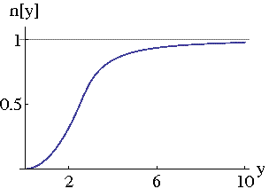
Figure 1: The density profile for an isolated vortex at the origin, as given by (22) for $y<2.7$ and (20) for $y>2.7$.

IV Linear Perturbation

Consider linear perturbations around a configuration of the 2D Bose gas with a vortex at the origin:

$$n=n_{q}(1+\delta),\zeta=-iq\varphi+\zeta_{1},$$ (23)

where $\delta=\delta(y,\varphi,s)$ and $\zeta_{1}=\zeta_{1}(y,\varphi,s)$ are functions of the radial and azimuthal coordinates $y$ and $\varphi$. Define the operator

$$\tilde{\nabla}_{y}^{2}=\frac{1}{yn_{q}}\frac{\partial}{\partial y}\left(yn_{q}\frac{\partial}{\partial y}\right)+\frac{1}{y^{2}}\frac{\partial^{2}}{\partial\varphi^{2}}.$$ (24)

Note that for $q=0$ (i.e., $n_{q}=1$), $\tilde{\nabla}_{y}^{2}=\nabla_{y}^{2}$. Putting the perturbation (23) in the action (15), it becomes

$$\mathcal{S}(q)\approx\mathcal{F}_{0}(q) + \frac{\hbar\mu\xi^{2}}{g}\int_{0}^{\mu\beta}ds\int d^{2}y\cdot n_{q}\delta\left(\frac{n_{q}}{2}-\frac{1}{2}\tilde{\nabla}_{y}^{2}\right)\delta$$

$$+ \frac{\hbar\mu\xi^{2}}{g}\int_{0}^{\mu\beta}ds\int d^{2}y\cdot\zeta_{1}\left(2n_{q}\tilde{\nabla}_{y}^{2}\right)\zeta_{1}$$

$$+ \frac{\hbar\mu\xi^{2}}{g}\int_{0}^{\mu\beta}ds\int d^{2}y\cdot n_{q}\zeta_{1}\left(\frac{\partial}{\partial s}-\frac{4iq}{y^{2}}\frac{\partial}{\partial\varphi}\right)\delta,$$

where

$$\mathcal{F}_{0}(q) = \frac{\hbar\mu\xi^{2}}{g}\int_{0}^{\mu\beta}ds\int d^{2}y\cdot\left[\frac{2n_{q}q^{2}}{y^{2}}-n_{q}+\frac{n_{q}^{2}}{2}+\frac{1}{2n_{q}}\left(\frac{dn_{q}}{dy}\right)^{2}\right]$$ (26)

$$= -\frac{\pi\hbar\xi^{2}\mu^{2}\beta}{g}\int dy\cdot yn_{q}^{2},$$

which is the equilibrium free energy, with the second equality owing to (18). Then the equations of motion are given by

$$\frac{\partial\zeta_{1}}{\partial s}=n_{q}\delta+\frac{4iq}{y^{2}}\frac{\partial\zeta_{1}}{\partial\varphi}-\tilde{\nabla}_{y}^{2}\delta,$$ (27)

$$\frac{\partial\delta}{\partial s}=\frac{4iq}{y^{2}}\frac{\partial\delta}{\partial\varphi}-4\tilde{\nabla}_{y}^{2}\zeta_{1}.$$ (28)

The Fourier transform of the fluctuations can be defined as

$$\delta(y,\varphi,s)=\sum_{j=-\infty}^{\infty}\delta_{j}(y,s)e^{ij\varphi},$$ (29)

$$\zeta_{1}(y,\varphi,s)=\sum_{j=-\infty}^{\infty}\zeta_{1j}(y,s)e^{ij\varphi}.$$ (30)

If $\delta$ and $\zeta_{1}$ are real, then

$$\delta_{j}^{*}=\delta_{-j},\zeta_{1j}^{*}=\zeta_{1-j}.$$ (31)

The representation (30) assumes that

$$\oint d\mathbf{l}\cdot\nabla\zeta_{1}=0,$$ (32)

which means the fluctuation does not change the total vorticity. The counterpart of $-\tilde{\nabla}_{y}^{2}$ in the Fourier representation is

$$L_{jq}=-\frac{1}{yn_{q}}\frac{\partial}{\partial y}\left(yn_{q}\frac{\partial}{\partial y}\right)+\frac{j^{2}}{y^{2}}.$$ (33)

The action (IV) becomes

$$\mathcal{S}(q)\approx\mathcal{F}_{0}(q) + \frac{\hbar\mu\xi^{2}}{g}\int_{0}^{\mu\beta}ds\int dy\cdot yn_{q}\sum_{j=-\infty}^{\infty}\delta_{-j}\left(\frac{n_{q}}{2}+\frac{1}{2}L_{jq}\right)\delta_{j}$$

$$+ \frac{\hbar\mu\xi^{2}}{g}\int_{0}^{\mu\beta}ds\int dy\cdot yn_{q}\sum_{j=-\infty}^{\infty}\zeta_{1-j}\left(-2L_{jq}\right)\zeta_{1j}$$

$$+ \frac{\hbar\mu\xi^{2}}{g}\int_{0}^{\mu\beta}ds\int dy\cdot yn_{q}\sum_{j=-\infty}^{\infty}\zeta_{1-j}\left(\frac{\partial}{\partial s}+\frac{4qj}{y^{2}}\right)\delta_{j}.$$

This action can be further simplified. Define

$$\hat{L}_{jq}=\left[-\frac{1}{y}\frac{\partial}{\partial y}\left(y\frac{\partial}{\partial y}\right)+\frac{j^{2}}{y^{2}}\right]+\left(\frac{q^{2}}{y^{2}}-\frac{1-n_{q}}{2}\right).$$ (35)

Suppose $F$ and $f$ are related by $F=\frac{f}{\sqrt{n_{q}}}$, then $L_{jq}$ and $\hat{L}_{jq}$ are related by

$$L_{jq}F=\frac{1}{\sqrt{n_{q}}}\hat{L}_{jq}f.$$ (36)

Define the covariant differential operator,

$$D_{s,jq}=\frac{\partial}{\partial s}-\frac{4qj}{y^{2}},$$ (37)

which can be seen as the time-derivative in a frame corotating with the vortex. With the transformation of the fluctuations,

$$\delta_{j}=\frac{\hat{\delta}_{j}}{\sqrt{n_{q}}},\zeta_{1j}=\frac{\hat{\zeta}_{1j}}{\sqrt{n_{q}}},$$ (38)

the action (IV) is then rewritten as

$$\mathcal{S}(q) \approx \mathcal{F}_{0}(q)+\frac{\hbar\mu\xi^{2}}{g}\int_{0}^{\mu\beta}ds\int dy\cdot y\sum_{j=-\infty}^{\infty}$$

$$\left[\hat{\delta}_{-j}\frac{n_{q}+\hat{L}_{jq}}{2}\hat{\delta}_{j}-\hat{\zeta}_{1-j}(2\hat{L}_{jq})\hat{\zeta}_{1j}+\hat{\zeta}_{1-j}D_{s,jq}\hat{\delta}_{j}\right].$$

From (27) and (28), or from the action (IV), the equations of motion in terms of the new operators are

$$(n_{q}+\hat{L}_{jq})\hat{\delta}_{j}=D_{s,-jq}\hat{\zeta}_{1j},$$ (40)

$$4\hat{L}_{jq}\hat{\zeta}_{1j}=D_{s,jq}\hat{\delta}_{j}.$$ (41)

V Lifetime of the Condensate

Consider a Bose gas confined to a region of size $L$. We define as our system a part of the Bose gas with linear size $l$ smaller than $L$ but greater than the healing length $\xi$, i.e., $L\gg l\gg\xi$. The Bose gas within this system is interacting with other atoms outside, which act as a reservoir of energy, particle number and angular momentum. Therefore the total vorticity $q$ of our system is not conserved. The equilibrium state is described by the partition function Altland and Simons (2006)

$$\mathcal{Z}=\sum_{q=-\infty}^{\infty}\int d\delta d\zeta_{1}\int D[\delta]D[\zeta_{1}]\exp\left(-\frac{\mathcal{S}(q)}{\hbar}\right),$$ (42)

where the periodic boundary conditions Negele and Orland (1998) $\delta=\delta(0)=\delta(\mu\beta)$ and $\zeta_{1}=\zeta_{1}(0)=\zeta_{1}(\mu\beta)$ have been incorporated in the evaluation of the path integral.

Setting an upper cutoff at $y=\Lambda$, the Euclidean action (essentially the free energy divided by $k_{B}T$) of the system with no vortex is obtained by putting $n_{0}=1$ in (26)

$$\mathcal{F}(0)=-\frac{\pi\hbar\xi^{2}\mu^{2}\beta}{g}\int_{0}^{\Lambda}dy\cdot y=-\frac{\pi\hbar\xi^{2}\mu^{2}\beta}{g}\frac{\Lambda^{2}}{2},$$ (43)

and that with one vortex of vorticity $q$ is obtained after putting the asympotic expressions (20) and (22) in (26),

$$\mathcal{F}(q) = -\frac{\pi\hbar\xi^{2}\mu^{2}\beta}{g}\int_{0}^{\Lambda}dy\cdot yn_{q}^{2}$$ (44)

$$\approx -\frac{\pi\hbar\xi^{2}\mu^{2}\beta}{g}\left(\frac{\Lambda^{2}}{2}-4q^{2}\ln\Lambda\right),$$

as at small $y$ the integral vanishes in both cases. As a result, adding a vortex means adding an amount of the Euclidean action

$$\Delta\mathcal{F}(q)=\frac{4\pi\hbar\xi^{2}\mu^{2}\beta q^{2}}{g}\ln\Lambda.$$ (45)

Suppose $K_{0}$ is the fluctuation factor calculated from the path integral in (42) around the $q=0$ configuration, and $K_{0}K_{1}$ is that around the $q=1$ configuration. If ${\kappa_{jq}^{\alpha}}^{2}$’s are the eigenvalues of $\hat{L}_{jq}$, then the partition function of the $q=0$ case is given by Feynman (1972)

$$K_{0}=\prod_{\alpha,j}\frac{1}{2\sinh\frac{\sqrt{4{\kappa_{j0}^{\alpha}}^{2}(1+{\kappa_{j0}^{\alpha}}^{2})}\mu\beta}{2}}.$$ (46)

For $q=1$, the translation invariance of the vortices gives rise to the existence of the zero modes Rajaraman (1987). We know that we can generate solutions with $\omega=0$ by simply moving the vortex around. Since the vortex is already rotation invariant, it is enough to consider a vortex centered at $x=R$. The displaced vortex solution is given by $n=n_{q}\left(y^{\prime}\right)$, $\zeta=q\varphi^{\prime}$, where

$$y^{\prime}=\sqrt{y^{2}+R^{2}-2yR\cos\varphi},\\ y^{\prime}\sin\varphi^{\prime}=y\sin\varphi,$$ (47)

For small $R$ we have

$$y^{\prime}=y-R\cos\varphi,\\ \varphi^{\prime}=\varphi+\frac{R}{y}\sin\varphi,$$ (48)

and the deviation from the centered vortex is

$$\bar{\zeta}_{1}=\frac{qR}{y}\sin\varphi,\\ \bar{\delta}=-R\frac{1}{n_{q}}\frac{dn_{q}}{dy}\cos\varphi$$ (49)

Then the zero-mode action $S_{0}$ is given by

$$S_{0}\approx S[\bar{\delta},\bar{\zeta}_{1}].$$ (50)

If $\hat{\Lambda}_{0}$ is the operator for $q=0$ and $\hat{\Lambda}_{1}$ for $q=1$, then the fluctuation factor is given by

$$K_{1}=\left[\frac{\det\hat{\Lambda}_{0}}{\det\hat{\Lambda}_{1}}\right]^{\frac{1}{2}}=\sqrt{\frac{S_{0}}{2\pi\hbar}}\left[\frac{\det\hat{\Lambda}_{0}}{\det^{\prime}\hat{\Lambda}_{1}}\right]^{\frac{1}{2}},$$ (51)

where the second equality is due to the existence of a zero mode because of the translational invariance of the vortices Coleman (1985); Affleck and De Luccia (1979), and $\det^{\prime}$ is the determinant excluding the zero mode. The ratio of the determinants is given by the Gelfand-Yaglom theorem Gelfand and Yaglom (1960); Dunne (2008).

Now consider the situation where more than one vortex is formed. In the dilute gas approximation the vortices are assumed to be far apart so adding $n$ vortices of vorticity $q=1$ increases the Euclidean action by $n\Delta\mathcal{F}(1)$ C. G. Callan and Coleman (1977); Coleman (1985). Form a statistical ensemble of different numbers of vortices $n$, the partition function is given by

$$\mathcal{Z} \approx e^{-\frac{\mathcal{F}_{0}(0)}{\hbar}}\sum_{n=0}^{\infty}\int d^{2}y_{1}\int d^{2}y_{2}\ldots\int d^{2}y_{n}\cdot\frac{1}{n!}K_{0}(K_{1})^{n}e^{-n\frac{\Delta\mathcal{F}}{\hbar}}$$ (52)

$$= K_{0}\exp\left(-\frac{\mathcal{F}_{0}(0)}{\hbar}+\Lambda^{2}K_{1}e^{-\frac{\Delta\mathcal{F}}{\hbar}}\right),$$

where the integrations over the space have an upper cutoff $\Lambda^{2}$, and the factor $\frac{1}{n!}$ is due to the indistinguishability of the vortices. The decay probability per unit time of the configuration from $q=0$ to $1$ is C. G. Callan and Coleman (1977)

$$\Gamma=-\frac{2}{\hbar}\mathrm{Im}\mathcal{F}=\frac{1}{\hbar\beta}\mathrm{Im}(K_{1})e^{-\frac{\Delta\mathcal{F}(1)}{\hbar}+2\ln\Lambda}.$$ (53)

From the expression of the decay probability, the BKT transition temperature can be read off from the exponential factor since the formation occurs at a reasonable rate as $e^{-\frac{\Delta\mathcal{F}}{\hbar}+2\ln\Lambda}\sim 1$. It is given by

$$T_{BKT}\approx\frac{2\pi\xi^{2}\mu^{2}}{gk_{B}}=\frac{\pi\hbar^{2}\rho_{0}}{2mk_{B}},$$ (54)

where the definition of healing length $\xi$ in (9) is used and $\rho_{0}=\mu/g$ Ginzburg and Pitaevskii (1958) is the number density of the lowest macroscopically occupied state of the homogeneous configuration $n_{0}=1$. This agrees with the known results in the original BKT theory Kosterlitz and Thouless (1973). The correction due to non-homogeneneous configuration in the transition temperature is given in Ref. Holzmann et al. (2008); Holzmann and Krauth (2008).

Because $K_{1}$ is given as the square root of the ratio of the determinants of two differential operators, we expect it is of order $1$. Then by dimensional analysis, $\Gamma\sim\frac{1}{\hbar\beta}\sim 13.1$ ms^-1. The average time of vortex formation is then of the order of $0.08$ ms. The numerical estimation of the vortex nucleation rate around the transition temperature with the estimated numerical parameters listed in Sec. II is plotted as shown in Fig. 2. The vortex formation is very slow below the transition temperature but it increases drastically when the temperature increases past the critical point.

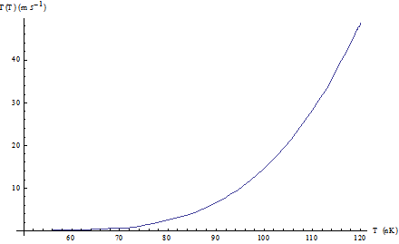
Figure 2: The rate of vortex nucleation around the BKT transition temperature.

VI Computing the imaginary part of the free energy

The expression for the decay rate in (53) shows that under the dilute gas approximation the stability of the canonical equilibrium hinges on whether the path integral over fluctuations around a one-vortex configuration is complex.

Recall that the action for a linearized fluctuation is given by (IV), where the $\hat{L}_{jq}$ operators are defined in (35). We perform the Gaussian path integration over $\zeta_{1}$ to obtain

$$\mathcal{S}(q) \approx \mathcal{F}_{0}(q)+\frac{\hbar\mu\xi^{2}}{g}\int_{0}^{\mu\beta}ds\int dy\cdot y\sum_{j=-\infty}^{\infty}$$ (55)

$$\left[\hat{\delta}_{-j}\frac{n_{q}+\hat{L}_{jq}}{2}\hat{\delta}_{j}+\frac{1}{8}(\hat{L}_{jq}^{-1}D_{s,-jq}\hat{\delta}_{-j})(D_{s,jq}\hat{\delta}_{j})\right].$$

If the $\hat{L}_{jq}$ operators are positive definite, it is clear that the path of steepest descent away from the stationary point corresponds to real $\delta_{j}$, and the path integral is real.

This is indeed so when we are considering fluctuations around a homogeneous configuration, namely $q=0$, $n_{q}=1$. In this case, the eigenvectors of $\hat{L}_{j0}$ are Bessel functions of order $j$. The requirement that the Euclidean action must be finite means that we only need to consider eigenfunctions which do not diverge at infinity and are regular at the origin. The only Bessel functions satisfying these conditions are of the form $J_{j}\left[\kappa y\right]$ corresponding to a positive eigenvalue $\kappa^{2}$. Thus we conclude that the no-vortex state is stable at zero temperature, when the no-vortex configuration is the only finite action extremal point in the partition function.

Let us see if this argument carries over for nonzero $q$. For simplicity, we set $q=1$ (however, we shall leave $q$ explicit). We seek finite action solutions to the equation

$$\hat{L}_{jq}F^{\kappa}_{jq}\left(y\right)=-\kappa^{2}F^{\kappa}_{jq}\left(y\right),$$ (56)

with real $\kappa$. The further change of variables

$$F^{\kappa}_{jq}\left(y\right)=\frac{f^{\kappa}_{jq}\left(y\right)}{\sqrt{y}},$$ (57)

reduces the left hand side to a Schrodinger operator

$$\left[-\frac{d^{2}}{dy^{2}}+V_{jq}\left(y\right)\right]f^{\kappa}_{jq}\left(y\right)=-\kappa^{2}f^{\kappa}_{jq}\left(y\right),$$ (58)

where

$$V_{jq}\left(y\right)=\frac{j^{2}+q^{2}-\frac{1}{4}}{y^{2}}-\frac{1}{2}\left(1-n_{q}\left(y\right)\right).$$ (59)

Therefore the question of whether the Euclidean action for linearized fluctuations around an isolated vortex is positive definite becomes whether a one-dimensional particle of mass $1/2$ in the potential (59) admits a negative energy state. Now, the potential happens to be everywhere positive for all $j>0$, so we may discard this possibility outright unless $j=0$ (see Fig. 3)

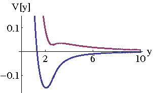
Figure 3: The effective potential Eq. (59) for $j=1$ (upper curve) and $j=0$ (lower curve). We have used the profile in Fig 1 to compute $n_{q}$. We see that for $j=1$ there can be no negative energy state, even more so for larger values of $j$. For $j=0$, on the other hand, the potential is negative for large enough values of $y$. The existence of a negative energy states is shown by Bohr-Sommerfeld condition as in (60).

In the $j=0$ case there is a well defined potential well, and we must investigate whether it is deep enough to support a bound state. One possibility is to check the Bohr-Sommerfeld condition, namely, whether there is a value of $\kappa$ such that

$$\int_{y_{-}}^{y_{+}}dy\>\sqrt{-\kappa^{2}-V_{01}\left(y\right)}=\frac{\pi}{2},$$ (60)

where $y_{\pm}$ are the classical turning points, namely the roots of $\kappa^{2}+V_{01}\left(y\right)=0$. The answer turns out to be yes though just barely. Under the approximation given in Fig. 1 for the density profile, the Bohr-Sommerfeld condition is satisfied for $\kappa=0.024$. The turning points are located at $y_{-}=1.32$ and $y_{+}=21.2$. Bohr-Sommerfeld quantization would also predict bound excited states; however, these states fall beneath the accuracy of our approximations, and they may be considered artifacts. For example, according to Bohr-Sommerfeld quantization the first excited state appears at $\kappa=4\times 10^{-5}$, with the outer turning point at $y=12,500$. This is beyond the intended size of the original homogeneous patch, because from the numerical estimation in Sec. II, the size of the patch in the dimensionless unit is $\sqrt{\frac{R_{\bot}}{\xi}}\sim 40$, which is far less than $12,500$.

Observe that not only have we shown that the Euclidean action for axially symmetric perturbations of the isolated vortex is not positive definite, but we have also characterized the eigenvector corresponding to the direction in configuration space where it becomes negative. Since $n_{q}$ does not commute with $\hat{L}_{01}$, this eigenvector does not correspond to an actual solution of the linearized fluctuations. However, its existence is enough to show that the free energy acquires an imaginary part.

VII Summary and Discussions

In this work we have calculated the rate of decay of an effectively homogeneous 2D Bose gas (described by $V(\mathbf{x})=0$), in the form of $Ae^{-\frac{B}{T}}$, which complies with the well-known Arrhenius law. The prefactor $A$ is proportional to the imaginary part of the fluctuation factor of the free energy of a one-vortex configuration in the path integral. It is known that this imaginary part is due to the negative eigenvalue of the fluctuation operator belonging to the eigenvector that defines the direction the fluctuation spontaneously grows along (in real time). The qualitative features are like those in the decay of a metastable state due to classical fluctuations Langer (1969) and barrier penetration due to quantum fluctuations around the instanton solution of the Euclidean action C. G. Callan and Coleman (1977). We find that the imaginary part comes from the axially-symmetric modes for nonzero vorticity configurations. As a result, we conclude that while at $T=0$, the gas without any vortex is stable, the canonical ensemble of different numbers of vortices of the gas is unstable at any finite temperature.

Using the fact that at the BKT transition $Ae^{-\frac{B}{T}}\sim 1$ we derived the BKT transition temperature ${T_{BKT}}$ in terms of the number density of the homogeneous phase given in (54). This expression derived via thermal field theory provides a more quantitative alternative to that originally derived from thermodynamics considerations of the competition between the energy and the entropy of a vortex Kosterlitz and Thouless (1973). It is known that isolated free vortices are formed in the normal phase above the BKT temperature. Hence the decay rate calculated here is also the rate of vortex formation. Our calculations show how it increases with temperature. The probability of the creation of vortex pairs in a trapped gas increases with temperature as well, as indicated by simulation studies with the PGPE Simula and Blakie (2006).”

In the experiments, measurements on the gas are made some time after the confining potential is abruptly turned off. In Dalibard group’s experiment there are more isolated free vortices (measured by the dislocation of interference pattern of two planes of gas) at higher temperature after 20 ms time of flight (TOF) Hadzibabic et al. (2007). Our results are consistent with this finding in that the rate of isolated vortex formation increases with temperature. In Phillips group’s experiment Cladé et al. (2009), they observed different characteristics on the density profile below and above the BKT temperature after 10 ms TOF, which is at a rate slower than the rate of the formation of isolated vortices. However, since we have assumed a homogeneous, time-independent configuration as starting point, this should factor in the comparison of our results with experiments. Further studies to bridge these gaps are desirable.

References

- Mermin and Wagner (1966) N. D. Mermin and H. Wagner, Phys. Rev. Lett. 17, 1133 (1966).
- Hohenberg (1967) P. C. Hohenberg, Phys. Rev. 158, 383 (1967).
- Coleman (1973) S. Coleman, Comm. Math. Phys. 31, 259 (1973).
- Berezinskii (1971) V. L. Berezinskii, Sov. Phys. JETP 32, 493 (1971).
- Kosterlitz and Thouless (1973) J. M. Kosterlitz and D. J. Thouless, J. Phys. C: Solid State Phys. 6, 1181 (1973).
- Khawaja et al. (2002) U. A. Khawaja, J. O. Andersen, N. P. Proukakis, and H. T. C. Stoof, Phys. Rev. A 66, 013615 (2002), eprint cond-mat/0202085.
- How and LeClair (2010) P.-T. How and A. LeClair, Nucl. Phys. B824, 415 (2010), eprint arXiv:0906.0333.
- Gräter and Wetterich (1995) M. Gräter and C. Wetterich, Phys. Rev. Lett. 75, 378 (1995), eprint hep-ph/9409459.
- Gersdorff and Wetterich (2001) G. V. Gersdorff and C. Wetterich, Phys. Rev. B 64, 054513 (2001), eprint hep-th/0008114.
- Floerchinger and Wetterich (2009) S. Floerchinger and C. Wetterich, Phys. Rev. A 79, 013601 (2009), eprint arXiv:0805.2571.
- Popov (1973) V. N. Popov, Sov. Phys. JETP 37, 341 (1973).
- Popov (1987) V. N. Popov, Functional Integrals and Collective Excitations (Cambridge University Press, Cambridge, England, 1987), chap. 8.
- Chu and Williams (2000) H.-C. Chu and G. A. Williams, Phys. Rev. Lett. 86, 2585 (2000).
- Arovas and Auerbach (2008) D. P. Arovas and A. Auerbach, Phys. Rev. B 78, 094508 (2008).
- Lindner et al. (2008) N. H. Lindner, A. Auerbach, and D. P. Arovas, Phys. Rev. Lett. 102, 070403 (2008), eprint arXiv:0810.2604.
- Wang et al. (2010) C.-C. J. Wang, R. A. Duine, and A. H. MacDonald, Phys. Rev. A 81, 013609 (2010), eprint arXiv:0910.0205.
- Gross (1963) E. P. Gross, J. Math. Phys. 4, 195 (1963).
- Ginzburg and Pitaevskii (1958) V. L. Ginzburg and L. P. Pitaevskii, Sov. Phys. JETP 34, 858 (1958).
- Pu et al. (1999) H. Pu, C. K. Law, J. H. Eberly, and N. P. Bigelow, Phys. Rev. A 59, 1533 (1999), eprint cond-mat/9807362.
- Prokof’ev et al. (2001) N. Prokof’ev, O. Ruebenacker, and B. Svistunov, Phys. Rev. Lett. 87, 270402 (2001).
- Prokof’ev and Svistunov (2002) N. Prokof’ev and B. Svistunov, Phys. Rev. A 66, 043608 (2002).
- Davis et al. (2002) M. J. Davis, S. A. Morgan, and K. Burnett, Phys. Rev. A 66, 053618 (2002).
- Hutchinson and Blakie (2006) D. A. W. Hutchinson and P. B. Blakie, Int. J. Mod. Phys, B 20, 5224 (2006), eprint cond-mat/0602614.
- Simula and Blakie (2006) T. P. Simula and P. B. Blakie, Phys. Rev. Lett. 96, 020404 (2006), eprint cond-mat/0510097.
- Shumayer and Hutchinsin (2007) D. Shumayer and D. A. W. Hutchinsin, Phys. Rev. A 75, 015601 (2007).
- Simula et al. (2008) T. P. Simula, M. J. Davis, and P. B. Blakie, Phys. Rev. A 77, 023618 (2008), eprint arXiv:0711.1423.
- Holzmann et al. (2008) M. Holzmann, M. Chevallier, and W. Krauth, Europhys. Lett. 82, 30001 (2008).
- Bisset et al. (2009a) R. N. Bisset, D. Baillie, and P. B. Blakie, Phys. Rev. A 79, 013602 (2009a).
- Bisset et al. (2009b) R. N. Bisset, M. J. Davis, T. P. Simula, and P. B. Blakie, Phys. Rev. A 79, 033626 (2009b), eprint arXiv:0804.0286.
- Bisset and Blakie (2009a) R. N. Bisset and P. B. Blakie, Phys. Rev. A 80, 045603 (2009a).
- Bisset and Blakie (2009b) R. N. Bisset and P. B. Blakie, Phys. Rev. A 80, 035602 (2009b).
- Hadzibabic et al. (2007) Z. Hadzibabic, P. Krüger, M. Cheneau, B. Battelier, and J. Dalibard, Nature 441, 1118 (2007), eprint cond-mat/0605291.
- Krüger et al. (2007) P. Krüger, Z. Hadzibabic, and J. Dalibard, Phys. Rev. Lett. 99, 040402 (2007), eprint cond-mat/0703200.
- Cladé et al. (2009) P. Cladé, C. Ryu, A. Ramanathan, K. Helmerson, and W. D. Phillips, Phys. Rev. Lett. 102, 170401 (2009), eprint arXiv:0805.3519.
- Esteban Calzetta and Bei-Lok Hu (2008) Esteban Calzetta and Bei-Lok Hu, Nonequilibrium Quantum Field Theory (Cambridge University Press, Cambridge, England, 2008), chap. 13.3.
- Rubakov (2002) V. Rubakov, Classical theory of gauge fields (Princeton University Press, Princeton, NJ, 2002).
- Langer (1968) J. S. Langer, Phys. Rev. Lett. 21, 973 (1968).
- Langer (1969) J. S. Langer, Ann. Phys. 54, 258 (1969).
- Coleman (1977) S. Coleman, Phys. Rev. D 15, 2929 (1977).
- C. G. Callan and Coleman (1977) J. C. G. Callan and S. Coleman, Phys. Rev. D 16, 1762 (1977).
- Coleman (1985) S. Coleman, Aspects of Symmetry (Cambridge University Press, Cambridge, England, 1985), chap. 7.
- Affleck and De Luccia (1979) I. K. Affleck and F. De Luccia, Phys. Rev. D 20, 3168 (1979).
- Affleck (1981) I. Affleck, Phys. Rev. Lett. 46, 388 (1981).
- Haldane (1981) F. D. M. Haldane, Phys. Rev. Lett. 47, 1840 (1981).
- Calzetta et al. (2006) E. Calzetta, B. L. Hu, and A. M. Rey, Phys. Rev. A 73, 023610 (2006).
- Hadzibabic and Dalibard (2009) Z. Hadzibabic and J. Dalibard (2009), eprint arXiv:0912.1490.
- Lifshitz and Pitaevskii (1990) L. M. Lifshitz and L. P. Pitaevskii, Statistical Physics, Part 2 (Pergamon Press, Oxford, 1990), vol. 9 of Course of Theoretical Physics, chap. 30.
- Barnett et al. (2010) R. Barnett, E. Chen, and G. Refael, New J. Phys. 13, 043004 (2010), eprint arXiv:0909.4072.
- Altland and Simons (2006) A. Altland and B. Simons, Condensed Matter Field Theory (Cambridge, Cambridge, England, 2006), chap. 9.
- Negele and Orland (1998) J. W. Negele and H. Orland, Quantum Many-Particle Systems (Perseus, New York, NY, 1998), chap. 2.2.
- Feynman (1972) R. P. Feynman, Statistical Mechanics (Addison Wesley, Reading, Massachusetts, 1972), chap. 3.
- Rajaraman (1987) R. Rajaraman, Solitons and Instantons (Elsevier, New York, NY, 1987), chap. 10.
- Gelfand and Yaglom (1960) I. M. Gelfand and A. M. Yaglom, J. Math. Phys. 1, 48 (1960).
- Dunne (2008) G. V. Dunne, J. Phys. A: Math. Theor. 41, 304006 (2008), eprint arXiv:0711.1178.
- Holzmann and Krauth (2008) M. Holzmann and W. Krauth, Phys. Rev. Lett. 100, 190402 (2008), eprint arXiv:0710.5060.