A Wide-Field Survey of the Orion Nebula Cluster in the Near-Infrared

Abstract

We present J, H and K_S photometry of the Orion Nebula Cluster obtained at the CTIO/Blanco 4 m telescope in Cerro Tololo with the ISPI imager. From the observations we have assembled a catalog of about $\sim 7800$ sources distributed over an area of approximately $30\arcmin\times 40\arcmin$, the largest of any survey deeper than 2MASS in this region. The catalog provides absolute coordinates accurate to about 0.15 arcseconds and $3\sigma$ photometry in the 2MASS system down to $\hbox{\sl J}\simeq 19.5$ mag, $\hbox{\sl H}\simeq 18.0$ mag, $\hbox{\sl K{${}_{S}$}}\simeq 18.5$ mag, enough to detect planetary size objects 1 Myr old under $A_{V}\simeq 10$ mag of extinction at the distance of the Orion Nebula. We present a preliminary analysis of the catalog, done comparing the (J-H,H-K_S) color-color diagram, the (H,J-H) and (K_S,H-K_S) color-magnitude diagrams and the JHK_S luminosity functions of three regions at increasing projected distance from the Trapezium. Sources in the inner region typically show IR colors compatible with reddened T Tauri stars, whereas the outer fields are dominated by field stars seen through an amount of extinction which decreases with the distance from the center. The color-magnitude diagrams make it possible to clearly distinguish between the main ONC population, spread across the full field, and background sources. The luminosity functions of the inner region, corrected for completeness, remain relatively flat in the sub-stellar regime regardless of the strategy adopted to remove background contamination.

1 Introduction

The Orion Nebula hosts the richest cluster of  young ($\tau\simeq 1$ Myr) Pre-Main-Sequence (PMS) stars within 1 kpc of the Sun and therefore represents an ideal laboratory to understand the process of star formation (see Muench et al., 2008; O’Dell, 2008, for recent reviews). The cluster, both rich ($n\approx 2000$ members) and dense (about $2\times 10^{4}$ sources per cubic parsec at its center), is dominated by a small number of massive OB stars mostly clustered in the Trapezium multiplet ($\theta^{1}$ Ori). Their UV emission has created a blister HII   region (Orion Nebula, M 42, NGC 1976) whose ionization front is still carving the underlying Orion Molecular Cloud (OMC-1, O’Dell, 2008; O’Dell et al., 2009). About half of the young cluster members, surrounded by their original circumstellar disks, have been already exposed to the hard-UV radiation of the Trapezium stars, whereas the other half remain enshrouded within the OMC-1, together with newer active sites of star formation.

Visible and near-IR data, both in imaging and spectroscopy, are needed to characterize the main physical parameters of the cluster population (Hillenbrand, 1997). These observations, however, are hampered by the brightness and non-uniformity of the nebular background. To overcome these difficulties, we have exploited the unique combination of sensitivity and spatial resolution offered by the Hubble Space Telescope (HST) to obtain accurate photometry of the cluster, especially at substellar masses (HST Treasury program GO-10246). Our extensive HST survey has been complemented by ground-based observations, imaging the Orion Nebula from the U-band to the K_S-band at La Silla and Cerro Tololo (CTIO) observatories. The ground-based observations, carried out in parallel on the same nights (but at a different epoch than the HST observations), complement the deep HST data which saturate at relatively low brightness levels. Their simultaneity makes the derived stellar colors largely immune to the uncertainties associated with source variability.

The ground-based survey at visible wavelengths, performed with the Wide Field Camera (WFI) at the ESO/MPG 2.2 m telescope at La Silla, has been recently presented in Da Rio et al. (2009). In this paper we present the ground-based IR survey, performed at the CTIO/Blanco telescope with the ISPI imager. Its combination of sensitivity and field coverage (about $30\arcmin\times 40\arcmin$) ideally complements the previous surveys of this region. In particular, it reaches fainter magnitudes than the wide field survey ($30\arcmin\times 45\arcmin$) by Hillenbrand et al. (1998), while it covers a much larger area than the deep surveys done with Keck (HK_S-bands, $5\farcm 1\times 5\farcm 1$, Hillenbrand & Carpenter, 2000), HST-NICMOS (JH-bands, $2\farcm 3\times 2\farcm 3$, Luhman et al. 2000), UKIRT (IJH-bands, 36 arcmin², Lucas & Roche 2000), NTT (JHK_S, $5\arcmin\times 5\arcmin$, Muench et al. 2002) and Gemini (JHK_S-bands, 26 arcmin², Lucas et al. 2005). All these deep surveys concentrate on a field centered around the Trapezium stars, or in its immediate surroundings in the case of Lucas & Roche (2000).

In Section 2 we discuss the observing strategy, while in Section 3 we describe the data reduction and photometric calibration. In Section 4 we present our completeness analysis. The resulting source catalog is presented in Section 5, whereas in Section 6 we discuss the color-color and color-magnitude diagrams and the luminosity function derived from our J, H, and K_S-band photometry.

2 ISPI observations

The Infrared Side Port Imager (ISPI) is the facility infrared camera at the CTIO Blanco 4 m telescope. ISPI uses a 2k $\times$ 2k HgCdTe HAWAII-2 array, with reimaging optics providing a scale of 0.3 arcsec/pixel corresponding to a 10.25 $\times$ 10.25 arcmin field of view. Our target area, about $30\arcmin\times 40\arcmin$, covers the field imaged with the HST.

The observations were performed on the nights of 1 and 2 January 2005 (indicated hereafter as Night A and Night B respectively) in the J, H and K_S filters using the Double Correlated Sampling readout mode. The main filter parameters are listed in Table 1. The seeing was $\simeq 0\farcs 7$ in most of the K_S-band images and occasionally worse on night B.

The survey area was divided into eleven fields (Figure 1). The central position of each field, together with the airmass of the observations, is listed in Table 2. Each field was observed with an ABBA pattern. After pointing the telescope to the center of a field (A position) a 5 point dithering pattern was executed offsetting the telescope approximately by $\pm 30\arcsec$ along the field diagonals. This first group of 5 dithered exposures was followed by a second group of sky frames (B position)  taken on a nearby field free, or nearly free, of diffuse nebular emission to extend the field coverage and monitor the flat-field response close in time to our observations. The sky-source sequence was then repeated back, completing the ABBA cycle. This provides a total of 10 frames of 30 s exposure for the common part of each field, totalling 300 s integration. Due to the high background, we split the K_S-band 30 s exposures in two consecutive 15 s exposures, maintaining the background well within the linear regime.

Each dithering sequence was repeated with a 3 s integration time. These short frames were coadded into another image of 30 s total integration time, which we used to extract the photometry of sources saturated in the longer exposures. Due to an error in our observing procedure, the J-band observations of field 3 were obtained only with 3 s exposures.

For absolute calibration we observed at various airmass the faint IR standard stars 9108, 9118 and 9133 of Persson et al. (1998). Unfortunately, on both nights the atmospheric transmission at IR wavelengths turned out to be unstable due to variations in the water vapor opacity, and we eventually derived the zero point calibration of our images through comparison with the extensive set of 2MASS data across our wide field area, as described in Section 3.2.

3 Analysis

The first step in the data reduction was the correction for the intrinsic non-linearity of the detector, which we performed by applying the correction curve kindly provided by N. Van der Bliek. We flat-fielded each image using dome flats and correct for residual color terms at low-spatial frequency using delta-flats derived from median averaged sky images. The dome flats were also used to flag bad pixels. The sky frames, properly filtered to remove spurious sources arising from the latent images of bright stars on the infrared detectors, were combined and subtracted from the science images.

Since ISPI exhibits significant field distortion, each science image had to be geometrically corrected before being combined in a dithering group. This required a first pass of aperture photometry with DAOPHOT, in order to extract a source catalog with well measured centroids and photometry (to disentangle the case of multiple candidates in the search radius). These sources were then cross-identified with the 2MASS catalog for astrometric reference, building an image distortion map relating their position on the original images to the actual position provided by 2MASS. Due to the non-uniform distribution of sources, clustered at the center of the nebula, the accuracy of the distortion correction map varies across each field. Therefore, we combined the distortion maps relative to all images taken on the same night to derive, for each filter, a master distortion map. Each individual image was then warped using a 4th-order polynomial fit with coefficients derived from the corresponding distortion map. Images belonging to the same dithered groups were then combined per integer pixels into single $2500\times 2500$ images. The DAOPHOT source extraction was then repeated on these geometrically corrected images to produce a new source catalog from which we derived the final astrometric solution of each image by minimizing the residual shift and rotation with respect to the 2MASS positions. The average scatter between our coordinates and the corresponding 2MASS coordinates turns out to be about 0.15 arcsec, i.e., half of a ISPI pixel. The same procedure has been adopted on the 3 s images.

In conclusion, for each field the final data consist of one combined image in each of the 3 filters (J, H, K_S) and exposure times (300 s and 30 s), with the exception of fields 4, 5, and 6, which have double this number of images, and field 3, which was not observed with deep J  images.

3.1 Instrumental magnitudes

The extraction of source photometry was performed on the final combined images, for both short and long exposure times. The Daophot FIND IDL procedure was used to extract an initial list of candidate sources, with rather loose detection thresholds and criteria to include the largest possible number of candidates. This initial list, counting more than 60,000 candidates, has been visually inspected on the original images to clean up artifacts and to preliminarily classify real sources as either point-like or extended. The list was then reduced to 7563 sources, divided between 6305 point-like and 933 diffuse.

For all sources we first derived an aperture magnitude by integrating the flux over a 5 pixel (1.5 arcsec) radius circular aperture, taking sky annuli typically between 10 and 15 pixels (3.0-4.5 arcsec); for 1416 bright sources, saturated in the 30 s images, we used the photometry extracted from the 3 s images.

We then performed PSF photometry on all point-like sources. Due to the spatial variability of the PSF across the field of view of ISPI, present even after geometric correction, we divided each image in 9 parts (3$\times$3 squares) allowing for some overlap between adjacent sub-images. The samples of stars in each sub-image, still relatively rich, had a more homogeneous PSF  allowing us to reliably derive PSF magnitudes. We subtracted the PSFs and looked at the residual images searching for faint companion stars previously undetected. We found in this way 325 “hidden companions”. Finally, we performed a second pass of PSF photometry, first by removing from the list of stars used to derive the PSF those having a faint companion, and then deriving also the photometry of the newly detected faint companions.

3.2 Absolute calibration

As mentioned in Section 2, the IR photometric quality of our nights turned out to be unsatisfactory due to hygrometric variability. We therefore calibrated our ISPI instrumental magnitudes directly to the 2MASS photometric system. The 2MASS catalog provides absolute photometry in the J (1.25µm), H (1.65µm), and K_S (2.17µm) bands to a limiting magnitude of 15.8, 15.1, and 14.3, respectively, with signal-to-noise ratio greater than 10.

To estimate the color terms and zero points of each image, we first scaled the instrumental PSF magnitudes of point sources measured in the short 30 s images to the long 300 s images, chosen as the reference time because of their source richness. To minimize systematic effects due do atmospheric variations, we did not simply add the nominal $\Delta mag=2.5$ factor but compared the instrumental magnitudes of well measured stars to derive for each field and filter a mean magnitude offset $\overline{\Delta mag}$ between the short and long images. By homogenizing in this way the zero points of the short and long images, we add a small uncertainty to the photometric errors of the bright stars measured in the short exposures.

For each bandpass $\lambda$ we then evaluated the relations

$$mag_{\rm 2MASS}(\lambda)-mag_{\rm ISPI}(\lambda)=ZP_{\lambda}+\epsilon_{\lambda_{1},\lambda_{2}}\cdot c_{\rm ISPI}(\lambda_{1},\lambda_{2}),$$

where $mag_{\rm 2MASS}$ is the magnitudes in the 2MASS photometric system, $mag_{\rm ISPI}$ is the ISPI  instrumental magnitude, the intercept $ZP_{\lambda}$ is the zero point in a given bandpass, the slope $\epsilon_{\lambda_{1},\lambda_{2}}$ is a color coefficient between the wavelengths $\lambda_{1}$ and $\lambda_{2}$ and $c_{\rm ISPI}$ is the corresponding observed ISPI color. We found the strongest statistical correlation in the combination:

$$H_{\rm 2MASS}-H_{\rm ISPI}=ZP_{H}+\epsilon_{JK}\cdot(J-K)_{\rm ISPI}.$$

For each field, we derived the linear fit parameters $ZP_{H}$ and $\epsilon_{JK}$ using an iterative procedure to rejects spurious outliers and all sources with errors greater than $0.1^{m}$ in the 2MASS catalog and $0.05^{m}$ in our input catalog. As shown in Table 3, the color coefficient $\epsilon_{JK}$ varies slightly from field to field during each night, whereas the zeropoint $ZP_{\lambda}$ shows an increase towards the middle of the night (observation were scheduled with fields 4 and 10 transiting at the meridian, in the two nights).

For the J and K_S bands, we derived the zero-points and the color terms from a linear fit to the color relations

$$(J-H)_{\rm 2MASS}=ZP_{JH}+\epsilon_{JH}\cdot(J-H)_{\rm ISPI},$$

$$(H-K_{S})_{\rm 2MASS}=ZP_{HK}+\epsilon_{HK}\cdot(H-K_{S})_{\rm ISPI}.$$

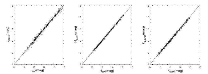
Figure 2: Comparison between 2MASS magnitudes and ISPI calibrated magnitudes.

This allowed us to derive magnitudes calibrated in the 2MASS system for all sources with ISPI $JHK$ instrumental photometry. In Figure 2 we show a comparison between the magnitudes reported in the 2MASS catalog and our calibrated magnitudes. The plots show the lack of systematic differences, besides the random errors that we attribute to photometric errors or stellar variability.

For sources lacking one or two magnitudes (typically either J or both J and H), we assumed a linear relation of this type

$$mag_{\rm 2MASS}(\lambda)=\alpha\times mag_{\rm ISPI}(\lambda)+\beta$$

deriving $\alpha$ and $\beta$, for each bandpass and field, from the sample of calibrated sources. The parameter $\alpha$ provides a magnitude-dependent correction to the zero point $\beta$, which is appropriate since fainter sources have, on average, redder colors. Using these coefficients we calibrated the magnitudes, with the relative uncertainties, of all remaining sources.

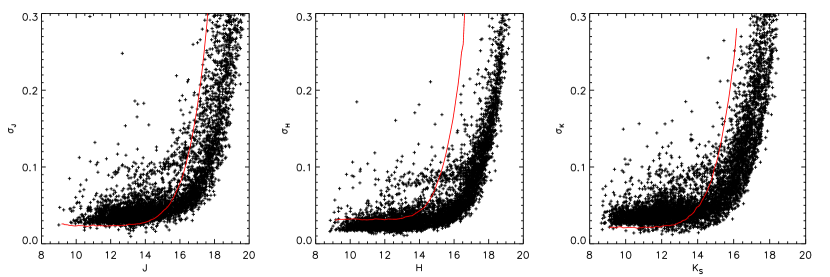
Figure 3: PSF photometric error as a function of magnitude for our point-like sources. The solid line indicates the locus of the average relation for the 2MASS sources falling in the ISPI field.

Figure 3 shows the photometric errors plotted as a function of magnitude for all point-like sources. The multiple threads in the distribution of the photometric errors are due either to the superposition of deep and short exposures (bright stars, measured in short 3 s exposures, turn out to have relatively larger errors) or to the sources measured, with higher photometric errors, in the crowded central part of the cluster. For comparison we also plot the average mag vs. Delta mag relation for the 2MASS  sources falling in our field.

4 Completeness

To determine the completeness of our photometric catalog, we used an artificial star experiment. For each field and filter, we averaged the 9 PSFs created for photometric extraction (Section 3.1) into a common reference PSF valid for the full image. We scaled the reference PSF in steps of 0.1 mag covering the entire magnitude range measured across each field and injected each scaled PSF  at a random position in the image, with the only caveat of leaving enough distance from the border to allow for a meaningful measure. We assumed as a detection criterion a photometric error less than 0.3 mag and less than 0.5 mag difference between the injected and recovered magnitude, making also sure that the stars recovered by the code were the artificial ones and not previously known real stars. The completeness was calculated as the fraction of successful detection after 1000 iterations of the process, for each magnitude bin.

It turns out that the completeness (and the sensitivity) of our survey is significantly affected by the nebular brightness. We have therefore defined three concentric regions (Figure 4) at increasing distance from $\theta^{1}$Ori-C. The limiting radii, respectively 6.7′, 14.3′  and 27.2′ (corresponding to projected distances of 0.81, 1.72 and 3.27 pc at a distance of 414 pc, Menten et al. (2007)) have been set in such a way that the three regions contain the same number of point-like sources. In order to avoid significant contamination from the M43 cluster, we neglect in our analysis a circle with a $5\arcmin$ radius centered on NU Ori (RA(2000.0)=$05^{h}35^{m}31.37^{s}$, DEC(2000.0)=$-05^{\circ}16\arcmin 02\farcs 6$, see Figure 4).

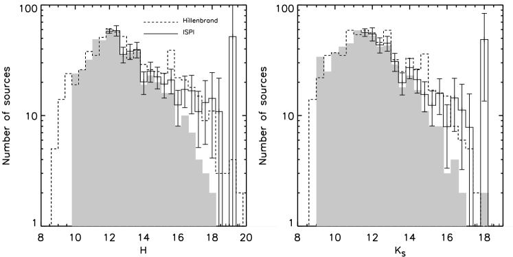
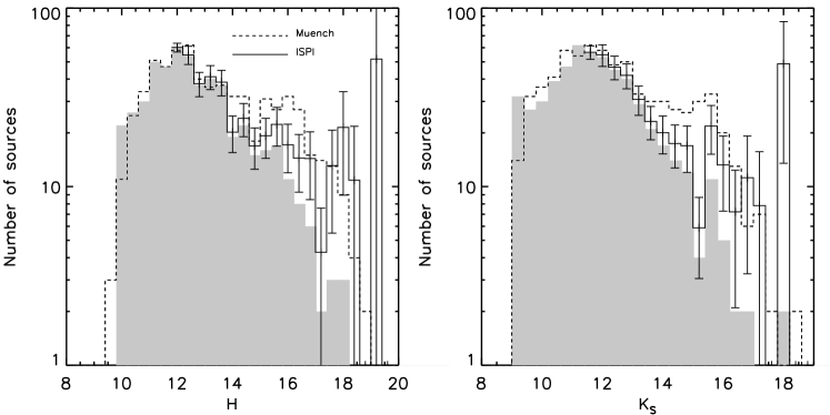
Figure 6: dashed lines: H and K_S luminosity functions for the Hillenbrand & Carpenter (2000) (upper panels) and Muench et al. (2002) (bottom panels) catalogs; gray area: luminosity functions for the same filter and fields from the ISPI observations (point sources only); solid line: ISPI luminosity functions corrected for completeness. The error bars have been obtained by adding quadratically the statistical (poissonian) uncertainty on the measured counts to the completeness correction error derived from the Monte Carlo simulations.

The results of our simulations are shown in Figure 5. For each filter, the completeness estimated in the outer region is slightly, but systematically, larger than that in the intermediate region, which in turn is much larger than in the bright inner region, the most heavily affected by crowding and diffuse emission, where our sensitivity begins to drop at HK_S $\sim 14$ mag. A comparison with Hillenbrand & Carpenter (2000) and Muench et al. (2002), who surveyed the inner part of the cluster ($5\arcmin\times 5\arcmin$ and $6\arcmin\times 6\arcmin$ fields, respectively) deriving $HK$ photometry down to our photometric limit ($\hbox{\sl K{${}_{S}$}}\sim 18$ mag), shows that we detect as point sources more than 90% of their sources (648/706 in the H-band and 657/698 in the K_S-band for Hillenbrand & Carpenter (2000) and 601/662(H) and 665/714(K_S) for Muench et al. (2002)). Figure 6, where we overplot the Luminosity Functions (LFs) obtained by Hillenbrand & Carpenter (2000) and Muench et al. (2002) (dashed lines) to our observed LFs (gray area) constructed for their same regions, confirms that the missing sources are generally fainter than $\hbox{\sl H}\hbox{\sl K{${}_{S}$}}\simeq 14$ mag (the missing bright sources, detected but not measured by ISPI due to saturation, are not relevant here). If we apply to our H and K_S LFs the appropriate completeness corrections, estimated by repeating the artificial star experiment on the same fields of Hillenbrand & Carpenter (2000) and Muench et al. (2002), our LFs  become consistent with theirs, with the exception of the secondary peak at $\hbox{\sl K{${}_{S}$}}\simeq 15.5$ mag discussed by Muench et al. (2002). In Section 6.3 we will apply the completeness corrections to the measured counts, when we will compare the LFs at various distances from the cluster center.

5 Results

Our final photometric catalog contains 7759 sources. Having visually inspected all sources, we find that 6630 can be classified as point-like sources and 933 as diffuse objects. The other 174 sources, typically brighter than $K_{S}\simeq 10$, turn out to be saturated even in our short 3 s images. We included them in our catalog, adopting the photometry and coordinates reported by 2MASS. We also found that the 2MASS photometric catalog misses 22 sources in the Trapezium region clearly visible in the 2MASS images and saturated even in our short exposures. We have added their JHK_S photometry using the Muench et al. (2002) photometry.

In Table 4 we summarize the number of sources measured in different combination of filters, exposure times, and morphological types. The source catalog, presented in Table 5, is available in the electronic edition of this paper. In Appendix A we illustrate the content of each field of the source catalog.

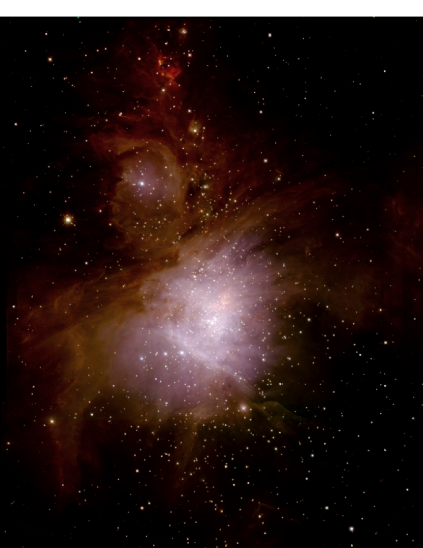
Figure 7: Near-IR color composite mosaic of the Orion Nebula from our ISPI images. The image has been digitally enhanced to improve the visibility of the stellar sources in the central region. The RGB colors code the K_S, H and J  bands, respectively.

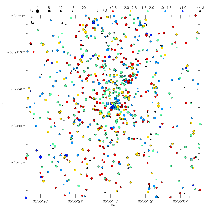
Figure 8: Spatial distribution of the ONC stars for the inner (Trapezium) region. The caption at top of the figure illustrates how the size of the circles is proportional to the source brightness, whereas the colors are from blue to red according to their observed J-K_S  index. White arrows are used to indicate the Trapezium stars, for orientation

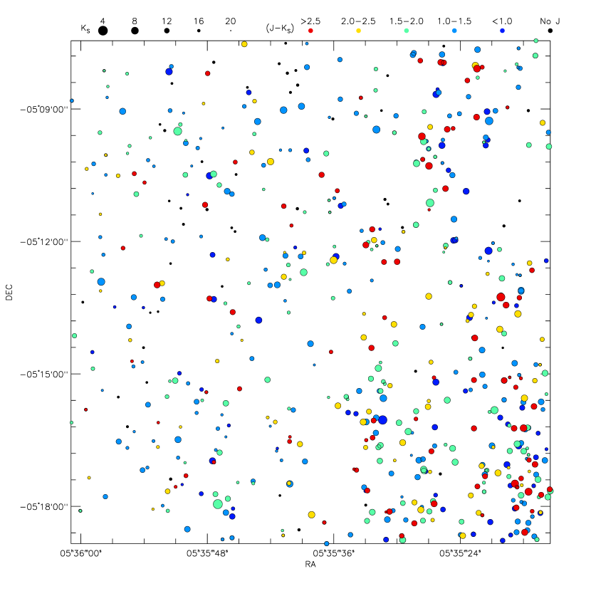
Figure 9: Same as Figure 8, for Field 1.

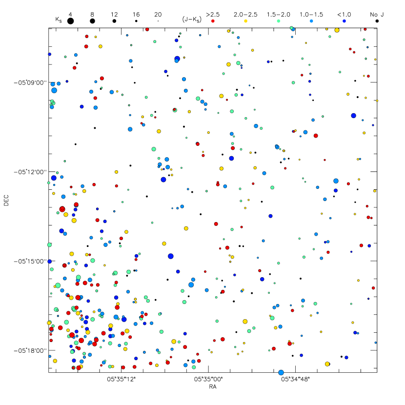
Figure 10: Same as Figure 8, for Field 2.

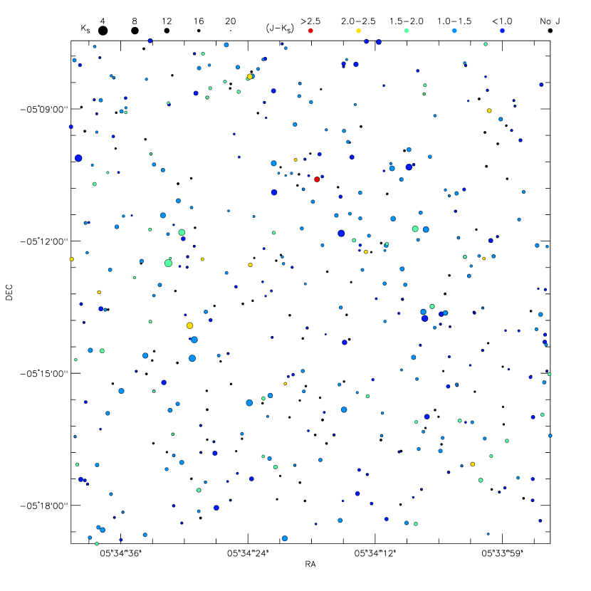
Figure 11: Same as Figure 8, for Field 3.

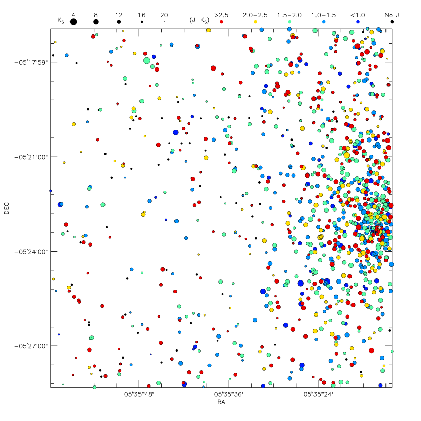
Figure 12: Same as Figure 8, for Field 4.

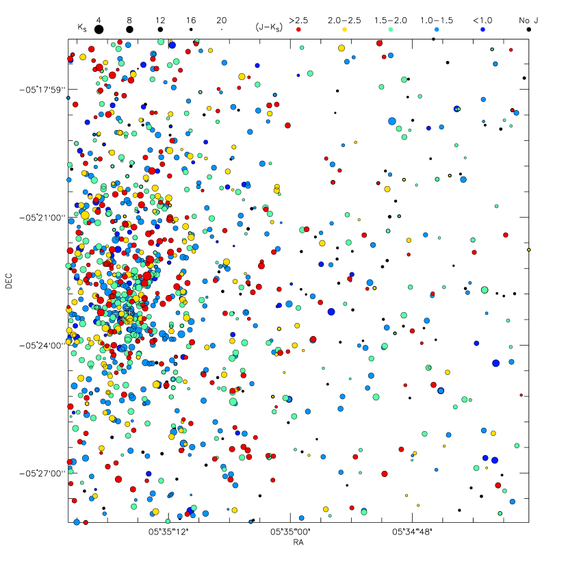
Figure 13: Same as Figure 8, for Field 5.

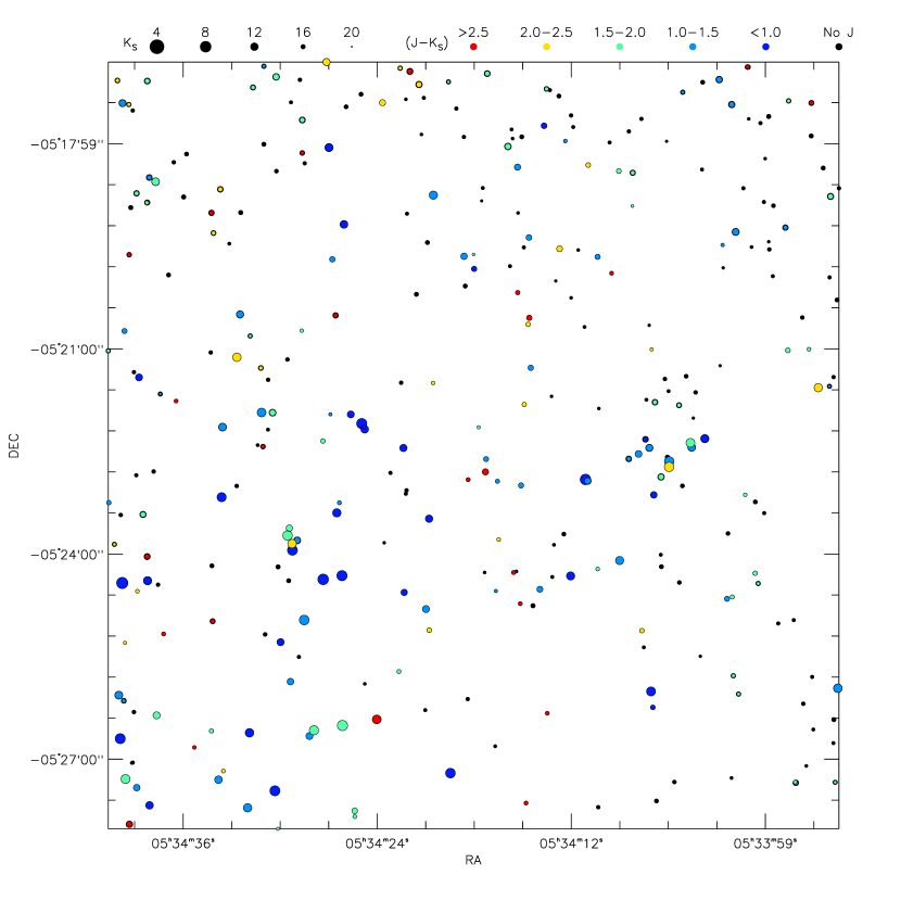
Figure 14: Same as Figure 8, for Field 6.

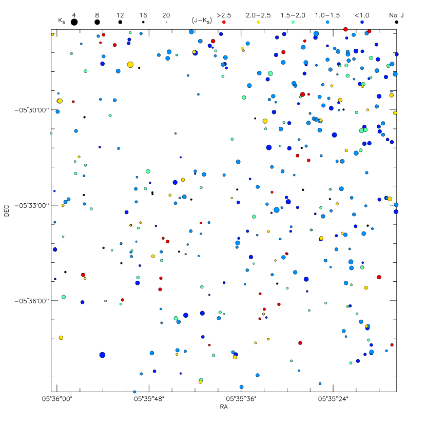
Figure 15: Same as Figure 8, for Field 7.

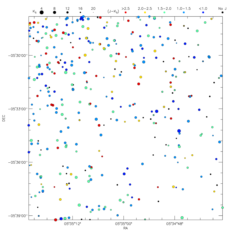
Figure 16: Same as Figure 8, for Field 8.

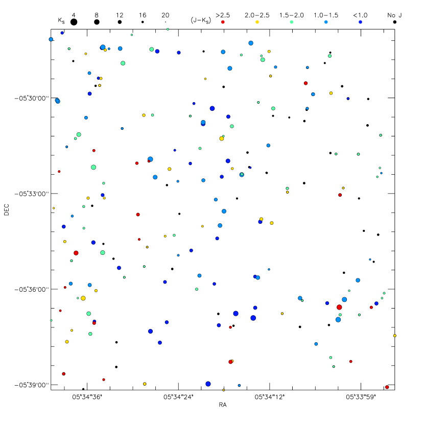
Figure 17: Same as Figure 8, for Field 9.

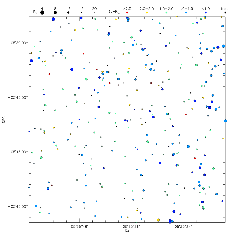
Figure 18: Same as Figure 8, for Field 10.

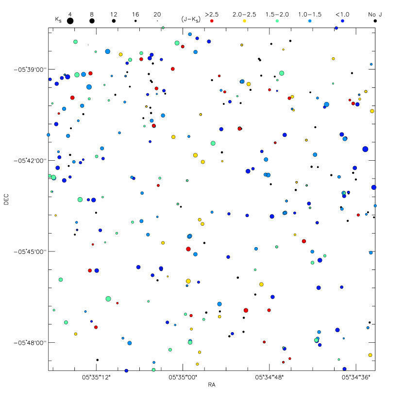
Figure 19: Same as Figure 8, for Field 11.

Figure 7 shows a JHK_S color composite of our imaged field. The image, produced by the graphic staff of the Space Telescope Science Institute, has been artificially enhanced to reduce the original dynamic range and more clearly reveal the inner part of the cluster. Figures 8-19 provide 12 finding charts, starting from the Trapezium region (Figure 8) and continuing with the 11 fields (Figure 9 to 19). The sources are coded with circles having sizes proportional to their brightness and colors scaled from blue to red according to their observed J-K_S colors.

6 Discussion

In this paper we present a preliminary analysis of the data, concentrating on the point-like sources of the Orion Nebula Cluster having the full set of JHK_S photometry with magnitude errors $\Delta m\leq 0.3$, with the exception of sources seen only in Field 3 (thus lacking the deep J exposure) and within $5^{\prime}$ from NU Ori, i.e., lying in the field of the satellite nebula M43, about $15^{\prime}$ northeast of the Trapezium. Our sub-sample is therefore composed by 4103 sources.

6.1 Color-color diagrams

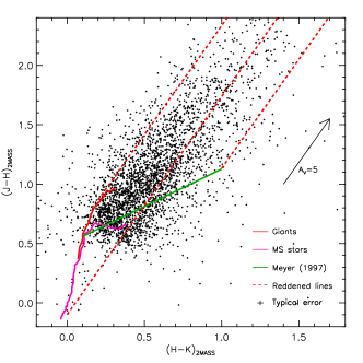
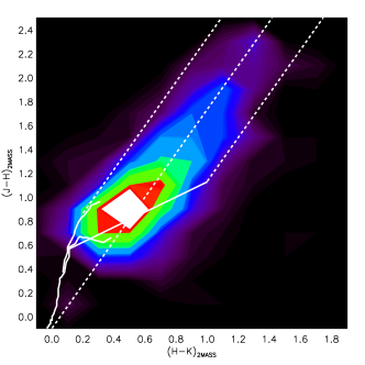
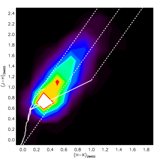
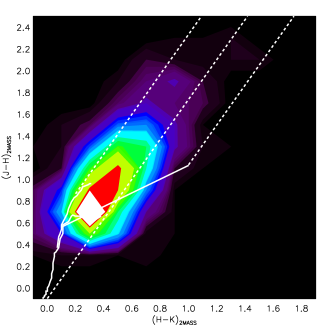
Figure 20: a) top-left panel: Near-infrared color-color diagrams for selected point-like sources in our catalog detected in all 3 bands (see text for the selection criteria). Also shown are the main-sequence (magenta solid line), the giant-branch (red solid line) sequence and the CTTs locus by Meyer et al. (1997) (green solid line). The dotted lines are parallel to the standard reddening vector. b) (top-right panel) - Hess diagrams of the color-color diagram relative to the inner region. c) bottom-left panel: Similar to panel b), for the median region. d) bottom-right panel: Similar to panel b) for the outer region.

In Figure 20a we show the near-IR J-H versus H-K_S color-color diagram. Following Lee et al. (2005), we overplot the intrinsic colors of the main-sequence stars and giant branch, together with the locus of classical T Tauri stars (CTTSs) surrounded by circumstellar disks (Meyer et al., 1997), given by the relation $(\hbox{\sl J}-\hbox{\sl H})-0.630(\hbox{\sl H}-\hbox{\sl K{${}_{S}$}})-0.497=0$ in the 2MASS photometric system. We also plot the interstellar reddening vector of Cardelli et al. (1989), given by the relation $E(\hbox{\sl J}-\hbox{\sl H})/E(\hbox{\sl H}-\hbox{\sl K{${}_{S}$}})=1.83$ in the 2MASS photometric system. Accounting for extinction, the locus of the CTTSs lies between the two parallel dotted lines defined by the equations $(\hbox{\sl J}-\hbox{\sl H})-1.83(\hbox{\sl H}-\hbox{\sl K{${}_{S}$}})+0.098=0$ and $(\hbox{\sl J}-\hbox{\sl H})-1.83(\hbox{\sl H}-\hbox{\sl K{${}_{S}$}})+0.50=0$.

For 45.2% (1853/4103) of the sources, the near-IR colors are consistent with those of stellar dwarfs (luminosity class V), giants (luminosity class III) or CTTSs reddened by various amounts of foreground extinction. For 11.4% (466/4103) of the sources the near-IR excess is compatible only with the reddened CTTSs, whereas only 0.8% (35/4103) of the sources show near-IR excess significantly greater than those of CTTSs, indicative of strong K_S-band excess.

To assess how the observed reddening and color excess vary with the distance from the center of the cluster, we consider the Hess diagrams for the three radial regions. The inner field (Figure 20b) shows a peak well detached from the main sequence, with iso-density contours elongated in a direction parallel to the CTTSs locus, together with a long tail of stars with high reddening. The Hess diagram for the intermediate region (Figure 20c) shows a main peak much closer to the locus of dwarf stars, together with a secondary maximum at higher extinction. The intermediate contour levels (e.g. the green area) are now elongated along the range of reddened main sequence stars. Finally, the Hess diagram for the outer region (Figure 20d) shows again a strong peak compatible with dwarf stars affected by a small amount of extinction, whereas the low contour levels appear less pronounced than in the two other regions and well within the limits of reddened main sequence or giant stars.

Overall, the three color-color diagrams can be interpreted as follows: 1) the inner Trapezium region is mostly populated by young stars with near-infrared excesses typical of CTTSs. They have generally relatively modest amounts of extinction, which is compatible with the fact that the ionizing radiation from the Trapezium stars has cleared the molecular cloud and exposed them to our view; 2)  the intermediate region contains a relatively larger number of heavily reddened sources. They are seen through denser parts of the OMC, not yet reached by the expansion of the ionized cavity; 3) the outer regions mostly contain background objects seen trough the low opacity layers at the edges of the main OMC ridge, which crosses the ONC approximately in north-south direction (Goldsmith et al., 1997).

6.2 Color-magnitude diagrams

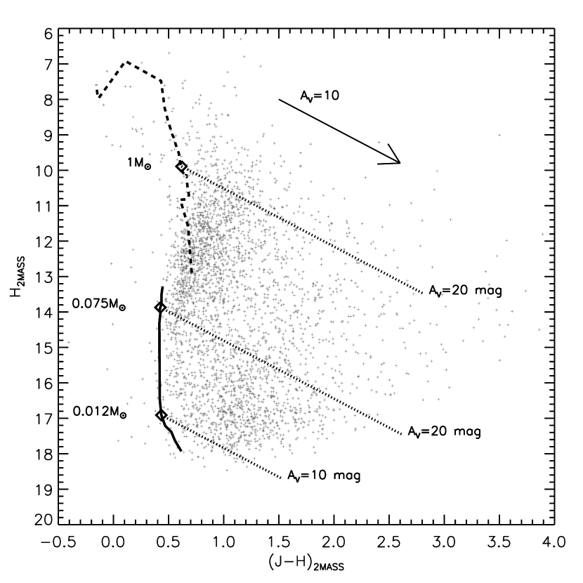
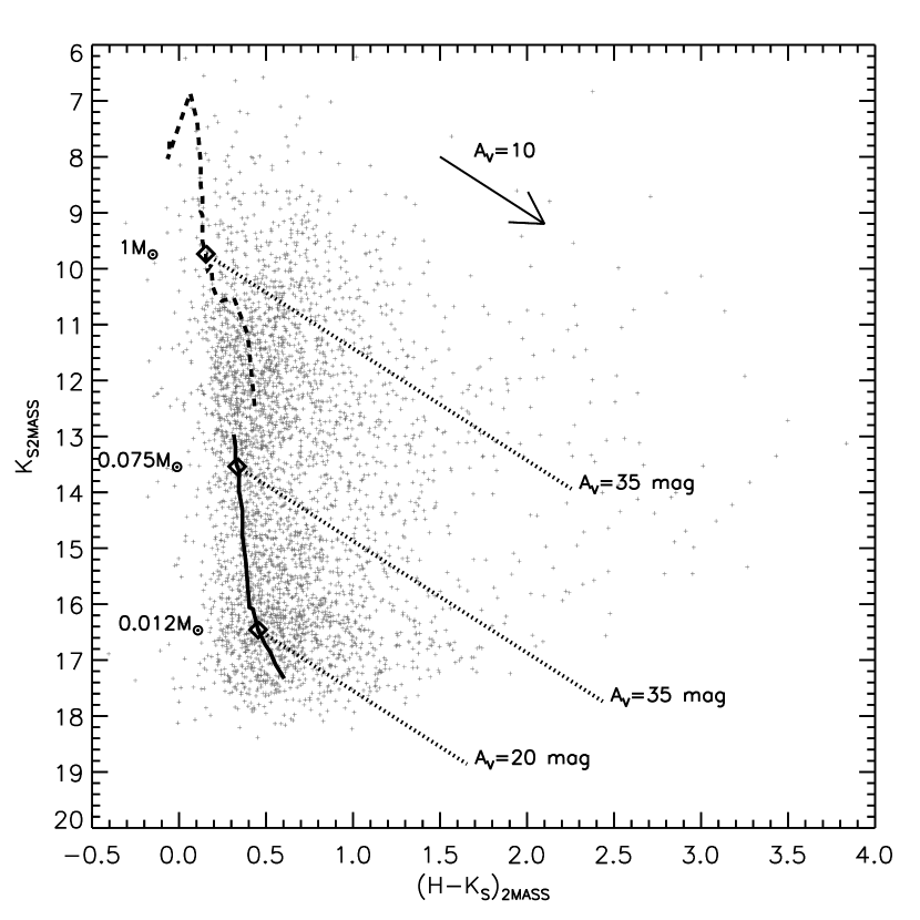
Figure 21: Infrared color-magnitude diagrams for selected point sources in our catalog detected in all 3 bands, with 1Myr isochrones, assuming a distance $d=414$ pc ($DM=8.01$). To derive these isochrones, we used (Chabrier et al., 2000) combined to the (Siess et al., 2000) model, as discussed in Section 6.2. The $A_{V}$=10 mag reddening vector is also shown. The diamond symbols represent the positions of a $M=0.012$ M_⊙ (deuterium burning limit) object, a $M=0.075$ M_⊙ (hydrogen burning limit) object and a $M=1$ M_⊙ star from bottom to top respectively.

In Figure 21 we present the (H, J-H) and (K_S, H-K_S) color-magnitude diagrams still for the same sample. Together with our data, we plot the 1 Myr isochrone of Chabrier et al. (2000, CBA00), which covers the range $0.001~{}M_{\odot}<M<0.1~{}M_{\odot}$ and is tailored to model substellar and planetary mass objects in the limit of high opacity photospheres. We also plot the 1 Myr isochrone of Siess et al. (2000, sie00) ranging from $0.1~{}M_{\odot}$ to $7~{}M_{\odot}$, well-suited for stellar sources. Both isochrones have been converted to the 2MASS photometric system using the transformations of Carpenter (2001). The offset between the two isochroness can be regarded as a graphic representation of the uncertainties in theoretical models. An $A_{V}=10$ reddening vector is also indicated, as well as the reddening lines starting from the isochrones in correspondence of a $1~{}M_{\odot}$ object (J=10.50, H=9.88 and K_S=9.76 at 414 pc in the 1Myr Sie00 isochrone), a M=0.075 $M_{\odot}$ object at the hydrogen-burning limit mass (J=14.29, H=13.86 and K_S=13.56 at 414 pc in the 1Myr CBAH00 isochrone) and a $M=0.012~{}M_{\odot}$ substellar object at the deuterium-burning limit mass (J=17.33, H=16.90 and K_S=16.48 at 414 pc in the 1 Myr CBAH00 isochrone). For this distance and isochrone, we are therefore sensitive to stellar sources down to $A_{V}\simeq 60$, brown dwarfs down to $A_{V}\simeq 40$, and planetary mass objects down to $A_{V}\simeq 15$.

Almost all data points lie to the right of the isochrones and are therefore compatible with reddened 1 Myr old sources (as well as heavily reddened field objects). If we discard the blue sources with $\hbox{\sl J}-\hbox{\sl H}<0.3$, typically affected by large measurement errors, we find that the reddening lines identify 2246 sources in the region of reddened stellar photospheres, 1298 sources in the region of reddened brown dwarfs and 142 sources in the region of reddened planetary mass objects. In the (K_S, H-K_S) color-magnitude diagrams these values are 2134, 1145, and 421, respectively.

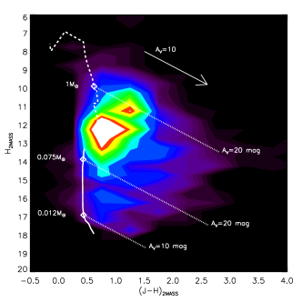
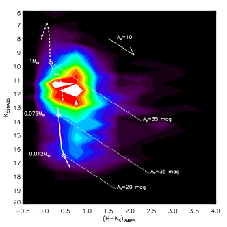
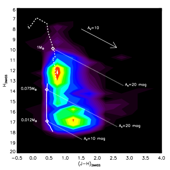
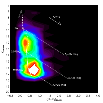
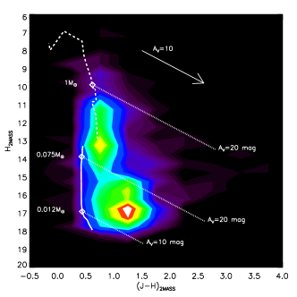
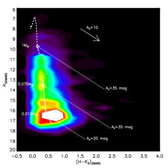
Figure 22: Hess format for the J,J-H (left panels) and K_S,H-K_S (right panels) color-magnitude diagrams. Line styles and symbols are the same as in Figure 21. From top to bottom, the diagrams for the inner ($r<6.7^{\prime}$), medium ($6.7^{\prime}<r<14.3^{\prime}$) and outer ($14.3^{\prime}<r<27.2^{\prime}$) regions are shown.

Splitting the cluster in the same three regions of Figure 4, we obtain the color-magnitude diagrams presented in Figure 22. From top to bottom, Figure 22 shows the (H, J-H) (left column) and (K_S, H-K_S) color-magnitude diagrams for the inner, median and outer regions, respectively. Consistent with what was found analyzing the color-color diagrams, the inner and outer regions appear dominated by two different populations. The top diagrams clearly reveal the location of the ONC: an ensemble of stellar sources with modest amounts of foreground extinction. The bottom diagrams are dominated by fainter sources (of course, for background stars the 1 Myr isochrone at 414 pc does not apply), whereas the intermediate region contains a mix of both populations. A careful look at the diagrams show that the peak corresponding to the ONC drifts down (i.e., to lower masses) and left (to lower extinction values) moving from the inner to the outer regions. The shift to lower masses represents an overabundance of higher mass sources at the center of the cluster, in agreement with the evidence for mass segregation found by Hillenbrand & Hartmann (1998). The redder color of the cluster members in the central field may be due to the fact that they are, on average, either more embedded in the OMC or subject to higher circumstellar extinction from their heavily warped or flared circumstellar disks (Robberto, Beckwith & Panagia, 2002), or a combination of the two.

6.3 Luminosity Functions

We conclude our analysis showing the J, H  and K_S-band luminosity functions (LFs) for all point-like sources. Once again, we remove stars less than $5^{\prime}$ projected distance from NU Ori and divide the remaining sample in three groups according to the distance criteria adopted in the previous sections. Rather than assuming a certain completeness limit, we fully apply our completeness corrections, derived in Section 4, to the source counts measured in the various regions.

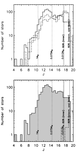
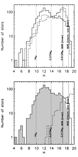
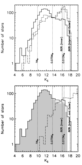
Figure 23: Top panels: J-band (left), H-band (center) and K_S-band (right) luminosity functions for the ONC, corrected for completeness. The solid line is relative to the inner region, the dashed line to the intermediate region and the dotted-dashed lines to the outer region. Bottom panels: for each bandpass, luminosity function of the inner region (solid line), of the outer region shifted by $A_{V}=33$ mag of extinction (dot-dashed line), and difference of the two (gray area). In each plot, we indicate with vertical lines the magnitudes corresponding to stars 1 Myr old at 414 pc with 1 $M_{\odot}$, 0.075 $M_{\odot}$ and 0.012 $M_{\odot}$ respectively, without interstellar reddening. The vertical dashed line stands for the 80% sensitivity level in the outer region.

The histograms for the inner region (Figure 23, thick solid line) show a broad peak at $\hbox{\sl J}\simeq 13$, $\hbox{\sl H}\simeq 12$  and $\hbox{\sl K{${}_{S}$}}\simeq 12$, corresponding to an M6 star (0.175 M_⊙) at 1 Myr, according to the Siess et al. (2000) model with zero reddening. The peak shows an abrupt drop at about $\hbox{\sl J}\hbox{\sl H}\simeq 14$ and $\hbox{\sl K{${}_{S}$}}\simeq 13$, approximately by a factor $\simeq 2$, which is fully consistent with the previous near-infrared studies of the ONC, e.g. Figure 5 of Hillenbrand & Carpenter (2000). On the other hand, the luminosity functions corrected for completeness remains remarkably flat across the substellar region down to our sensitivity limit. This is not what has been found by other authors who concentrated on the innermost area. We remark that our completeness correction has the largest effect in the inner region, the one more affected by crowding and by the brightness of the nebular background. On the other hand, we have seen that our completeness correction fails to reproduce the $\hbox{\sl K{${}_{S}$}}\simeq 14$ secondary peak of Muench et al. (2002), and for this reason can hardly be suspected of providing an artificial overcorrection in the central area.

Moving from the inner to the outer parts of our survey area, the main peak in the LFs becomes less prominent in the median region and eventually disappears in the outer regions giving to the LFs an increasing monotonic slope. If we compare our K_S-band LF for the outer cluster with the $K$-band LF of the off-cluster control field presented by Muench et al. (2002) (Figure 3a of their paper), which shows no stars brighter than $K\simeq 12$, we see that our outer field still contains a fraction of sources belonging to the cluster or, more in general, associated to the recent star formation events in the Orion region (i.e. possible foreground members of the Orion OB1 association). This is in agreement with what we found in the previous section discussing the color-magnitude diagrams, not by chance since the LF represents the projection on the vertical axis of the color–magnitude plot.

The flattening of the substellar LFs in the inner region may be due to field star contamination. To address this possibility, we can use our outer field as a control field, knowing that it will probably provide an overestimate of the contribution of non-cluster sources and therefore, after subtraction, a lower limit to the cluster LF. This for two main reasons: first, we have seen that our outer field still contains a fraction of cluster-related sources and, second, background sources should be more easily observed in the outer field rather than in the central region due to the larger background extinction caused by the underlying OMC-2, which has the ridge of highest density crossing the cluster core nearly in a north-south direction (see e.g. the extinction map obtained from the C¹⁸O column density data of Goldsmith et al. (1997) presented in Fig 2 in Hillenbrand & Carpenter (2000)). Figure 23 (bottom, gray area) shows the LFs corrected in this way, having properly normalized the source densities to the same surface area. There is a clear reduction of source density in the substellar regime and the main peak becomes more prominent, but the substellar LFs seem to remain flat or show, at best, a very modest negative slope.

Alternatively, it is possible to account for the higher background extinction beyond the central field, and therefore remove at least some of the systematic bias introduced by using the outer field, by shifting the outer LFs, for each filter, by magnitude values compatible with the interstellar reddening law of Cardelli et al. (1989). This because with a proper, wavelength dependent, change of zero points one can use the outer field counts to reproduce the luminosity functions that would have been observed with higher foreground extinction. If we refer again to the Hillenbrand & Carpenter (2000) extinction map, we see that the very central part of the OMC-2 is characterized by a visual extinction as high as $A_{V}=75^{m}$. For a detailed analysis one should account for the spatial variation of the extinction, as done e.g. by Hillenbrand & Carpenter (2000), but for the moment let’s simply assume the LFs of the outer region and put all sources under $A_{J}\simeq 10$ mag, $A_{H}\simeq 6$ mag, and $A_{K_{S}}\simeq 4$ mag, corresponding to $A_{V}\simeq 33$ mag. It is immediate to see that shifting the monotonically increasing field LFs to the right by a few magnitudes and subtracting them from the central ones produces no visible change on the central ones. One can therefore safely conclude that the true LF of the inner region lies between the one derived above subtracting the outer field source density (corresponding to a fully transparent background) and the one originally observed (corresponding to a fully opaque background), which means that the inner LFs overall remain quite flat in the brown-dwarfs regime (0.075-0.012$M_{\odot}$). In a future paper we will address the implications of this result on the cluster Inititial Mass Function, evaluating the foreground extinction and the stellar parameters of the point sources on the basis of the rich set of multicolor photometry obtained for the HST  Treasury Program on the Orion Nebula.

7 Summary and conclusions

We have presented a photometric survey of the Orion Nebula Cluster in the J-, H- and K_S-passbands carried out at the 4m telescope of Cerro Tololo. The survey, covering a field of about $30\arcmin\times 40\arcmin$ centered about $1\arcmin$ southwest of the Trapezium, has been performed in parallel to visible observations of the same region made in La Silla (Da Rio et al. 2009). The two datasets constitute the first panchromatic survey covering simultaneously the Orion Nebula Cluster from the U-band to the K_S-band.

The final catalog, photometrically and astrometrically calibrated to the 2MASS  system, contains 7759 sources, (including 174 and 22 sources whose photometry has been taken directly from the 2MASS and Muench et al. (2002) catalogs, respectively). This represents the largest near-IR catalog of the Orion Nebula Cluster to date. Our sensitivity limits allow to detect objects of a few Jupiter masses under about $A_{V}\simeq 10$ magnitudes of extinction.

We present the color-color diagrams, color-magnitude diagrams and the luminosity functions for three regions centered on the Trapezium containing the same number of sources (excluding the M43 sub-cluster). Sources in the inner region typically show IR colors compatible with reddened T Tauri stars, whereas the outer fields are dominated by field stars seen through an amount of extinction which decreases with the projected distance from the center. The color-magnitude diagrams allow to clearly distinguish between the main ONC population, spread across the full field, and background sources. After correction for completeness, the luminosity functions in the inner region remains nearly flat, with marginal contamination from background sources.

Appendix A The database

The following is a legend of the fields in the database.

1. id: Running catalog number. The 174 sources taken from the 2MASS catalog have a progressive id starting from 10,000. Sources from the Muench et al. (2002) catalog have their original entry number added to either 20,000 or 21,000, depending if the photometry was derived from FLWO or VLT observations (for sources having both measurements, the FLWO  photometry has been adopted).

2. ra: Source Right Ascension (2000.0) in decimal hours. Based on the K_S band value if the source is detected and not saturated, otherwise the H-band or the J-band, in the order.

3. dec: Source Declination (2000.0) obtained following the same priorities of the RA above.

4. raj: Right Ascension in the J band images.

5. decj: Declination in the J band images.

6. rah: Right Ascension in the H band images.

7. dech: Declination in the H band images.

8. rak: Right Ascension in the K_S band images.

9. deck: Declination in the K_S band images.

10. j: J band PSF magnitude, calibrated to the photometric 2MASS system.

11. dj: Uncertainty in the above.

12. h: H band PSF magnitude, calibrated to the photometric 2MASS system.

13. dh: Uncertainty in the above.

14. k: K_S band PSF magnitude, calibrated to the photometric 2MASS system.

15. dk: Uncertainty in the above.

16. j_ap: J band magnitude for a 5 pixel radius aperture, calibrated to the photometric 2MASS system.

17. dj_ap: Uncertainty in the above.

18. h_ap: H band magnitude for a 5 pixel radius aperture, calibrated to the photometric 2MASS system.

19. dh_ap: Uncertainty in the above.

20. k_ap: K_S band magnitude for a 5 pixel radius aperture, calibrated to the photometric 2MASS system.

21. dk_ap: Uncertainty in the above.

22. image: Image from which the measures are taken. Image numbers run from 1 to 11.

23. exptime: Set to either 3 or 30, it refers to the exposure time in seconds of the individual frames building the image from which the photometry has been taken. Sources with exptime=3 are generally saturated in the 30 s exposures.

24. status: Flag sources according to various criteria:

    • 1 : source is point-like, detected during the first photometric extraction;

    • 2 : source is point-like, detected after PSF subtraction;

    • 3 : source appears extened (galaxies, proplyds, diffuse objects in general);

25. clone: Flag for multiple detections. Sources detected multiple times have the clone value equal to the id value of their first appearance in the database, multiplied by -1.

Facilities: CTIO (ISPI)

Figure 1: Position of the eleven ISPI fields, superimposed to the positions of the sources detected in our survey.

Figure 4: Projected regions identified in our surveyed area. The solid circles define the three radial areas containing an equal number of point-like sources, with radii of 6.7′, 14.3′ and 27.2′, respectively. The dashed circle indicates the exclusion field centered around NU Ori. The positions of $\theta^{1}$ Ori-C, $\theta^{2}$ Ori and NU Ori are also indicated, together with our original field positions. The axes show the angular offsets from $\theta^{1}$ Ori-C (RA (2000.0)=$05^{h}35^{m}16.46^{s}$, DEC (2000.0)=$-05^{\circ}23\arcmin 23\farcs 18$).

Figure 5: Completeness levels for the J (left), H (center) and K_S (right) bands derived from the artificial star experiment. Each plot shows the results for the 3 radial regions.

Table 1: ISPI Broad Band Filters

Filter	Central wavelength	$\Delta\lambda(80\%$)
	($\mu$m)	($\mu$m)
J	1.250	1.176 - 1.322
H	1.635	1.500 - 1.770
KS	2.150	1.992 - 2.300

Table 2: Log of the ISPI observations

Field	Night	RA (2000.0)	DEC (2000.0)	Airmass	Comment
1	A	05:35:38.37	-5:12:50.7	1.144 - 1.291
2	A	05:34:59.63	-5:12:57.6	1.123 - 1.139
3	A	05:34:18.52	-5:12:59.6	1.123 - 1.139	no J-band 30s exposure
4	A	05:35:37.05	-5:22:38.6	1.309 - 1.158
	B	05:35:36.96	-5:22:50.6	1.309 - 1.158	field 12 in the database
5	A	05:34:59.08	-5:22:28.3	1.319 - 1.938
	B	05:34:59.21	-5:22:55.0	1.225 - 1.498	field 13 in the database
6	A	05:34:17.98	-5:22:28.3	1.319 - 1.938
	B	05:34:18.01	-5:22:55.7	1.225 - 1.498	field 14 in the database
7	B	05:35:38.16	-5:33:03.8	1.218 - 1.410
8	B	05:34:59.82	-5:33:18.6	1.104 - 1.211
9	B	05:34:18.50	-5:33:21.4	1.104 - 1.211
10	B	05:35:37.48	-5:43:06.9	1.110 - 1.215
11	B	05:34:56.28	-5:43:09.2	1.110 - 1.215

Table 3: Best estimate for calibration coefficients.

Field	$Z_{H}$	$\sigma_{Z_{H}}$	$\epsilon_{JK}$	$\sigma_{\epsilon_{JK}}$
1	1.09	0.01	-0.010	0.008
2	1.07	0.01	0.001	0.007
3	1.08	0.04	0.00	0.02
4	1.13	0.01	-0.022	0.006
5	1.11	0.01	-0.023	0.007
6	1.03	0.02	-0.05	0.02
7	0.93	0.02	0.00	0.01
8	0.93	0.01	-0.023	0.008
9	0.95	0.01	-0.02	0.01
10	1.09	0.02	-0.06	0.01
11	1.07	0.02	-0.02	0.01

Note. — Parameters for field 3 are computed using non-normalized J-band magnitudes.

Table 4: Source Summary

Source	Number of stars
ISPI detected in J-, H- and KS-bands	4851
ISPI detected in J- and H-bands, not in KS-band	92
ISPI  detected in H- and KS-bands, not in J-band	1096
ISPI detected in J- and KS-bands, not in H-band	85
ISPI detected only in J-band	175
ISPI detected only in H-band	80
ISPI detected only in KS-band	251
ISPI  diffuse	933
ISPI Total	7563
Extracted from the 2MASS catalog	174
Extracted from the Muench et al. (2002) catalog	22
Grand Total	7759
ISPI detected in 30 s images	6147
ISPI detected in 3 s images	1416
ISPI  first run detection	6305
ISPI  hidden companions	325
ISPI diffuse	933

?

Table 5: ISPI Photometry and Astrometry of the Orion Nebula Cluster

ID	RA	DEC	RAJ	DECJ	RAH	DECH	RAK	DECK	J	DJ	H	DH	K	DK	J_AP	DJ_AP	H_AP	DH_AP	K_AP	DK_AP	IMAGE	STATUS	EXPTIME	CLONE
1	5.5891618	-5.2200644	0.0000000	0.0000000	0.0000000	0.0000000	5.5891618	-5.2200644	0.00000	0.00000	0.00000	0.00000	0.00000	0.00000	0.00000	0.00000	0.00000	0.00000	14.7662	0.127338	1	30	3	0
2	5.5953268	-5.2236077	5.5953268	-5.2236077	5.5953268	-5.2236077	5.5953268	-5.2236077	0.00000	0.00000	0.00000	0.00000	0.00000	0.00000	18.3755	0.165048	17.1395	0.0658121	16.5264	0.109725	1	30	3	0
3	5.5892962	-5.2290140	5.5892962	-5.2290140	5.5892962	-5.2290140	5.5892962	-5.2290140	0.00000	0.00000	0.00000	0.00000	0.00000	0.00000	21.6719	3.20662	18.8478	0.312653	16.5874	0.435113	1	30	3	0
4	5.5957626	-5.2373337	5.5957626	-5.2373337	5.5957626	-5.2373337	5.5957626	-5.2373337	0.00000	0.00000	0.00000	0.00000	0.00000	0.00000	18.2395	0.144179	16.8748	0.0518666	16.2750	0.0847839	1	30	3	0
5	5.5977591	-5.2379900	5.5977591	-5.2379900	5.5977591	-5.2379900	5.5977591	-5.2379900	0.00000	0.00000	0.00000	0.00000	0.00000	0.00000	14.9843	0.0181128	14.1678	0.0144228	13.8639	0.0164303	1	30	3	0
6	5.5977757	-5.2385170	5.5977757	-5.2385170	5.5977757	-5.2385170	5.5977757	-5.2385170	0.00000	0.00000	0.00000	0.00000	0.00000	0.00000	16.1198	0.0362412	15.5781	0.0223180	15.1644	0.0347833	1	30	3	0
…	…	…	…	…	…	…	…	…	…	…	…	…	…	…	…	…	…	…	…	…	…	…	…	…
50	5.5892075	-5.3059220	5.5892064	-5.3059297	5.5892100	-5.3059316	5.5892075	-5.3059220	13.0184	0.0607901	11.9386	0.0319145	11.3727	0.0440246	12.8548	0.0307046	11.8450	0.0206606	11.3464	0.0269704	1	3	1	50
51	5.5884842	-5.3057194	5.5884816	-5.3056698	5.5884806	-5.3056545	5.5884842	-5.3057194	12.7213	0.0437424	11.9917	0.0212242	11.6676	0.0364081	12.6560	0.0289495	11.9254	0.0186968	11.5759	0.0257633	1	3	1	51
52	5.5919210	-5.3049874	5.5919174	-5.3049865	5.5919189	-5.3049850	5.5919210	-5.3049874	11.4727	0.0458089	10.7665	0.0297185	10.5796	0.0417144	11.4616	0.0245957	10.7047	0.0164845	10.5815	0.0225129	1	3	1	52
53	5.5919566	-5.3021426	5.5919551	-5.3021808	5.5919540	-5.3021369	5.5919566	-5.3021426	17.4306	0.218837	16.6371	0.107383	16.3148	0.208574	17.3613	0.256974	16.5880	0.123214	16.2403	0.230356	1	3	1	53
…	…	…	…	…	…	…	…	…	…	…	…	…	…	…	…	…	…	…	…	…	…	…	…	…
3597	5.5816976	-5.4131470	5.5817022	-5.4131479	5.5816945	-5.4131670	5.5816976	-5.4131470	16.7388	0.112858	16.0862	0.0527115	15.5653	0.0936435	0.00000	0.00000	0.00000	0.00000	0.00000	0.00000	5	30	2	3597
…	…	…	…	…	…	…	…	…	…	…	…	…	…	…	…	…	…	…	…	…	…	…	…	…
3678	5.5823130	-5.4152808	0.0000000	0.0000000	5.5823110	-5.4152832	5.5823130	-5.4152808	0.00000	0.00000	18.0264	0.141975	17.3747	0.147156	0.00000	0.00000	0.00000	0.00000	0.00000	0.00000	5	30	2	3678
…	…	…	…	…	…	…	…	…	…	…	…	…	…	…	…	…	…	…	…	…	…	…	…	…
4109	5.5791845	-5.3399510	5.5791916	-5.3398418	5.5791794	-5.3398919	5.5791845	-5.3399510	17.3715	0.134945	16.3929	0.0630108	15.7189	0.104973	0.00000	0.00000	0.00000	0.00000	0.00000	0.00000	5	30	2	4109
…	…	…	…	…	…	…	…	…	…	…	…	…	…	…	…	…	…	…	…	…	…	…	…	…
82996	5.5871119	-5.5159988	0.0000000	0.0000000	0.0000000	0.0000000	0.0000000	0.0000000	10.1820	0.0230000	9.26200	0.0300000	8.62400	0.0190000	0.00000	0.00000	0.00000	0.00000	0.00000	0.00000	8	0	0	82996
…	…	…	…	…	…	…	…	…	…	…	…	…	…	…	…	…	…	…	…	…	…	…	…	…
82620	5.5860662	-5.4647789	0.0000000	0.0000000	0.0000000	0.0000000	0.0000000	0.0000000	7.74300	0.0240000	7.63600	0.0470000	7.47200	0.0200000	0.00000	0.00000	0.00000	0.00000	0.00000	0.00000	8	0	0	-52620
…	…	…	…	…	…	…	…	…	…	…	…	…	…	…	…	…	…	…	…	…	…	…	…	…
81916	5.5811772	-5.5523648	0.0000000	0.0000000	0.0000000	0.0000000	0.0000000	0.0000000	8.45700	0.0320000	7.95600	0.0510000	7.85200	0.0240000	0.00000	0.00000	0.00000	0.00000	0.00000	0.00000	8	0	0	81916
…	…	…	…	…	…	…	…	…	…	…	…	…	…	…	…	…	…	…	…	…	…	…	…	…
81767	5.5797176	-5.5707202	0.0000000	0.0000000	0.0000000	0.0000000	0.0000000	0.0000000	7.22100	0.0190000	6.96400	0.0340000	6.64100	0.0180000	0.00000	0.00000	0.00000	0.00000	0.00000	0.00000	8	0	0	81767
…	…	…	…	…	…	…	…	…	…	…	…	…	…	…	…	…	…	…	…	…	…	…	…	…

Note. — Table 5 is published in its entirety in the electronic edition. A portion is shown here for guidance regarding its form and content. See Appendix A for a detailed description of the fields.

References

- Baraffe et al. (2002) Baraffe, I., Chabrier, G., Allard, F., & Hauschildt, P. H. 2002, A&A, 382, 563
- Baraffe et al. (1998) Baraffe, I., Chabrier, G., Allard, F., & Hauschildt, P. H. 1998, A&A, 337, 403
- Bertin et al. (2002) Bertin, E., Mellier, Y., Radovich, M., Missonnier, G., Didelon, P., & Morin, B. 2002, Astronomical Data Analysis Software and Systems XI, 281, 228
- Cardelli et al. (1989) Cardelli, J. A., Clayton, G. C., & Mathis, J. S. 1989, ApJ, 345, 245
- Carpenter (2001) Carpenter, J. M. 2001, AJ, 121, 2851
- Chabrier et al. (2000) Chabrier, G., Baraffe, I., Allard, F., & Hauschildt, P. 2000, ApJ, 542, 464
- Da Rio et al. (2009) Da Rio, N., Robberto, M., Soderblom, D. R., Panagia, N., Hillenbrand, L. A., Palla, F., and Stassun, K. 2009, ApJS, in press
- de Grijs et al. (2002a) de Grijs, R., Gilmore, G. F., Mackey, A. D., Wilkinson, M. I., Beaulieu, S. F., Johnson, R. A., & Santiago, B. X. 2002, MNRAS, 337, 597
- de Grijs et al. (2002b) de Grijs, R., Gilmore, G. F., Johnson, R. A., & Mackey, A. D. 2002, MNRAS, 331, 245
- de Grijs et al. (2002c) de Grijs, R., Johnson, R. A., Gilmore, G. F., & Frayn, C. M. 2002, MNRAS, 331, 228
- Goldsmith et al. (1997) Goldsmith, P. F., Bergin, E. A., & Lis, D. C. 1997, ApJ, 491, 615
- Hillenbrand (1997) Hillenbrand, L. A. 1997, AJ, 113, 1733
- Hillenbrand & Carpenter (2000) Hillenbrand, L. A., & Carpenter, J. M. 2000, ApJ, 540, 236
- Hillenbrand & Hartmann (1998) Hillenbrand, L. A., & Hartmann, L.W. 1998, ApJ, 492, 540
- Lada et al. (2008) Lada, C. J., Muench, A. A., Rathborne, J., Alves, J. F., & Lombardi, M. 2008, ApJ, 672, 410
- Landolt (1992) Landolt, A. U. 1992, AJ, 104, 340
- Lee et al. (2005) Lee, H.-T., Chen, W. P., Zhang, Z.-W., & Hu, J.-Y. 2005, ApJ, 624, 808
- Lucas & Roche (2000) Lucas, P. W., & Roche, P. F., 2000, MNRAS, 205, 361
- Lucas et al. (2005) Lucas, P. W., Roche, P. F., & Tamura, M. 2005, MNRAS, 361, 211
- Menten et al. (2007) Menten, K. M., Reid, M. J., Forbrich, J., & Brunthaler, A. 2007, A&A, 474, 515
- Meyer et al. (1997) Meyer, M. R., Calvet, N., & Hillenbrand, L. A. 1997, AJ, 114, 288
- Mink (1997) Mink, D. J. 1997, in Astronomical Data Analysis Software and Systems VI, A. S. P. Conference Series, Vol. 125, G. Hunt and H. E. Payne, eds. p. 249
- Muench et al. (2002) Muench, A. A., Lada, E. A., Lada, C. J., & Alves, J. 2002, ApJ, 573, 366
- Muench et al. (2008) Muench, A., Getman, K., Hillenbrand, L., Preibisch, T. 2008, in “Handbook of Star Forming Regions, Volume I: The Northern Sky” ASP Monograph Publications, Vol. 4. (Editor B. Reipurth), 483
- O’Dell (2008) O’Dell C. R., Muench, A., Smith, N., Zapata, L. 2008, in “Handbook of Star Forming Regions, Volume I: The Northern Sky ASP Monograph Publications”, Vol. 4. (Editor B. Reipurth), 544
- O’Dell et al. (2009) O’Dell, c. R., Henney, W. J., Abel, N. P., Ferland, G. J., and Arthur, S. J. 2009, AJ137, 367
- Persson et al. (1998) Persson, S. E., Murphy, D. C., Krzeminski, W., Roth, M., & Rieke, M. J. 1998, AJ, 116, 2475
- Press et al. (1997) Press W. H., Teukolsky S. A., Vetterling W. T., Flannery B. P. 1997, Cambridge University Press
- Rieke & Lebofsky (1985) Rieke, G. H., & Lebofsky, M. J. 1985, ApJ, 288, 618
- Robberto, Beckwith & Panagia (2002) Robberto, M., Beckwith, S. V. W., & Panagia, N. 2002, ApJ, 578, 897
- Scandariato (2008) Scandariato, G. 2008, Master Thesis, University of Catania
- Sherry (2003) Sherry, W. H. 2003, The Young Low-Mass Population of Orion’s Belt, Ph. D. Thesis, State University of New York, Stony Brook
- Siess et al. (2000) Siess, L., Dufour, E., & Forestini, M. 2000, A&A, 358, 593
- Stetson (1987) Stetson, P. B. 1987, PASP, 99, 191
- Xin-yue et al. (2009) Xin-yue, E, Zhi-bo, J., Yan-ning, F. , 2009, Chinese Astronomy and Astrophysics, 33, 139