Baryon axial charges from Chirally Improved fermions - first results

Abstract:

We present first results from dynamical Chirally Improved (CI) fermion simulations for the axial charge $G_{A}$ of various hadrons. We work with $16^{3}\times 32$ lattices of spatial extent 2.4 fm and use the variational method with a suitable basis of Jacobi-smeared interpolators to suppress contaminations from excited states.

1 Introduction

The axial charge of the nucleon, or more precisely the ratio $G_{A}(q^{2}=0)/G_{v}(q^{2}=0)$ has been determined to a high precision from neutron $\beta$ decay, with $G_{A}(0)/G_{v}(0)=1.2695(29)$. In general, the axial form factor $G_{A,BB^{\prime}}$ for an octet baryon is given by

$$\left<B^{\prime}|A_{\mu}(q)|B\right> =\bar{u}_{B^{\prime}}(p^{\prime})\left(\gamma_{\mu}\gamma_{5}G_{A,BB^{\prime}}(q^{2})+\gamma_{5}q_{\mu}\frac{G_{P}(q^{2})}{2M_{B}}\right)u_{B}(p)\mathrm{e}^{-iq\cdot x}\ ,$$ (1)

where $G_{P}$ is the induced pseudoscalar form factor. The axial charge is defined as the value of the axial form factor at zero momentum transfer $G_{A,BB^{\prime}}(q^{2}=0)$. In the following, we will omit the indices $B$ and $B^{\prime}$ when referring to the nucleon. For the nucleon in the chiral limit, the Goldberger-Treiman relation $G_{A}=F_{\pi}g_{\pi NN}/M_{N}$ connects the axial charge to the pion decay constant $F_{\pi}$, the pion-nucleon coupling constant $g_{\pi NN}$ and the nucleon mass $M_{N}$. Away from the chiral limit, this relation is still approximately fulfilled. Assuming the conservation of the vector current (which is the case for mass-degenerate light quarks $m_{u}=m_{d}$), the nucleon axial charge is also related to the polarized quark distributions in the proton: $G_{A}=\Delta u-\Delta d$ [1]. In an isovector combination, disconnected contributions cancel, making high-precision lattice computations feasible.

The Chiral Perturbation Theory ($\chi PT$) expressions relevant to the nucleon axial charge have been calculated in [2], where finite volume effects are taken into consideration. While a recent simulation with domain wall fermions [3] finds considerable finite volume effects and scaling in $M_{\pi}L$, volume effects calculated in $\chi PT$ lead to differing conclusions. Trying to attribute this difference to excited state contaminations arising from finite separation in Euclidean time, Tiburzi [4] estimates the effects of such contaminations and obtains that they would lead to an over-estimation of $G_{A}$ rather than an under-estimation. He also suggests to study $G_{A}$ using the variational method. Lattice results for the nucleon axial charge have furthermore been presented in [5]. For a recent review, please refer to the review by Renner [6].

So far, only one group has reported results for the axial couplings of sigma and cascade hyperons [7]. The corresponding $\chi$PT calculations can be found in [8]. In [9] input from experiment and lattice QCD is used to determine the unknown parameters in the $\chi PT$ expansion and predict the mass dependence and values of the axial charges in the chiral limit.

In the next section, we explain the setup for calculations of baryon axial charges using Chirally Improved (CI) lattice fermions and the variational method. We will then move on and present results from our calculations of the axial charges of the nucleon and of $\Sigma$ and $\Xi$ hyperons.

2 Details of our calculational setup

For our simulations we use CI fermions [10], which are approximate Ginsparg-Wilson fermions based on an expansion of Dirac operator terms on a hypercube. CI fermions have been tested extensively in quenched calculations [11] and results for the ground state spectrum of mesons and baryons from dynamical CI simulations have been presented recently [12].

Assuming mass-degenerate up- and down quarks it is sufficient to consider the following current insertion to extract the axial charge

$$2A_{\mu}^{3} =A_{\mu}^{u}-A_{\mu}^{d}\ ,\qquad A_{\mu}^{u}=\bar{u}\gamma_{\mu}\gamma_{5}u\ ,\qquad A_{\mu}^{d}=\bar{d}\gamma_{\mu}\gamma_{5}d\ ,$$ (2)

in which $u$ denotes an up quark and $d$ denotes a down quark. In the following, we will show how three-point functions with insertions like those in Equation 2 can be evaluated on the lattice.

Figure 1: Different possibilities for the calculation of sequential quark propagators (left and middle). The right-hand side shows an illustration of the full baryon three-point function.

For our calculations we use so-called sequential propagators. In [1], two methods for the calculation of sequential quark propagators are presented. Figure 1 illustrates these two approaches. On the left-hand side, sequential sources are built from specific diquark propagators, while in the middle, the propagators are calculated for each possible insertion separately. An illustration of the full baryon three-point function is provided on the right-hand side. Which approach is computationally cheaper depends on the physics objective. In our case, we want to use two different insertions and two widths of smearing for three different interpolator types. As we are using a rather coarse lattice, a small number of insertion timeslices should be enough. Therefore, even when just considering the nucleon case, the second approach using sequential sources from single quark propagators is slightly cheaper. Moreover, these propagators can subsequently be used for other hadrons and for the calculation of transition form factors.

To relate lattice operators, which receive a finite renormalization, to their continuum counterparts, we need to estimate the renormalization factors $Z_{\Gamma}$ of the bilinear currents in question. In general, we have to multiply the lattice result $G_{\Gamma}^{lat}$ by the appropriate renormalization factor to obtain values that can be compared with results extracted from experiments

$$G_{\Gamma}^{phys}=Z_{\Gamma}G_{\Gamma}^{lat},$$ (3)

which are typically given in the modified minimal subtraction ($\overline{MS}$) renormalization scheme.

For dynamical CI fermions, these renormalization constants have been estimated using local bilinear quark field operators in [13]. It would however be useful to have an independent estimation of these constants from a different method. In the case of the vector current, one can estimate the constant $Z_{V}$ by calculating the vector charge $G_{V}$ defined in analogy with (1) via

$$\left<B^{\prime}|V_{\mu}(q)|B\right> =\bar{u}_{B^{\prime}}(p^{\prime})\left(\gamma_{\mu}G_{V}(q^{2})+q_{\nu}\sigma_{\nu\mu}\frac{G_{T}(q^{2})}{2M_{B}}\right)u_{B}(p)\mathrm{e}^{-iq\cdot x}\ ,$$ (4)

as $G_{V}(q^{2}=0)$. This quantity has to be 1 in the continuum, as it is related to the electric charge of the proton in the limit of equal quark masses [1].

For lattice fermions with exact chiral symmetry, the axial vector renormalization constant $Z_{A}$ and the vector renormalization constant $Z_{V}$ have to be equal. For lattice fermions which only fulfill the Ginsparg-Wilson relation approximately, there should be small deviations from this. To obtain an independent estimate of $Z_{V}$, we use a ratio of two-point over three-point functions [14]

$$R^{(k)} =\frac{\sum_{l}\sum_{m}\psi_{l}^{(k)}C(t)_{lm}\psi_{m}^{(k)}}{\sum_{i}\sum_{j}\psi_{i}^{(k)}T_{V}(t,t^{\prime})_{ij}\psi_{j}^{(k)}}=Z_{V}\ ,$$ (5)

where $C(t)$ is the matrix of two-point correlation functions and $T_{V}(t,t^{\prime})$ is the matrix of three-point correlators with a vector insertion. The eigenvectors $\psi$ are the ones obtained from a variational analysis of $C(t)$. We then compare with the preliminary estimates from [13]. The ensemble names are according to [12], where details of the run parameters are provided. For runs A and B the two methods agree within $2-3\%$. While a determination using local quark bilinears yields 0.818(2) for run A and 0.826(1) for run B, we find values for $Z_{V}$ of 0.803(2) and 0.792(2) respectively. For run C there is a rather large discrepancy and the method of [13] leads to a value of 0.829(1) while we obtain 0.77(1). Notice also that two different methods for the determination of the renormalization constants are presented in [13] which only agree after a chiral extrapolation of the results is performed. At the same time, the ratio $Z_{A}/Z_{V}$ determined from the values in [13] is almost identical for both methods used and also stable under chiral extrapolation of the results.

In our determination of the axial charge from run C, we encounter what we suspect to be large finite volume effects. Notice that the value of $Z_{V}$ obtained from the nucleon three-point functions might be plagued by the same effects. As we cannot calculate $Z_{A}$ from baryon three-point functions, we therefore always use the ratio $Z_{A}/Z_{V}$ from [13]. In the next section, we discuss in detail which ratios we measure on the lattice to obtain the renormalized axial charge $G_{A}$.

3 Nucleon axial charge from dynamical CI fermions

The usual approach [1, 3] is to extract the nucleon axial charge from ratios of $G_{A}$ over $G_{V}$

$$G_{A} =\frac{Z_{A}}{Z_{V}}\frac{T_{A}^{3}(t,t^{\prime})}{T_{V}(t,t^{\prime})}\ ,$$ (6)

using single correlation functions built from either smeared quarks or gauge fixed box or wall sources. This approach has the advantage that some of the systematic errors entering the lattice determination will cancel.

We instead use the variational method, which is commonly used to extract ground and excited state masses. It is based on a correlation matrix $C_{ij}(t)=\langle O_{i}(t)O^{\dagger}_{j}(0)\rangle$ where $O_{i}(t)$ are operators with the quantum numbers of the state of interest. The eigenvalues $\lambda_{i}$ of the generalized eigenvalue problem $C(t)v_{i}=\lambda_{i}C(t_{0})v_{i}$ may be shown to behave as $\lambda_{i}(t)\propto\mathrm{e}^{-tE_{i}}\left(1+\mathcal{O}\left(\mathrm{e}^{-t\Delta E_{i}}\right)\right)$, where $E_{i}$ is the energy of the $i$-th state. The approach may be generalized to three point functions. Following [14], we obtain an expression for $G_{A}$:

$$G_{A} =\frac{Z_{A}}{Z_{V}}\frac{\sum_{i}\sum_{j}\psi_{i}^{(k)}T_{A}^{3}(t,t^{\prime})_{ij}\psi_{j}^{(k)}}{\sum_{l}\sum_{m}\psi_{l}^{(k)}T_{V}(t,t^{\prime})_{lm}\psi_{m}^{(k)}}\ .$$ (7)

Figure 2 shows a typical plateau for the axial charge of the nucleon from run C extracted from such a ratio. The horizontal lines denote the results from a linear fit in the displayed range. Notice that we observe a plateau in the full range of points we calculated. For all three ensembles, we choose timeslice $t$ = 9 for the position of the sink. This corresponds to a source-sink separation of roughly $1.2\,\mathrm{fm}$. For run B, we currently only have data for insertion timeslices $t^{\prime}$ from 5 to 9. Instead of assuming that the central value at 5 is the physical one, we perform a linear fit in the range 5 to 7.

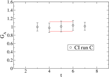
Figure 2: Example plot to illustrate typical plateaus observed with our variational basis for a source-sink separation of $\approx 1.2\,\mathrm{fm}$. The data is from run C.

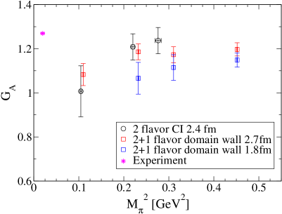
Figure 3: We compare our results for $G_{A}$ to a recent determination from domain wall fermions. Our data is labeled as “2 flavor CI”. Results from 2+1 flavor domain wall fermions are taken from Yamazaki et al. [3]. On the left-hand side, we plot the results over $M_{\pi}^{2}$. Towards lower quark masses finite volume effects are clearly visible. On the right-hand side we display our data in units of $M_{\pi}L$.

We compare our data to recent results from domain wall fermions [3] in Fig. 3. The left-hand side plot shows the results for $G_{A}$ plotted over the square of the pion mass $M_{\pi}^{2}$. While results at large pion masses lead to values close to the experimental value, the result from run C deviates substantially from this behavior. The same is true for the domain wall data and this behavior seems to be a universal feature associated with finite volume effects [3, 6]. On the right-hand side of the figure we therefore plot the results for $G_{A}$ over $M_{\pi}L$, where $L$ corresponds to the spatial extent of the lattice. This plot can be directly compared to Fig. 3 of [3].

Before we move on to calculations for hyperons, let us briefly comment on the sink-dependence of our results. While results from run A and B are rather insensitive to the sink location in the region explored (timeslices 9-13), a systematic shift upwards can be observed for run C when reducing the separation between the source and the sink from 8 to 6 timeslices which corresponds to distances of $1.2\,\mathrm{fm}$ and $0.9\,\mathrm{fm}$. We want to point out that this does not affect the quality of the plateau which still stretches over the entire region of insertion times. Taking a look at the nucleon two point functions, contributions from excited states to the ground state of the variational analysis are visible up to timeslice 4. This is an indication that excited states may indeed be responsible for measuring a larger value of $G_{A}$ if excited state contributions are not sufficiently suppressed. With just 50 configurations, the statistical errors from our preliminary dataset are by far too large to make a stronger and more quantitative statement.

4 Hyperon axial charges

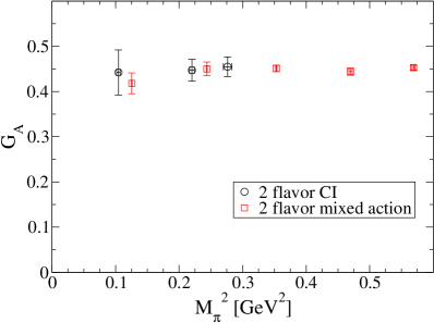
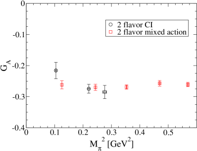
Figure 4: Results for the axial charges of the $\Sigma$ (left-hand side) and $\Xi$ (right-hand side) hyperons compared to the mixed action results by Lin and Orginos [7].

In this section we present results for a calculation of hyperon axial charges. For the $\Sigma$ and $\Xi$ hyperons we adopt the following definitions:

$$\left<\Sigma^{+}|A_{\mu}^{3}|\Sigma^{+}\right>-\left<\Sigma^{-}|A_{\mu}^{3}|\Sigma^{-}\right>=G_{\Sigma\Sigma}\;\bar{u}^{\nu}\gamma_{\mu}\gamma_{5}u^{\nu}\ ,$$ (8)

$$\left<\Xi^{0}|A_{\mu}^{3}|\Xi^{0}\right>-\left<\Xi^{-}|A_{\mu}^{3}|\Xi^{-}\right>=G_{\Xi\Xi}\;\bar{u}^{\nu}\gamma_{\mu}\gamma_{5}u^{\nu}\ .$$ (9)

Again, no disconnected contributions appear in the isovector quantities and the calculation proceeds similar to the nucleon case. In particular, no additional sequential propagators are needed.

Figure 4 shows our results for the axial charges of the $\Sigma$ and $\Xi$ hyperons. We compare our data to [7] and we can see a quantitative agreement in the full range of masses. Unlike for the nucleon, no significant decrease is observed towards the chiral limit in the plot for the $\Sigma$ (l.h.s.). The plot for the $\Xi$ (r.h.s.) also shows a nice agreement with the results from [7]. In this case our value corresponding to the smallest pion mass shows a slight decrease towards the chiral limit, but the error bars are large and this may as well be an effect of our limited statistics. Our purely statistical errors on the preliminary dataset of 50 configurations are still large but can be substantially reduced by using our full statistics.

5 Summary and outlook

We have presented preliminary results from a calculation of baryon axial charges using a full variational basis to efficiently suppress contaminations from excited states. We used a basis of baryon interpolators with different Dirac structures and two different smearing widths for the quarks. The results are in good agreement with the literature and we obtain clear plateaus for ratios calculated with the method of [14]. Provided the signal for the states in question is strong enough, this method can also be applied to several other quantities of interest, among them the axial charge of the delta baryon and the $N$-$\Delta$ or $\Sigma$-$\Lambda$ transition.

In general, the method we use can also be applied to three-point functions involving excited states, provided that the signal is good enough to ensure the necessary separation between the source/sink and the current insertion.

- [1] S. Sasaki, K. Orginos, S. Ohta, and T. Blum, Phys. Rev. D68, 054509 (2003).
- [2] S. R. Beane and M. J. Savage, Phys. Rev. D70, 074029 (2004); W. Detmold and C. J. D. Lin, Phys. Rev. D71, 054510 (2005).
- [3] RBC+UKQCD Collaboration, T. Yamazaki et al., Phys. Rev. Lett. 100, 171602 (2008).
- [4] B. C. Tiburzi, Phys. Rev. D80, 014002 (2009).
- [5] S. N. Syritsyn et al., PoS LATTICE2008, 169 (2008); LHPC Collaboration, R. G. Edwards et al., Phys. Rev. Lett. 96, 052001 (2006); T. T. Takahashi and T. Kunihiro, Phys. Rev. D78, 011503 (2008).
- [6] D. Renner, PoS LATTICE2009, (2009). To be published.
- [7] H.-W. Lin and K. Orginos, Phys. Rev. D79, 034507 (2009).
- [8] F.-J. Jiang and B. C. Tiburzi, Phys. Rev. D77, 094506 (2008); B. C. Tiburzi and A. Walker-Loud, Phys. Lett. B669, 246–253 (2008).
- [9] F.-J. Jiang and B. C. Tiburzi, arXiv:0905.0857.
- [10] C. Gattringer, D63, 114501 (2001); C. Gattringer, I. Hip, and C. B. Lang, Nucl. Phys. B597, 451–474 (2001).
- [11] BGR Collaboration, C. Gattringer et al., Nucl. Phys. B677, 3–51 (2004).
- [12] C. Gattringer et al., Phys. Rev. D79, 054501 (2009); C. B. Lang et al., PoS LATTICE2009, 088, (2009).
- [13] P. Huber unpublished, 2009.
- [14] T. Burch, C. Hagen, C. B. Lang, M. Limmer and A. Schäfer, D79, 014504 (2009).