Self-calibration of photometric redshift scatter in weak lensing surveys

Abstract

Photo-z errors, especially catastrophic errors, are a major uncertainty for precision weak lensing cosmology. We find that the shear-(galaxy number) density and density-density cross correlation measurements between photo-z bins, available from the same lensing surveys, contain valuable information for self-calibration of the scattering probabilities between the true-z and photo-z bins. The self-calibration technique we propose does not rely on cosmological priors nor parameterization of the photo-z probability distribution function, and preserves all of the cosmological information available from shear-shear measurement. We estimate the calibration accuracy through the Fisher matrix formalism. We find that, for advanced lensing surveys such as the planned stage IV surveys, the rate of photo-z outliers can be determined with statistical uncertainties of $0.01$-$1\%$ for $z<2$ galaxies. Among the several sources of calibration error that we identify and investigate, the galaxy distribution bias is likely the most dominant systematic error, whereby photo-z outliers have different redshift distributions and/or bias than non-outliers from the same bin. This bias affects all photo-z calibration techniques based on correlation measurements. Galaxy bias variations of $O(0.1)$ produce biases in photo-z outlier rates similar to the statistical errors of our method, so this galaxy distribution bias may bias the reconstructed scatters at several-$\sigma$ level, but is unlikely to completely invalidate the self-calibration technique.

1 Introduction

Weak gravitational lensing is emerging as one of the most powerful probes of dark matter, dark energy [1] and the nature of gravity at cosmological scales [18]. In less than a decade after first detections [3, 22, 36, 38], the lensing measurement accuracy and dynamical range have been improved dramatically (e.g. Fu et al. 7). Future weak lensing surveys have the potential to measure the lensing power spectrum with sub-$1\%$ statistical accuracy for many multipole $\ell$ bins. However, whether we can fully utilize this astonishing capability is up to the control over various systematic errors. They could arise from uncertainties in theoretical modeling, including the non-linear evolution of the universe [8, 9, 10] and the influence of baryons [37, 40, 19, 30]. They could also arise from uncertainties in the lensing measurement. An incomplete list includes the galaxy intrinsic alignment [12, 24, 13, 27, 28], influence of the telescope PSF [11, 25], photometric redshift (photo-z) calibration errors [23, 6], etc. Precision lensing cosmology puts stringent requirements on calibrating these errors [15].

Weak lensing surveys are rich in physics and contain information beyond the cosmic shear power spectrum [5, 45]. This bonus allows for self-calibration of weak lensing systematic errors, such as the galaxy intrinsic alignment [45, 20]. In the present paper, we utilize the galaxy density-shear cross-correlation and density-density correlations in photometric survey data to self-calibrate the photo-z scatters between redshift bins. Namely, for a given photo-z bin, we want to figure out (reconstruct) the fraction of galaxies which are actually located in a distinct redshift bin. These scatters quantitatively describe the photo-z outliers or catastrophic errors. The effect of photo-z outliers on cosmological inference from the shear-shear power spectrum is discussed by Bernstein & Huterer [6], which also quantifies the task of calibrating these outliers by direct spectroscopic sampling of the galaxy population. Since spectroscopic sampling of faint galaxies at $>99\%$ completeness is an expensive or infeasible task for current ground-based capabilities, Newman [26] proposes a technique based on cross-correlation between the photo-z sample and an incomplete spectro-z sample.

Here we ask a complementary question: how well can the outlier rate be determined using purely photometric data from the original lensing survey? As pointed out by Schneider et al. [32], the spurious cross correlation between the galaxy density in two photo-z bins can be explored to calibrate photo-z errors. They found that, for a photo-z bin of the size $\Delta z=0.5$ in a LSST-like survey, $1\%$ level scatters can be identified and the mean redshift can be calibrated within the accuracy of $\sim 0.01$. This result is impressive. Unfortunately, a factor of $10$ improvement is still required to meet the statistical accuracy of those ambitious “stage IV” projects ($\sim 10^{-3}$, Huterer et al. 15). In combination with baryon acoustic oscillation and weak lensing measurements, the constraints can be significantly improved [42]. However, these procedures adopt a number of priors/parameterizations, which may bias the calibration.

A successful self-calibration should not correlate cosmological uncertainties with astrophysical uncertainties (in our case, photo-z errors). To meet this requirement, the self-calibration should adopt as few cosmological priors as possible, preferably none. On the other hand, it should not result in loss of cosmological information. In this paper, we propose to combine the galaxy-galaxy clustering measurement and shear-galaxy cross correlation measurement to perform the photo-z self-calibration, strictly reserving the shear-shear measurement for cosmology. Finally, it must be able to reach sufficiently high statistical accuracy and have controllable systematics, if any. As we will show, this self-calibration meets all the three requirements and is able to detect scatters as low as $0.01\%$.

There are a number of differences between our self-calibration method and the method proposed by Schneider et al. [32]. (1) The inclusion of shear-galaxy cross correlation measurement breaks a severe degeneracy in the previous method and thus significantly improves the calibration accuracy. (2) We do not adopt any parameterizations on the photo-z probability distribution function (PDF) and are thus free of possible bias induced by improper parameterizations. (3) This method is a true self-calibration, in the sense that the photo-z scatters are reconstructed solely from the given weak lensing surveys, no external measurements nor priors on cosmology and galaxy bias, are needed. (4) We argue that the shot noise is the only relevant noise term for the likelihood analysis. Sample variance and non-Gaussianity, do not affect the reconstruction. This allows us to go deeply into the nonlinear regime, gain many more independent modes for the reconstruction, and significantly improve the reconstruction accuracy.

Like most of these predecessor papers, we analyze an idealized survey: apparent density fluctuations induced by gravitational lensing are ignored; galaxy biasing is assumed to be common to all galaxies at a given redshift; and shear measurement errors are ignored. Incorporation of these and other effects can substantially degrade the correlation-based photo-z calibration methods [6]. A framework for comprehensive analysis of photometric$+$spectroscopic lensing survey data is presented in Bernstein [5], and is necessary to make a final judgment on the efficacy of photo-z self-calibration. However this complicated analysis has not yet been applied to the problem of photo-z outlier calibration. The simpler analysis presented here will demonstrate that the galaxy-shear and galaxy-galaxy correlations contain sufficient information to measure the outlier rate to useful precision, and we will then examine the possibility of degradation by the non-ideal effects.

This paper is organized in the following way. In §2, we describe our self-calibration technique and target a fiducial “Stage IV” lensing survey for the error forecast. We discuss in §3 possible systematic errors which can be incorporated into our technique and will not bias the photo-z PDF reconstruction. Other systematic errors cannot be self-calibrated without strong priors or external information. For these, we quantify the induced bias in §4. We further discuss uncertainties in the error forecast due to uncertainties in the fiducial model and the robustness of our self-calibration technique (§5). We discuss possibilities to improve the calibration accuracy (§6). We also include two appendices (§A & B) for technical details of the Fisher matrix analysis and bias estimation.

2 Photo-z self-calibration

We first define several key notations used throughout the paper.

• The superscript “P” denotes the property in the photo-z bin.

• The superscript “R” denotes the corresponding property in the true-z bin.

• The capital “G” denotes gravitational lensing, to be more specific, the lensing convergence converted from the more direct observable cosmic shear.

• The little “g” denotes galaxy number density (or over-density).

We split galaxies into $N_{z}$ photo-z bins. The $j$-th photo-z bin has the range $[z_{j}-\Delta z_{j}/2,z_{j}+\Delta z_{j}/2)$. Our notation is that larger $i$ means higher photo-z. $N_{j}$, the total number of galaxies in the $j$-th photo-z bin, is an observable. We also have $N_{z}$ true-z bins, with the choice of redshift range identical to that of the photo-z bins. We denote $N_{i\rightarrow j}$ as the total number of galaxies in the $j$-th photo-z bin which also belong to the $i$-th true-z bin, namely, whose true redshift fall in $[z_{i}-\Delta z_{i}/2,z_{i}+\Delta z_{i}/2)$. The process $i\rightarrow j$ is similar to scatters (transitions) between different quantum states. So we often call this process as the photo-z scatter. The scatter rate is related to the the photo-z probability distribution function, $p(z|z^{P})$, by the following relation

$$N_{i\rightarrow j}=\int_{z_{j}-\frac{\Delta z_{j}}{2}}^{z_{j}+\frac{\Delta z_{j}}{2}}n(z^{P})dz^{P}\left[\int_{z_{i}-\frac{\Delta z_{i}}{2}}^{z_{i}+\frac{\Delta z_{i}}{2}}p(z|z^{P})dz\right]\ .$$ (1)

Here, $n(z^{P})dz^{P}$ is the number distribution of galaxies in the photo-z space. We define $p_{i\rightarrow j}\equiv N_{i\rightarrow j}/N_{j}$, which represents the averaged $p(z|z^{P})$ over the relevant redshift ranges, or the binned photo-z PDF. In the limit that $\Delta z_{i,j}\rightarrow 0$, $p_{i\rightarrow j}\rightarrow p(z_{i}|z^{P}_{j})$. Since $\sum_{i}p_{i\rightarrow j}=1$, we have $N_{z}(N_{z}-1)$ independent $p_{i\rightarrow j}$. These $p_{i\rightarrow j}$ together represent a non-parametric description of the photo-z PDF $p(z|z^{P})$ and completely describe the scattering probabilities between redshift bins, namely the rate of photo-z outliers, or leakage rate. In Bernstein & Huterer [6], they are called “contamination” coefficients.

Scatters in photo-z, especially catastrophic photo-z errors, cause a number of spurious correlations between photo-z bins. Our proposal is to reconstruct all $p_{i\rightarrow j}$ from these cross correlations. For convenience, we will work on the corresponding cross power spectra throughout the paper, instead of the cross correlation functions.

We use fiducial power spectra, fiducial leakage $p_{i\rightarrow j}$ and the survey specification to perform the error forecast. To generate the fiducial power spectra, we adopt a flat $\Lambda$CDM cosmology with $\Omega_{m}=0.27$, $\Omega_{\Lambda}=1-\Omega_{m}$, $\Omega_{b}=0.044$, $\sigma_{8}=0.84$ and $h=0.71$. The transfer function is obtained using CMBFAST [33]. The nonlinear matter power spectrum is calculated using the fitting formula of Smith et al. [35]. Unless specified, we adopt a fiducial galaxy bias $b_{g}=1$. We are then able to calculate the galaxy power spectra and lensing-galaxy power spectra. The calculation of these power spectra is by no mean precise, due to the simplification of $b_{g}=1$. However, this simple bias model suffices for the purpose of this paper, namely, to demonstrate the feasibility of our self-calibration technique. We will further investigate the impact of scale dependent bias in §5, where we find that our self-calibration technique is also applicable.

Figure 1: The fiducial $z^{P}$-$z^{S}$ scatters adopted for the forecast. The simulated data [6] has $177210$ galaxies. To control the size of the figure, we only show $2\%$ of them, randomly chosen Although there are indeed $0.7\%$ galaxies at $z^{P}>4$, in the analysis we have taken the freedom to disregard these galaxies. To make the analysis closed, we shall adopt the approximation that no galaxies with $z^{P}<4.0$ comes from $z^{S}>4.0$. We check that galaxies with $z^{S}>4.0$ only account for a tiny fraction of the whole $z^{P}<4$ sample ($0.06\%$) and even smaller fraction for low photo-z bins ( and thus not showing up in this figure since we only plot $2\%$ of all galaxies). So this approximation is sufficiently accurate for the purpose of this paper.

We also need the galaxy distribution $n(z^{P})$ and the input of fiducial $p_{i\rightarrow j}$. Due to uncertainties in survey specifications, we will not focus on any specific survey. Instead, we will target a fiducial lensing survey with some characteristics of “Stage IV” lensing surveys like LSST, Euclid and JDEM. The analysis can be redone straightforwardly to incorporate changes in the survey specifications. We follow Huterer et al. [15], Zhan & Knox [43] and adopt the photo-z distribution $n(z^{P})dz^{P}=x^{2}\exp(-x)dx/2$, where $x\equiv z^{P}/z_{0}$. For such a distribution, the median redshift is $z_{m}=2.675z_{0}$. We adopt $z_{0}=0.45$, the mean galaxy surface density $\bar{n}_{g}=40$ per arcmin², and the fractional sky coverage $f_{\rm sky}=0.5$. The rms dispersion in the shear measurement induced by the galaxy intrinsic ellipticities is adopted as $\gamma_{\rm rms}=0.2$.

The fiducial $p(z|z^{P})$ and $p_{i\rightarrow j}$ are calculated from the simulated data of Bernstein & Huterer [6], which were produced using the method described in Jouvel et al. [21]. The $z^{P}$-$z^{S}$ distribution in this data is shown in Fig. 1, where $z^{S}$ is the spectroscopic redshift, which can be approximated as the true redshift. This simulated data is for SNAP-like space weak lensing surveys, conducted in 8 broad bands spanning $0.38$-$1.7$$\mu$m wavelength. These surveys have near-IR bands and hence likely smaller photo-z errors than LSST. Since we find that the statistical accuracy of the photo-z reconstruction is not very sensitive to the choice of fiducial photo-z PDF and since photo-z calibration has room to improve, the adopted photo-z PDF should be a good representative case to illustrate our method.

Furthermore, the accuracy of the self-calibration is sensitive to the choice of redshift bins. Unless otherwise specified, we will adopt eight redshift bins, $[0.0,0.5)$, $[0.5,1.0)$, $[1.0,1.5)$, $[1.5,2.0)$, $[2.0,2.5)$, $[2.5,3.0)$, $[3.0,3.5)$ and $[3.5,4.0)$. For comparison, we also investigate the case of much finer redshift bins, $[0.0,0.1)$, $[0.1,0.2)$, $\ldots$, $[1.7,1.9)$, $[1.9,2.2)$, $[2,2,2.6)$, $[2.6,3.0)$, $[3.0,4.0)$. We call these coarse bins and fine bins, respectively. We have utilized the freedom in the data analysis and disregarded the galaxies with $z^{P}>4.0$. These galaxies only account for $0.7\%$ of the total galaxies. Neglecting them does not result in significant loss of information. On the other hand, these $z^{P}>4$ galaxies may have large photo-z catastrophic errors (Fig. 1). Neglecting them helps to reduce systematic errors.

To close the scattering process, we need to assume that no galaxies with $z^{P}<4.0$ come from $z^{S}>4.0$. Under this apssumption, what our self-calibration technique actually does, is to assign those $z^{S}>4$ galaxies into the $[3.5,4.0)$ true-z bin, instead of randomly assigning them elsewhere. We argue that this approximation is sufficiently accurate, for two reasons. First, in the simulated $z^{S}-z^{P}$ data we used, the total fraction of galaxies with $z^{P}<4.0$ and $z^{S}>4.0$ is only $0.06\%$. Second, about $90\%$ of them leak into the $[3.5,4.0)$ photo-z bin. Although the contamination rate in this redshift bin is high ($4.8\%$), the induced error in lensing modelling is small, since the lensing weighting kernel varies slowly at $z\sim 4$. Contaminations to other photo-z bins are much smaller. These $z^{S}>4$ galaxies account for $0.01\%$ of total galaxies in the $[0.0,0.5)$ photo-z bin, $0.02\%$ in the $[0.5,1.0)$ and $[3.0,3.5)$ photo-z bins. In the adopted simulated data, we detect no such galaxies in photo-z bins $\in[1.0,3.0)$. Due to these tiny fractions, mis-assignment of these galaxies is not a limiting factor of our self-calibration technique.

2.1 Galaxy-galaxy clustering

Photo-z errors, especially catastrophic errors, induce non-zero galaxy-galaxy correlation between different redshift bins, which should vanish at sufficiently small scale, where the Limber approximation holds. This set of correlations has been explored to perform the photo-z self-calibration [32]. With the presence of photo-z scatters, the measured galaxy surface density in a given photo-z bin is the combination of the corresponding ones in the true redshift bins,

$$\delta_{i}^{\Sigma,P}=\sum_{k}p_{k\rightarrow i}\delta^{\Sigma,R}_{k}\ .$$ (2)

The galaxy power spectrum between the $i$-th and $j$-th photo-z bins is

$$C^{gg,P}_{ij}=\sum_{km}p_{k\rightarrow i}p_{m\rightarrow j}C_{km}^{gg,R}\simeq\sum_{k}p_{k\rightarrow i}p_{k\rightarrow j}C_{kk}^{gg,R}\ .$$ (3)

The last equation has approximated $C_{k\neq m}^{gg,R}=0$, which holds under the Limber approximation. At sufficiently large angular scales, the Limber approximation fails and the intrinsic cross correlation $C_{k\neq m}^{gg,R}\neq 0$. For this reason, we exclude the modes with $\ell<100$. We will further discuss this issue later in the paper (§3.3).

Figure 2: Diagnostics of photo-z errors. Scatters between redshift bins caused by photo-z errors induce non-zero correlations $C^{gg,P}_{i\neq j}$ and $C^{Gg,P}_{i<j}$, which otherwise vanish. Here $i,j=1,2\ldots$ denote different redshift bins, the larger the $i,j$, the higher the redshift. These spurious cross correlations serve as diagnostics of photo-z scatters. We show the resulting $C^{gg,P}_{24}$ and $C^{Gg,P}_{23}$. The errorbars shown are from the shot noise. As explained in the text, this is the only relevant source of error.

If the relevant photo-z scatters are sufficiently large, $C^{gg,P}_{i\neq j}$ will dominate the associated shot noise. In this case, the relevant photo-z scatters become detectable. For the adjacent bins ($|i-j|=1$), the dominant contribution to $C^{gg,P}_{ij}$ obviously comes from $p_{i\rightarrow j}$ and $p_{j\rightarrow i}$, unless the corresponding $p_{i\rightarrow j}$ and $p_{j\rightarrow i}$ are tiny, which is unlikely. For correlations between non-adjacent photo-z bins, this may not be true. In Fig. 2, we show the result of $C^{gg,P}_{24}$. In this case, the dominant contribution comes from $C^{gg,R}_{33}$, through the scatters $3\rightarrow 2$ and $3\rightarrow 4$. Due to the huge sky coverage of the fiducial stage IV lensing survey, even though the signal $C^{gg,P}_{24}$ is suppressed by a huge factor ($\simeq p_{3\rightarrow 2}\times p_{3\rightarrow 4}$) relative to $C^{gg,R}_{33}$, it still overwhelms the shot noise and becomes observable.

However, an intrinsic degeneracy encoded in the galaxy-galaxy clustering significantly limits the accuracy of this approach. From Eq. 3, it is clear that the correlation $C^{gg,P}_{i\neq j}$ can be induced by a nonzero $p_{i\rightarrow j}$ or by a non-zero $p_{j\rightarrow i}$. In other words, $C^{gg,P}_{ij}(\ell)$ ($i\neq j$) only measures the combination $p_{j\rightarrow i}p_{j\rightarrow j}C^{gg,R}_{jj}(\ell)+p_{i\rightarrow i}p_{i\rightarrow j}C^{gg,R}_{ii}(\ell)$. Thus with measurement at a single multipole $\ell$ bin, the galaxy clustering measurement alone can not break this degeneracy between up and down scatters. Adding more $\ell$ bins can break this degeneracy—if the ratio $C^{gg,R}_{jj}/C^{gg,R}_{ii}$ varies with $\ell$. If for example the 3D galaxy power spectrum is a strict power-law over the relevant scales at the relevant redshift range, whose power index does not vary with redshift, then all $C^{gg}_{ii}(\ell)$ are self-similar and the solution remains degenerate. Observationally, departures from a power law have been found in the galaxy correlation function [39], so galaxy clustering measurements at many $\ell$ bins can break the above degeneracy. Nevertheless, galaxy correlation functions are observed to be close to power laws. This degrades the reconstruction accuracy. Furthermore, the slope depends weakly on galaxy type. If one uses the slight deviations from a power law, small changes in the slope of the leaking population could lead to large systematic reconstruction errors. This is an example of the galaxy distribution bias that we will scrutinize in §4.1. We will further investigate this issue in §5.

In the next section, we will show that, due to the unique geometry dependence of gravitational lensing, the degeneracy between up and down scatters is broken naturally by adding the lensing-galaxy correlation, resulting in significant improvement in the reconstruction.

2.2 Lensing-galaxy correlations

Galaxy-galaxy lensing brings $N_{z}^{2}$ new observables for each angular scale, which could be used to break the previous degeneracy. The scatter can render the otherwise vanishing foreground lensing-background galaxy cross correlation non-zero ($C^{Gg,P}_{i<j}\neq 0$). More importantly, lensing, due to its geometry dependence, distinguishes up-scatters from down-scatters. This new piece of information is the key to significantly improve the photo-z self-calibration.

Without loss of generality, we will work on the lensing convergence $\kappa$, instead of the more direct observable cosmic shear $\gamma$, which are locally equivalent in Fourier space. With the presence of photo-z scatters, the measured lensing convergence in a given photo-z bin is some linear combination of the ones in true-z bins weighted by the scatter probability,

$$\kappa_{i}^{P}=\sum_{k}p_{k\rightarrow i}\kappa^{R}_{k}\ .$$ (4)

The cross correlation power spectrum between the lensing convergence in the $i$-th photo-z bin and the galaxy number density in the $j$-th photo-z bin is given by

$$C^{Gg,P}_{ij} = \sum_{k\geq m}p_{k\rightarrow i}p_{m\rightarrow j}C_{km}^{Gg,R}\ .$$ (5)

In the absence of lensing magnification bias, $C_{km}^{Gg,R}\neq 0$ only when the source redshifts are higher than the galaxy redshifts (namely, $k\geq m$). Discussion of magnification bias and other errors will be postponed to §3 and §4.

We show in Fig. 2 the case of $C^{Gg,P}_{23}$ as an example. It is mainly contributed by $C^{Gg,R}_{32}$ through the scatters $3\rightarrow 2$ and $2\rightarrow 3$, by $C^{Gg,R}_{22}$ from the scatters $2\rightarrow 3$ and by $C^{Gg,R}_{33}$ from the scattering $3\rightarrow 2$. Given the strength of $p_{3\rightarrow 2}$ and $p_{2\rightarrow 3}$, the resulting $C^{Gg,P}_{23}$ is sufficiently large to overwhelm the shot noise at $\ell<10^{4}$. We notice that, depending on the values of the relevant $p$ and the size of the redshift bin, the dominant contribution can come from the $C^{Gg,R}_{i=j}$ term, despite the heavy suppression in its amplitude due to the low amplitude of the lensing kernel over the relevant redshift range.

In most of the cases, $C^{Gg,P}$ can not be measured with comparable accuracy to that of $C^{gg,P}$ (however, refer to Fig. 2 for one exception). However, we point out that it is valuable to include this piece of information in the photo-z self-calibration. It turns out to be the key to breaking the strong degeneracy between up and down scatters. Look at the configuration $i\geq k>j$. The scatter $i\rightarrow j$ contributes to $C^{Gg,P}_{jk}$, while the scatter $j\rightarrow i$ does not. For this reason, it can break the degeneracy between $i\rightarrow j$ and $j\rightarrow i$, encountered in the self-calibration based on galaxy clustering alone. The discriminating power relies on the intrinsic asymmetry between up and down scatters in generating the lensing effect. So it remains efficient, even in the case of self-similar $C^{gg}_{ii}(\ell)$ , where the self-calibration based on galaxy clustering alone blows up (§5).

2.3 The photo-z self-calibration combining the galaxy-galaxy and lensing-galaxy measurements

Counting degrees of freedom suggests that we should be able to perform a rather model-independent self-calibration without any priors. Mathematically, we need to solve Eq. 3 & 5 for all $p_{j\rightarrow i}$, $C^{gg,R}_{i=j}$ and $C^{Gg,R}_{i\geq j}$ simultaneously. At the beginning of this process, $C^{gg,P}$ and $C^{Gg,P}$ should be replaced with the corresponding measurements. The reconstructed power spectra $C^{gg,R}$ and $C^{Gg,R}$ contain valuable information on cosmology and can be further explored. The reconstructed $p_{i\rightarrow j}$ can then be applied to the shear-shear correlation measurement to correct for bias induced by photo-z scatters and infer the correct cosmology. In the present paper, we will focus on only $p_{i\rightarrow j}$. Thus we treat $C^{gg,P}$ and $C^{Gg,P}$ as nuisance parameters to be marginalized over.

The unknown parameters to be determined simultaneously by our self-calibration technique are $\lambda=(p_{\mu\rightarrow\nu},C^{Gg,R}_{ij}(\ell_{1}),C^{gg,R}_{kk}(\ell_{1})\ldots)$, with $\mu\neq\nu$, $i\geq j$ and $\mu,\nu,i,j,k=1,\ldots,N_{z}$. For $N_{\ell}$ multipole $\ell$ bins and $N_{z}$ redshift bins, we have $N_{z}(N_{z}+3)N_{l}/2+N_{z}(N_{z}-1)$ quantities to solve ($N_{\ell}N_{z}$ for $C^{gg,R}_{kk}$, $N_{\ell}N_{z}(N_{z}+1)/2$ from $C^{Gg,R}_{km}$ ($k\geq m$) and $N_{z}(N_{z}-1)$ for $p_{k\rightarrow m}$). On the other hand, we have $N_{\ell}N_{z}(3N_{z}+1)/2$ independent measurements of correlations. $N_{\ell}N_{z}^{2}$ of them come from $C^{Gg,P}_{ij}$ and $N_{\ell}N_{z}(N_{z}+1)/2$ from $C^{gg,P}_{i\leq j}$.

The equations to solve are quadratic in $p_{i\rightarrow j}$ and linear in $C_{ij}$ (Eq. 3 & 5). For this reason, to guarantee a unique solution for $p_{i\rightarrow j}$, the number of measurements should be at least $N_{z}(N_{z}-1)$ larger than the number of unknowns. This condition is satisfied when $N_{\ell}\geq 2$. If all the equations ( Eq. 3 & 5) are independent then $N_{\ell}=2$ is the minimum requirement. If some of the equations are linear combinations of the others, we will need $N_{\ell}>2$. For example, if the galaxy power spectra are strict power laws in $\ell$, then even perfect measurements of $C^{gg}(\ell)$ at all $\ell$ and redshift bins cannot break the degeneracies in $p$ and the self-calibration fails. In reality, none of the galaxy power spectra and shear-galaxy power spectra is strictly power law and we expect a valid self-calibration barring another unforeseen degeneracy. Furthermore, the baryon oscillations leave features in $C^{gg}$ and $C^{Gg}$, which help to improve the reconstruction accuracy [41].

To better understand the self-calibration process, we recast it as a mathematical problem to assign galaxies with photo-z labels into correct subsets (true-z bins), based on the cross correlation measurements. The condition $C^{gg,R}_{i\neq j}=0$ tells us that these subsets do not overlap with each other in true redshift. The condition $C^{Gg,R}_{i<j}=0$ sets the correct order of these true-z bins, ranking from low to high redshifts, since only galaxies behind a lens can be lensed. Furthermore, the measured power spectra have different dependences on $C^{R}$ and $p_{i\rightarrow j}$ (linearly on $C^{R}$ while quadratically on $p_{i\rightarrow j}$). This implies the possibility to separate $p$ from $C^{R}$.

However, careful readers may have already noticed a puzzling behavior. Eq. 3 & 5 are invariant under the scaling

$$p_{k\rightarrow i} \rightarrow f_{k}^{-1}p_{k\rightarrow i}\ ,$$

$$C^{gg,R}_{kk} \rightarrow f_{k}^{2}C^{gg,R}_{kk}\ ,$$ (6)

$$C^{Gg,R}_{km} \rightarrow f_{k}f_{m}C^{Gg,R}_{km}\ ,$$

where $f_{k}$ are some arbitrary constants. This seems to imply that we are not able to determine $p_{i\rightarrow j}$ without knowing $C^{gg,R}$ and $C^{Gg,R}$. However, this is not a real degeneracy. The reason is that we have the conditions $\sum_{k}p_{k\rightarrow i}=1$. These $N_{z}$ constraints uniquely fix the $N_{z}$ freedom of $f_{k}$. In the Fisher matrix analysis carried out in the next section, we enforce the conditions $\sum_{k}p_{k\rightarrow i}=1$ by explictly setting $p_{i\rightarrow i}=1-\sum_{k\neq i}p_{k\rightarrow i}$.

The above solution to this puzzling problem also leads to the solution of another question. Can we choose more true-z bins than photo-z bins in the self-calibration technique? The answer is no. In such case, the number of unknown constants $f_{k}$ is larger than the number of constraints $\sum_{k}p_{k\rightarrow i}=1$. Thus we are not able to uniquely fix $f_{k}$ and thus $p_{k\rightarrow i}$.

The absence of degeneracy in the self-calibration is, in the end, confirmed by the stability of our Fisher matrix inversion (below) for all the configurations that we have checked, including both the coarse bins and fine bins, various $n(z^{P})$ and $p(z|z^{P})$.

Figure 3: The forecasted error in $p_{i\rightarrow j}$ for the fiducial stage IV lensing survey. The labels in the plots are the photo-z bins. The horizontal axis is the true redshift. The filled circles are the results including both galaxy-galaxy correlations and shear-galaxy correlations. The open squares only use information in galaxy-galaxy correlations. We only show the cases with $i\neq j$, since $p_{i\rightarrow i}$ is not independent. The horizontal coordinate is $z_{i}$, the middle point of the $i$-th photo-z bin, instead of the averaged true redshift $\langle z_{i}\rangle$.

We thus believe that our photo-z self-calibration does work. It does not rely on any assumption of the underlying photo-z PDF. Furthermore, it does not rely on cosmological priors, since all cosmology-dependent quantities (e.g. the galaxy-galaxy and lensing-galaxy power spectra) are self-calibrated simultaneously. So the reconstructed $p$ is independent of uncertainties in cosmology. In the next section, we will quantify the reconstruction error and show that the proposed self-calibration is indeed powerful. For these reason, it can be and should be applied to ongoing and proposed weak lensing surveys such as CFHTLS, DES, LSST, JDEM and Euclid.

Before quantifying the reconstruction accuracy, we want to address a fundamental limitation of this self-calibration technique. It is designed to diagnose scatters between redshift bins. It is thus completely blind to photo-z errors which do not cause such scatter. Any one-to-one mapping between photo-z and true-z preserves $C^{gg,P}_{i\neq j}=0$ and cannot be discriminated using galaxy-galaxy correlations. Some such photo-z errors can cause $C^{Gg,P}_{i<j}\neq 0$, so we still have some discriminating power left. If, however, the mapping between photo-z and true-z is monotonically increasing, then we have $C^{gg,P}_{i\neq j}=0$ and $C^{Gg,P}_{i<j}=0$, and our self-calibration technique completely lacks the capability to detect such a photo-z error. One simple example is $z^{P}=(1+\epsilon)z$, where $\epsilon$ is a constant. We must rely on spectroscopic redshift measurements to diagnose such errors. In other words, our method can determine only the scattering matrix of photo-z’s, and is insensitive to any recalibration of the mean photo-z’s. In this paper, we assume no such mean photo-z error exists. This is certainly a crucial point of further investigation.

Figure 4: The error in the true mean redshift of each photo-z bin for the fiducial stage IV lensing survey. The filled circles are the results including both galaxy-galaxy correlations and shear-galaxy correlations. The open squares only use information in galaxy-galaxy correlations, where we can see the significant improvement by adding the shear-galaxy measurements. The results are plotted against the middle-point of the corresponding photo-z bin. We caution that the galaxy number density weighted true-z, $\langle z_{i}\rangle$, can differ significantly from the middle-point of the corresponding photo-z bin, mainly due to significant fractions of scatter into distant redshift bins. For example, for the photo-z bin $[3.5,4.0)$, $\langle z_{8}\rangle=2.97$, for $[3.0,3.5)$, $\langle z_{7}\rangle=2.7$ and for $[0.0,0.5)$, $\langle z_{1}\rangle=0.426$.

2.4 Error estimation

We derive the likelihood function and adopt the Fisher matrix formalism to estimate the capability of our self-calibration technique. The details are presented in the appendices A & B. We want to highlight that the error estimation here is distinctly different from that in routine exercises of cosmological parameter constraints and that in Schneider et al. [32]. In these cases, the theory predicts the ensemble average power spectra, which are then compared to the data. An inevitable consequence of any power-spectrum determination is uncertainty due to cosmic (sample) variance. But in our self-calibration, the cosmic variance does not work in this way, because the $C^{R}$ are fitted parameters, not theoretical predictions. What enters into the key equations 3 and 5 is not the ensemble average of the power spectra, but the actual values in the observed cosmic volume, i.e. they are the sums of their ensemble averages and cosmic variances within the observed volume. Galaxies in the same true-z bin (but different photo-z bins) share the same cosmic volume, thus their power spectra share the same sample variance (however, see §4.1 for complexities), as do their cross power spectra with the matter. Such coherence has been pointed out by Pen [29] and has been applied to improve the weak lensing measurement [29] and primordial non-Gaussianity measurement through two-point galaxy clustering [34]. Furthermore, we do not rely on a cosmological theory to predict these power spectra. Instead, our self-calibration reconstructs the actual power spectra in the observed survey volume. For this reason, the only relevant source of noise in writing down the likelihood function is the shot noise.

Figure 5: The dependence of reconstruction error on the size of redshift bins. The filled circles are the results showing in the previous figure adopting coarse redshift bins and the open circles adopt finer redshift bins. Changes in redshift bin size not only change the level of noise and the strength of signal, but also the number of parameters to be fitted. Along with the complicated error propagation, we see a quite irregular dependence on the bin size.

This point is of crucial importance for our error analysis. (1) It allows us to derive the likelihood function robustly in essentially all $\ell$ range. It is simply Gaussian, thanks to the central limit theorem and the stochasticity of shot noise. This is even true for the high-$\ell$ regime, where the underlying density fields are highly nonlinear and non-Gaussian, but the shot noise remains Gaussian over many independent $\ell$ modes. (2) Since we do not rely upon any theoretical model for the power spectra, we do not need a theory capable of predictions at small scales where non-linear and baryonic physics are important. (3) For these reasons, we do not need to disregard those $\ell$ measurements in highly nonlinear regime, as Schneider et al. [32] did. The inclusion of these measurements significantly improves the $p$ reconstruction, especially for low redshift bins. This explains much of the difference between the reconstruction errors of this paper from that of Schneider et al. [32], using the galaxy clustering measurement alone. The high-$\ell$ limit of this analysis will ultimately depend upon other limitations such as the applicability of the weak-lensing approximation at small scales, which can in principle render the adopted fiducial power spectra unrealistic and thus the error forecast unrealistic. However, in our exercise, we expect and have numerically confirmed that the contribution of high-$\ell$ is highly suppressed by the shot noise (as can be seen from Fig. 2), so the reconstruction accuracy is not sensitive to the high-$\ell$ limit. Throughout this paper, the results shown are based on the choice of $100<\ell<10^{5}$. (4) It significantly simplifies the matrix inversion and improves the numerical accuracy. For $N_{z}\sim 10$ and $N_{l}\sim 100$, the Fisher matrix to invert is several thousand by several thousand. However, a dominant portion of this Fisher matrix is block diagonal, due to the shot noise feature of the error sources. This allows us to significantly reduce the work on matrix inversion. The detail is explained in the appendix.

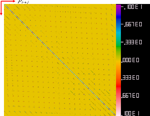
Figure 6: The cross correlation coefficient between errors in $p$. To demonstrate the fine structure, we choose the fine redshift bins ($N_{z}=22$ redshift bins in total). Both the horizontal and vertical axes are $p_{i\rightarrow j}$ ($i\neq j$), which runs with the order $(i,j)=(2,1),(3,1),\ldots,(N_{z},1),(1,2),(3,2)\ldots,(N_{z},2),\ldots$. There are 462 $p$s in total. Errors in $p_{i\rightarrow j}$ and $p_{k\rightarrow j}$ are correlated, since they could cause some $C^{Gg,P}\neq 0$. Errors in $p_{i\rightarrow j}$ and $p_{i\rightarrow k}$ are correlated too, since they cause $C^{gg,P}_{jk}\neq 0$. More fine structure can be found by zooming in this figure.

We show the error forecast in Figs. 3, 4, 5 & 6. For most bins at $z<2$, $p$ can be reconstructed to accuracy $<0.01$, for either coarse or fine bins. The improvement by adding the shear-galaxy measurement is often better than $30\%$, up to a factor of a few. We can also compress errors in $p_{i\rightarrow j}$ into a single number $\sigma_{\langle z\rangle}$, the statistical error in the mean true redshift of each photo-z bin. $\sigma_{\langle z\rangle}$ by no means captures all information of the reconstruction error, but it is a convenient reference. The result of $\sigma_{\langle z\rangle}$ for coarse bins is shown in Fig. 4 and that for fine bins is shown in Fig. 5. For the coarse bins, it can reach $O(10^{-3})$ for $z<2$. The improvement by adding the lensing-galaxy measurement is a factor of $\sim 10$ at $z<2$, mainly through the improvement in constraining scatters from high redshift bins. $\sigma_{\langle z\rangle}$ for fine bins is larger (Fig. 5). However, these errors are tightly anti-correlated, as can be inferred from Fig. 5 and 6. This is the reason we see big improvement when choosing bigger bin size.

We present an order of magnitude estimation to understand these numbers of the reconstruction error. For example, many $p_{i\rightarrow j}$ can be determined within the accuracy of $O(10^{-4})$. We take ${p_{2\rightarrow 1}}$ as an example. The scatter $2\rightarrow 1$ causes $C^{gg,P}_{12}\neq 0$. Ignoring other scatters, the threshold of $p_{2\rightarrow 1}$ is roughly set when the accumulated signal-to-noise of the $C^{gg,P}_{12}$ measurement is 1,

$$\left(\frac{S}{N}\right)_{12}^{2}\sim\sum_{\ell}\left(\frac{C^{gg,P}_{12}}{\sigma^{gg}_{12}}\right)^{2}=p_{2\rightarrow 1}^{2}\sum_{\ell}\left(\frac{C^{gg,R}_{22}}{\sigma^{gg}_{12}}\right)^{2}=1\ .$$ (7)

Here, $\sigma$ is the associated shot noise power spectrum. We find that the threshold $p_{2\rightarrow 1}$ inferred from the above equation is even smaller than $\sigma_{p_{2\rightarrow 1}}$, the statistical error in $p_{2\rightarrow 1}$ (Fig. 3). This is indeed expected. Due to simplifications made in the derivation, mainly the neglect of error propagation from other $p_{i\rightarrow j}$ and $C_{ij}$, the threshold of $p_{2\rightarrow 1}$ obtained from the above approximation is certainly a lower limit of $\sigma_{p_{2\rightarrow 1}}$.

From similar arguments, we also expect that the statistical errors for $p_{i\rightarrow j}$ are large for those high redshift bins (e.g. $i=7,8$), because the number of galaxies in these high redshift bins is small and thus the shot noise is large. However, as explained early, $C^{gg,P}$ is not the only source of information for the $p$ reconstruction. $C^{Gg,P}$ can also play important role. For example, the reconstruction of $p_{1\rightarrow 8}$ can reach an accuracy of $10^{-4}$. The reason is that the scatter $1\rightarrow 8$ causes $C^{Gg,P}_{1j}\neq 0$. The combined G-g measurements have $S/N>1$ even for $p_{1\rightarrow 8}=10^{-4}$. The $C^{gg,P}_{18}$ measurement also contributes, but since the number of galaxies in the $8$-th bin is only 1% of total galaxies, the associated shot noise is large. So its contribution is overwhelmed by that from $C^{Gg,P}_{1j}$ ($j<8$). This explains the factor of 10 improvement in the $p_{1\rightarrow 8}$ reconstruction when adding the G-g measurements. Finally, we caution that, although we are able to qualitatively explain some results of Fig. 3, the error prorogation is complicated and the above estimation only serves as a convenient tool to understand Fig. 3.

$\delta p_{i\rightarrow j}$, the errors in $p_{i\rightarrow j}$, are correlated, and the correlations show rich structures. To better demonstrate these features, we adopt the fine redshift bins, $N_{z}=22$ in total. We define the cross correlation coefficient between $\delta p$, as $r_{i_{1}j_{1};i_{2}j_{2}}\equiv\langle\delta p_{i_{1}\rightarrow j_{1}}\delta p_{i_{2}\rightarrow j_{2}}\rangle/\sqrt{\langle\delta p_{i_{1}\rightarrow j_{1}}^{2}\rangle\langle\delta p_{i_{2}\rightarrow j_{2}}^{2}\rangle}$. The resulting $r$ is shown in Fig. 6. Strong positive and negative correlations exist for errors between many scatters into the same photo-z bins ($p_{i\rightarrow j}$ and $p_{k\rightarrow j}$, regions around the diagonal of Fig. 6). These scatters are coupled since both reduce $C^{Gg}_{j<m}\neq 0$ ($i>m$ and $k>m$) or $C^{Gg}_{m<j}$ ($m>i$ and $m>k$). Scatters $i\rightarrow j$ and $i\rightarrow k$ are coupled, too, since they contribute to $C^{gg,P}_{jk}\neq 0$. This explains some strong (both positive and negative) correlations of the off-diagonal elements.

3 Extra sources of statistical errors

Our self-calibration technique does not rely on priors on cosmology or photo-z distribution. In this sense, it is robust. However, there are still several sources of systematic error. Some of them, if handled properly, can be rendered into statistical errors, without resorting to external information, and will not bias our reconstruction of $p_{i\rightarrow j}$. We will discuss them in this section. The remaining of them can not be incorporated into the self-calibration without strong priors and will be discussed in §4.

We find that galaxy intrinsic alignment (§3.1), the magnification and size bias (§3.2) and the intrinsic cross correlation between different galaxy bins (§3.3), can in principle be incorporated into our self-calibration technique and thus do not bias the $p$ reconstruction. Furthermore, we argue that the inclusion of these complexities is unlikely to significantly degrade the accuracy of our self-calibration technique.

3.1 The intrinsic alignment

Surprisingly, galaxy intrinsic alignments do not bias the $p_{i\rightarrow j}$ reconstructed through our self-calibration technique for $p_{i\rightarrow j}$, although they definitely bias the inferred $C^{Gg}$ values. With the presence of the intrinsic alignment $I$, Eq. 5 becomes

$$C^{Gg,P}_{ij} = \sum_{k>m}p_{k\rightarrow i}p_{m\rightarrow j}C^{Gg,R}_{km}$$ (8)

$$+ \sum_{k}p_{k\rightarrow i}p_{k\rightarrow j}\left[C^{Ig,R}_{kk}+C^{Gg,R}_{kk}\right]\ .$$

Since we do not make any assumption on $C^{Gg,R}_{kk}$, our self-calibration technique automatically takes the intrinsic alignment into account and measures the sum of $C^{Gg,R}_{kk}$ and $C^{Ig,R}_{kk}$. Clearly, it does not bias the reconstruction of $p$. On the other hand, it certainly affects the statistical accuracy of the reconstruction of $p$. Unless $|C^{Ig,R}_{ii}|\gg C^{Gg,R}_{ii}$, its existence does not affect the error forecast significantly.

If the intrinsic alignment $C^{Ig,R}_{kk}$ depends upon galaxy properties, it is possible that this term will differ for outlier galaxies than for those correctly assigned to photo-z bin $k$. In this case a bias in $p_{k\rightarrow i}$ may result. This behavior is similar to the systematics from variation of $b_{g}$ that are discussed in more detail in §4.1.

3.2 Magnification and size bias

In reality, the measured galaxy distribution is the one lensed by foreground matter distribution. The measured galaxy over-density then has extra contribution from the lensing. Besides the well known magnification bias due to the lensing magnification on galaxy flux, there is also a size bias due to the lensing magnification on galaxy size [16, 31]. Both can be incorporated into a function $g(F,A)$, determined by the flux $F$ and size $A$ distribution of galaxies in the given redshift bin. The lensed galaxy over-density then takes the form $\delta_{g}\rightarrow\delta_{g}+g(F,A)\kappa$.

The existence of this extra term induces non-vanishing $C^{gg,R}_{i\neq j}$ and $C^{Gg,R}_{i<j}$. If not taken into account, it will certainly bias the $p_{i\rightarrow j}$ reconstruction. The good thing is, at least in principle, the same weak lensing surveys contain the right information to correct for this effect. Given a lensing survey, we are able to split galaxies into bins of flux and size. Since the prefactor $g$ is determined by the flux and size distribution and is a measurable quantity, we are able to separate its effect from others. Or, alternatively, we can design an estimator $W(F,A)$ such that $\langle gW\rangle=0$, averaged over all flux and size bins. The price to pay is the statistical accuracy of the correlation measurement. For galaxy clustering, the shot noise increases by a factor $\langle W^{2}\rangle\langle b_{g}\rangle^{2}/\langle Wb_{g}\rangle^{2}$, with respect to the clustering signal. Here, $b_{g}(F,A)$ is the galaxy bias. Robust modeling of this factor requires information on galaxies to high redshifts and faint luminosities. Furthermore, we need to evaluate the effect of measurement error on galaxy flux and size. None of these exercises are trivial, so we postpone such studies elsewhere. However, we argue qualitatively that the degradation in the statistical accuracy is not likely dramatic. Since $b_{g}$ is always positive and $g$ changes sign from the bright end down to the faint end of the galaxy luminosity function, we do not expect a large loss of statistical accuracy by such weighting. However the success of the self-calibration will depend upon the accuracy of methods to estimate $g(F,A)$ (see also Bernstein & Huterer 6).

3.3 The intrinsic galaxy cross correlation between non-overlapping redshift bins

Under the Limber approximation, the galaxy cross correlation between non-overlapping redshift bins vanishes. However, the Limber approximation is not $100\%$ accurate. In reality, there is indeed a non-vanishing intrinsic galaxy cross correlation $C^{gg,R}_{i\neq j}\neq 0$, especially at large scales. As correctly pointed out by Schneider et al. [32], this intrinsic cross correlation biases the reconstruction of $p$. Eq. 3 should now be replaced by

$$C^{gg,P}_{ij} = \sum_{k}p_{k\rightarrow i}p_{k\rightarrow j}C^{gg,R}_{kk}+\sum_{k\neq m}p_{k\rightarrow i}p_{m\rightarrow j}C^{gg,R}_{km}$$

$$\simeq \sum_{k}p_{k\rightarrow i}p_{k\rightarrow j}C^{gg,R}_{kk}+\sum_{k-m=\pm 1}p_{k\rightarrow i}p_{m\rightarrow j}C^{gg,R}_{km}\ .$$

In the last expression, we only keep the correlation between two adjacent redshift bins and neglect the correlations between non-adjacent redshift bins ($C^{gg,R}_{|k-m|>1}$). This approximation should be sufficiently accurate in practical applications. Thus even if no photo-z error is presented, there is still an intrinsic (real) correlation between two different (especially adjacent) redshift bins. If not accounted for, these non-zero $C^{gg,R}_{k\neq m}$ will be mis-interpreted as a photo-z error and thus bias the reconstruction of $p$.

We first attempt to quantify $C^{gg,R}_{k\neq m}$. Since we only need to evaluate $C^{gg}_{k\neq m}$ at large scales where it is relevant, we can adopt the linear theory to calculate it through the following well known formula

$$C^{gg,R}_{ij}=\int_{0}^{\infty}\Delta^{2}_{m}(k,z=0)\frac{dk}{k}Q_{i}(k,l)Q_{j}(k,l)\ ,$$ (10)

where

$$Q_{i}(k,l)=\frac{\int_{z_{i}-\Delta z_{i}/2}^{z_{i}+\Delta z_{i}/2}D(z)b_{g}(z)j_{l}(k\chi)n(z)dz}{\int_{z_{i}-\Delta z_{i}/2}^{z_{i}+\Delta z_{i}/2}n(z)dz}\ .$$ (11)

Unfortunately, since $Q_{i}Q_{j}$ ($i\neq j$) oscillates around zero and positive and negative contributions to the integral largely cancel, the numerical integration is very sensitive to numerical errors and is thus highly unstable. Nevertheless, through the Monte Carlo numerical integral, we believe that, at $\ell\geq 100$, the cross power spectrum between redshift bins $[0.0,0.5)$ and $[0.5,1.0)$ falls below $\sim 1\%$ of the geometrical mean of the corresponding two auto correlation power spectra, confirming the findings of Schneider et al. [32]. More accurate evaluation of the intrinsic cross correlation may be performed in real space, where we can avoid the highly oscillating integrand encountered in the multipole space. This issue will be further investigated.

The bias induced is roughly $\delta p_{k\rightarrow m}\sim C^{gg,R}_{km}/C^{gg,R}_{kk}$ or $\delta p_{m\rightarrow k}\sim C^{gg,R}_{km}/C^{gg,R}_{mm}$. Depending on the low $\ell$ cut, this bias may become comparable to the statistical accuracy of self-calibration method. However, there are several possible ways to eliminate or reduce this bias.

One way is to start with the last approximation of Eq. 3.3, treat $C^{gg,R}_{k-m=\pm 1}$ as free parameters and fit them simultaneously with other parameters. This can eliminate virtually all the associated bias, with the expense of larger statistical errors. We can easily figure out that there are still many more measurements than unknowns, so this remedy is doable. Furthermore, the degeneracy between $C^{gg,R}_{k-m=\pm 1}$ and $p$ is weak. For example, $C^{gg,P}_{i\neq j}$ induced by the scattering $p_{i\rightarrow j}$ has the property $C^{gg,P}_{i\neq j}/C^{gg,R}_{ii}\propto\ell^{0}$. On the other hand, the intrinsic cross correlation induced by the deviation from the Limber approximation decreases quickly with $\ell$ and thus $C^{gg,R}_{i\neq j}/C^{gg,R}_{ii}$ decreases quickly with $\ell$. These distinctive behaviors help to distinguish the intrinsic cross correlation from the one induced by photo-z errors. The characteristic behavior of $C^{gg,R}_{i\neq j}/C^{gg,R}_{ii}$ allows us to take priors which are weak, while still helpful to discriminate between $C^{gg,R}_{i\neq j}/C^{gg,R}_{ii}$ and $p$. For example, we can set $C^{gg,R}_{i\neq j}=0$ when $\ell>\ell_{\rm Limber}$ and thus reduces the number of extra unknowns. Alternatively, we can model $C^{gg,R}_{i\neq j}/C^{gg,R}_{ii}$ as a power law of decreasing power with respect to $\ell$.

The inclusion of the lensing-galaxy cross correlation measurement also helps to break the degeneracy between $C^{gg,R}_{i\neq j}\neq 0$ and $p$. The photo-z scatters induce both non-zero $C^{gg,P}_{k\neq m}$ and $C^{Gg}_{i<j}$. On the other hand, the failure of the Limber approximation does not cause $C^{Gg,R}_{i<j}\neq 0$, since the lensing kernel vanishes.

We then conclude that the intrinsic galaxy cross correlation between non-overlapping redshift bins may be non-negligible for stage IV lensing surveys. However, our self-calibration technique has the capability to take this complexity into account. Further investigation is required to quantify its influence on the self-calibration.

4 Possible systematics

There are some error sources which cannot be incorporated into our self-calibration technique without strong priors or without external information. Thus they will bias the reconstructed photo-z scatters. We discuss the influence of the galaxy distribution bias in §4.1 and the multiplicative error bias in cosmic shear measurement §4.2.

Figure 7: The systematic error induced in $p$ by the galaxy distribution bias $\tilde{b}$. Circles: statistical errors. Triangles: systematic errors (the absolute values). These are for LSST. For DES and CFHTLS, the systematic errors induced by the relative galaxy bias is sub-dominant and negligible. The toy model adopt for $\tilde{b}$ takes the form $\tilde{b}_{i\rightarrow j}=1+s(z_{i}-z_{j})$ and we adopt $|s|=0.1$ for the result shown here. The induced bias scales as $s$.

4.1 The galaxy distribution bias

A crucial assumption in the existing self-calibration technique is that those galaxies scattering out of the true redshift bin have the same spatial distribution as those remain in the true redshift bin. This implicit assumption can be inferred from Eq. 2. By straightforward math, we can find that $\delta_{k}^{\Sigma,R}$ in this equation is actually

$$\delta_{k,i}^{\Sigma,R}=\frac{\int_{k}n_{i}(z)\delta_{g,i}(z)dz}{\int_{k}n_{i}(z)dz}\ ,$$ (12)

where the integral is over the $k$-th redshift bin, $n_{i}(z)=\int_{i}p(z|z^{P})n(z^{P})dz^{P}$ is the true redshift distribution of the $i$-th photo z bin, and $\delta_{g,i}$ is the overdensity for galaxies in this photo-z bin. In Eq. 2, there is an implicit approximation $\delta_{k,i}^{\Sigma,R}=\delta_{k,k}^{\Sigma,R}=\delta_{k}^{\Sigma,R}$.

This assumption is likely problematic. Those galaxies scattering from true redshift bin $k$ to photo-z bin $i$ could have either different redshift distribution ($n(z)$) or different clustering ($b_{g}$) or both compared to galaxies correctly identified in photo-z bin $k$. Furthermore, the difference in $n(z)$ means that these subcategories of galaxies do not sample the cosmic volume with identical weighting (despite sharing the same true-z bin), so they do not share exactly the same cosmic variance and thus do not have the identical clustering pattern. We call all these complexities as the galaxy distribution bias.

Figure 8: The systematic error induced in the mean redshift by the galaxy relative bias $\tilde{b}$. Circles: statistical errors. Triangles: systematic errors. As a reminder, we adopt $\tilde{b}_{i\rightarrow j}=1+s(z_{i}-z_{j})$ and $|s|=0.1$.

This galaxy distribution bias certainly biases the $p_{i\rightarrow j}$ reconstruction. For example, if a subcategory of galaxies that did not cluster at all were to scatter, a cross galaxy-galaxy correlation would not detect those, and result in the incorrect leakage reconstruction. Interestingly, even for this extreme case of galaxy distribution bias, the galaxy-lensing correlation brings hope. For this subcategory of galaxies that scattered but did not cluster at all, other galaxies apparently behind of them may still be able to lens them and cause a detectable spurious foreground shear-background galaxy correlation. This example further demonstrates the gain by adding the galaxy-lensing cross correlation measurements in the self-calibration.

Unfortunately, even with the aid of galaxy-lensing correlation measurement, the self-calibration still fails, if no priors are adopted. The galaxy distribution bias has not only a deterministic component, but also a stochastic component, i.e. the noise induced by the different cosmic (sample) variance realizations for different photo-z bins. We show that, even if we can neglect the stochasticity, the degrees of freedom in the galaxy distribution bias kill the self-calibration.

In this limit, the galaxy distribution bias can be completely described by the relative bias parameter $\tilde{b}_{i\rightarrow j}$, namely the ratio of the bias between those scattered into the $j$-th redshift bin to those remaining in the $i$-th redshift bin, weighted by the difference in $n(z)$. With the presence of the deterministic galaxy distribution bias, Eq. 3 and Eq. 5 become

$$C^{gg,P}_{ij}\simeq\sum_{k}p_{k\rightarrow i}p_{k\rightarrow j}\tilde{b}_{k\rightarrow i}\tilde{b}_{k\rightarrow j}C^{gg}_{kk}\ ,$$ (13)

$$C^{Gg,P}_{ij}=\sum_{k\geq m}p_{k\rightarrow i}p_{m\rightarrow j}\tilde{b}_{m\rightarrow j}C^{Gg}_{km}\ .$$ (14)

First of all, we notice a degeneracy in Eq. 13, of the form $\tilde{b}_{i\rightarrow j}\times p_{i\rightarrow j}$ ($i\neq j$). The same argument helps to break the scaling invariance of Eq. 2.3 does not apply here, simply due to many more free parameters involved here. The galaxy-lensing correlation measurements do help, since the scaling invariance in Eq. 13, $p_{i\rightarrow j}\rightarrow\tilde{b}_{i\rightarrow j}\times p_{i\rightarrow j}$ ($i\neq j$), does not hold in Eq. 14. Unfortunately, in general, $\tilde{b}(\ell)$ are scale dependent and there are $N_{\ell}N_{z}(N_{z}-1)$ of them, which nearly triple the number of unknown parameters, making the number of unknowns larger than the number of independent measurements and thus ruining the self-calibration.

In reality, from the origins of the galaxy distribution bias, we expect that it is scale dependent and is unlikely deterministic. Thus, we are not able to render it as a statistical error. Instead, we will live with it and quantify the induced bias in the reconstructed $p$.

Figure 9: The dependence of systematic error induced in the mean redshift by the galaxy relative bias $\tilde{b}$ on the size of redshift bins. Filled circles represent statistical errors and open triangles denote systematic errors. As a reminder, we adopt $\tilde{b}_{i\rightarrow j}=1+s(z_{i}-z_{j})$ and $|s|=0.1$.

If we were to neglect this $\tilde{b}$ (namely by assuming $\tilde{b}=1$), the reconstructed $p$ would have a bias $\delta p\sim(\tilde{b}-1)p$. To robustly quantify the induced bias in $p$, we need robust measurement or modeling of $\tilde{b}$, which we lack. To proceed, we adopt a toy model, $\tilde{b}_{i\rightarrow j}=1+s(z_{i}-z_{j})$. The details of this calculation are shown in the appendix. The resulting bias in $p$ scales as $s$. For the case of $|s|=0.1$, the result is shown in Fig. 7, 8 & 9. We find that, for the most significant bias in $p$, it indeed satisfies the relation $\delta p\simeq(\tilde{b}-1)p$. For those $p$ whose value is small, the dominant bias is induced by the propagation from other parameters and thus do not follow this relation.

Depending on the actual amplitude of this galaxy distribution bias, this may be the dominant systematic error. It may also be non-negligible, or even dominant, comparing to the statistical errors in the reconstruction (Fig. 7, 8 & 9). There are possible ways to reduce it. By choosing finer bin size, we can reduce the galaxy distribution bias caused by the difference in $n(z)$, at the expense of more $p_{i\rightarrow j}$ and $\tilde{b}_{i\rightarrow j}$ parameters to constrain. With high-quality imaging or photometry we could further split galaxies into sub-samples of morphological or spectral types to reduce the difference in clustering strength. If eventually we can reach $|s|<0.1$, the galaxy distribution bias will not be catastrophic, but still significant (Fig. 7).

We caution that this galaxy distribution bias also exists in the calibration technique based on cross correlations between photo-z and spec-z samples [26, 6]. In principle, direct spec-z sampling of the photo-z galaxies [6] allows for direct measurement of the galaxy distribution bias including its stochasticity. Since the galaxy distribution bias has its own sample variance, the spec-z sampling must be sufficiently wide in sky coverage, deep in redshift and reach high completeness. These are crucial issues for further investigation.

4.2 The multiplicative error bias

Due to incomplete PSF correction, shear measurement can have multiplicative errors and additive errors.The additive errors do not bias the self-calibration results, since they do not correlate with galaxies. However, the multiplicative errors, which renders $\gamma$ to $(1+f)\gamma$, can. If $f$ is the same for those galaxies whose photo-z remains in the true-z bin and those galaxies scatter out of the true-z bin, it does not induce bias in the $p$ reconstruction. However, in principle, these galaxies could have different multiplicative error. The multiplicative error could for example depend on the size of galaxies. If the photo-z error depends on some intrinsic properties of galaxies, which correlate with the galaxy size, then the multiplicative error would vary across different photo-z samples with the same true redshift. In this case, Eq. 5 and 14 no longer hold. Eq. 14 should be replaced by

$$C^{Gg,P}_{ij}=\sum_{k\geq m}p_{k\rightarrow i}p_{m\rightarrow j}(1+\Delta f_{k\rightarrow i})\tilde{b}_{m\rightarrow j}\tilde{C}^{Gg,R}_{km}\ .$$ (15)

Here, the parameter $\Delta f_{k\rightarrow i}\equiv(1+f_{k\rightarrow i})/(1+f_{k\rightarrow k})-1\simeq f_{k\rightarrow i}-f_{k\rightarrow k}$ describes the relative difference in the multiplicative errors of the two galaxy samples in the $k$-th true redshift bin (one scatters to the $i$-th photo-z bin and the other remains in the $k$-th photo-z bin). $\tilde{C}^{Gg,R}_{km}=(1+f_{k\rightarrow k})C^{Gg,R}_{km}$. Clearly, if $\Delta f=0$, it does not bias the $p$ reconstruction, since we just need to redefine $C^{Gg,R}$. If $\Delta f\neq 0$, the bias induced in $p$ is $\delta p\sim\Delta fp$. Current shape measurement algorithms control $f$ to $\approx 1\%$ levels with potentially larger redshift or size dependence [25]; but cosmic-shear analysis of future large surveys will require $|f|\la 0.1\%$ if induced systematics are to be subdominant to statistical errors [15, 2]. Anticipating future progress in shape measurement errors, we can expect an induced error $\la 0.001p$, which is sub-dominant to the one induced by the galaxy distribution bias and is thus likely negligible. However, in case that the shape measurement errors fail to reach the required accuracy, the bias induced by the relative multiplicative error must be taken into account carefully.

5 Dependence on the fiducial model

The error forecast depends on the fiducial model we adopt, including the galaxy properties and the survey specifications. A thorough analysis over all uncertainties in the fiducial model is beyond the scope of the current paper. Instead, we will present brief discussions on several key issues.

5.1 Dependence on the galaxy clustering properties

In the above analysis, we have made a number of simplifications. (1) We have adopted a scale independent and redshift independent galaxy bias for the error forecast. In reality, the galaxy bias is both redshift and scale dependent. As we have seen, the reconstruction does not require assumptions on the actual cosmology or clustering properties, so a variable bias is much like changing the background cosmology, which in principle is independent of the inferred scattering. (2) All the power spectra in Eq. 3, 5, etc. are the ones in the observed cosmic volume. Due to the cosmic variance, they can differ from the ensemble averages that we adopt for the fiducial power spectra. As explained before, these uncertainties also affect the error forecast. Eventually we will apply this self-calibration technique to real data and thus will completely avoid the ambiguity in the fiducial model.

Here we will address the impact of scale dependent bias. As we have mentioned in §2, the self-calibration with only galaxy-galaxy clustering heavily relies on the shape differences between different $C^{gg}_{ii}(\ell)$. If the 3D galaxy clustering is close to power-law over a large scale range with redshift independent power index, the resulting $C^{gg}_{ii}(\ell)$ are close to self-similar and thus the self-calibration with only galaxy-galaxy clustering will degrade significantly. The question is, can the full self-calibration, with the aid from galaxy-lensing cross correlation measurement, avoid this potential degradation?

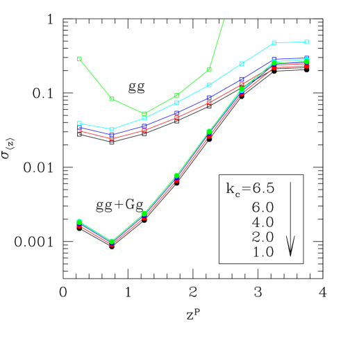
Figure 10: The dependence of self-calibration performance on the shape of galaxy power spectrum. We adopt a toy model of galaxy clustering, characterized as a power law with a break at $k=k_{c}$. The shown value of $k_{c}$ is in unit of $h/$Mpc. The ad-hoc galaxy power spectrum is closer to a power law for larger $k_{c}$. As expected, when the galaxy power spectrum is closer to a power law (with redshift-independent power index), the self-calibration based on galaxy clustering alone degrades and eventually blows up, due to more severe degeneracy between up and down photo-z scatters. On the other hand, the full self-calibration virtually avoids this problem, since it heavily relies on the intrinsic lensing geometry dependence to break this degeneracy.

To investigate this issue, we adopt an ad-hoc model for galaxy clustering, in which the galaxy bias is scale dependent such that 3D galaxy power spectrum (variance) takes the form

$$\Delta_{g}^{2}(k,z)=10^{1.25}k^{1.85}(1+z)^{-2}\ \ when\ \ k<k_{c}\ ,$$ (16)

and $\Delta_{g}^{2}(k,z)=\Delta_{g}^{2}(k_{c},z)$ when $k\geq k_{c}$. If $k_{c}>1h/$Mpc, at $z=0$ and $0.1h/$Mpc $\la k<1h/$Mpc, it is close to the matter power spectrum (variance) $\Delta_{m}^{2}(k,z=0)$ and thus close to the galaxy clustering with $b_{g}=1$. But it shows significant deviation from the matter power spectrum at other $k$ and other redshifts. In the limit that $k_{c}\rightarrow\infty$, this galaxy power spectrum becoms a strict power-law and we expect that the self-calibration based on galaxy clustering alone fails. Numerically, we find that when $k_{c}\ga 7h/$Mpc, the Fisher matrix inversion based on galaxy clustering alone blows up, indicating its failure.

Fig. 10 shows the degradation when increasing $k_{c}$. Despite better galaxy clustering measurement due to stronger clustering strength, the self-calibration accuracy degrades, since the galaxy power spectrum is closer to a strict power-law and the degeneracy between up and down photo-z scatters becomes more severe.

We expect that the full self-calibration is basically free of this problem, since it mainly relies on the lensing geometry dependence to break the degeneracy between up and down scatters—namely, a lens can only lens a galaxy behind it. This is indeed what we find numerically. To demonstrate this point, we assume the galaxy bias with respect to the matter density to be deterministic, thus the 3D matter-galaxy cross correlation power spectrum (variance) is given by

$$\Delta^{2}_{mg}(k,z)=\sqrt{\Delta^{2}_{g}(k,z)\times\Delta^{2}_{m}(k,z)}\ .$$ (17)

This quantity determines the galaxy-galaxy lensing power spectrum. The accuracy of the full self-calibration is shown in Fig. 10. The reconstruction accuracy only degrades slightly even when the galaxy power spectrum is very close to a strict power-law (e.g. $k_{c}=6.5h/$Mpc).

This extreme example confirms our expectation that scale dependence of the galaxy bias is unlikely to alter the major conclusions of this paper, namely the feasibility of our self-calibration technique.

5.2 Dependence on other specifications

The scaling of $p_{i\rightarrow j}$ reconstruction accuracy with fiducial quantities can be roughly understood as follows. The observed density-density correlations $C\propto p^{2}b_{g}^{2}\Delta^{2}_{m}$ and the shear-density correlations $C\propto p^{2}b_{g}\Delta^{2}_{m}$, where $\Delta^{2}_{m}$ is the matter power spectrum (variance). These are the signals. For the noises in the correlation measurements, we have shown that shot noises in shear and galaxy number density measurements are the only relevant ones, which scale as $\gamma_{\rm rms}(f_{\rm sky}\bar{n}_{g}^{2})^{-1/2}$ and $(f_{\rm sky}\bar{n}_{g}^{2})^{-1/2}$ respectively.

Then if relying on galaxy-galaxy lensing measurement alone, the reconstruction error $\sigma_{p}\propto\gamma_{\rm rms}^{1}$. In combination with galaxy-galaxy clustering measurement, the dependence becomes weaker and we expect that $\sigma_{p}\propto\gamma_{\rm rms}^{e}$, where $e\in(0,1)$. If we adopt a fiducial value $\gamma_{\rm rms}=0.24$ instead of $0.2$, the reconstruction accuracy will degrade by a factor of $<20\%$.

For fixed galaxy distribution, matter power spectrum $\Delta^{2}_{m}$, and $p_{i\rightarrow j}$, following similar argument above, we find that

$$\sigma_{p}\propto f_{\rm sky}^{-1/2}\bar{n}_{g}^{-1}b_{g}^{-d}\gamma_{\rm rms}^{e}\ .$$ (18)

Here, the bias dependence $d\in(1,2)$ and, as a reminder, $e\in(0,1)$.

It is interesting to quantify the performance of the self-calibration technique for surveys like CFHTLS and DES. Based on the above scalings, we are able to do an order of magnitude estimation. (1) One of the major differences between these surveys and the fiducial stage IV survey, is the sky coverage. From the $f_{\rm sky}$ dependence alone, for CFHTLS, we expect a factor of 10 larger reconstruction errors, since the sky coverage is a factor of 100 smaller. For DES, we expect the degradation to be a factor of 2. Since the statistical accuracy of these surveys scales exactly the same way with respect to the sky coverage $f_{\rm sky}$, the self-calibration technique works equally fine for these surveys, from this viewpoint. (2) Another difference is that the number density of source galaxies in CFHTLS and DES is likely a factor of 2 smaller. This results in another factor of 2 degradation in the reconstruction accuracy. Since the lensing measurement at $\ell<2000$ is not completely shot noise dominated, the statistical accuracy has weaker dependence on $\bar{n}_{g}$. From this viewpoint, the self-calibration technique works better for surveys with higher galaxy number density.

We caution that the above estimation neglects many complexities. For example, CFHTLS, DES and Pan-STARRS are shallower than the fiducial survey and thus the galaxy number densities at high redshift in these surveys are likely much smaller, while the galaxy number densities at low redshift are comparable. This implies that the $p_{i\rightarrow j}$ reconstruction in these surveys at high-z is more affected that at low-z. Furthermore, the above estimation neglects the difference in the photo-z error, which is likely considerably worse for CFHTLS and DES. It will definitely affect the reconstruction. However, as we discussed in §2.4, the detection threshold of contamination rate ($p_{i\rightarrow j}$) is mainly determined by the ratio of noise and signal of corresponding true-z bins. In this sense, the self-calibration technique works better for worse photo-z estimation.

For a robust forecast of the performance of our self-calibration technique in each specific survey, we need a detail fiducial model of the galaxy distribution, clustering and photo-z error distribution. Although this task is beyond the scope of this paper, the above estimates imply that the self-calibration technique will be applicable.

6 Discussions

It is possible to further improve the statistical accuracy of the self-calibration technique. For example, so far we treat $C^{Gg}_{i>j}$ and $C^{Gg}_{k>j}$ as independent quantities. Improvement can be made by utilizing their internal connection. Both of them are determined by the same mass-galaxy cross correlation over the same redshift range. For this reason, they are connected by a simple scaling relation (in the absence of intrinsic alignments), as pointed out by Jain & Taylor [17], Zhang et al. [44], Bernstein [4].

In weak lensing cosmology, people often disregard the lensing power spectrum measurement at $\ell>2000$-$3000$, because theoretical prediction at such scale is largely uncertain. However, the shear-shear measurement at such scales contains useful information to improve the photo-z reconstruction as well as shear-ratio information that is useful for cosmology. For example, they allow for better handle over the magnification and size bias induced correlations, mainly in the background density-foreground shear correlation measurement. We could use this information usually disregarded in cosmological applications to improve the photo-z calibration.

So far we only focus on the reconstructed $p_{i\rightarrow j}$. The reconstructed $C^{gg,R}_{ii}$ and $C^{Gg,R}_{i\geq j}$ contain valuable information on cosmology and can be further explored. Since these reconstructed power spectra do not suffer from the problem of the photo-z scatters, they can be utilized for purpose beyond cosmology. For example, the self-calibration of galaxy intrinsic alignment, proposed by Zhang [45], relies on the measurement of $C^{Gg,P}_{ii}$ to infer the GI correlation contaminated the weak lensing measurement. This quantity is contaminated by the photo-z scatters. Since we are now able to quantify the photo-z scatters and $C^{Gg,R}_{ij}$ simultaneously, we are able to quantify and correct for the effect of photo-z scatters in the self-calibration of galaxy intrinsic alignment.

One key issue missing in this paper is to propagate the errors or biases on the reconstructed $p_{i\rightarrow j}$ into errors on cosmology inferred from shear-shear data. This will tell us whether the errors in the self-calibration are small enough to avoid significant biases or inflated errors in a shear-shear cosmology measurement. Although many of the $p$’s are uncertain by more than the $\sim 0.1\%$ that is needed to make the biases negligible [6], there are many correlations between these errors which complicate the estimation. This issue definitely deserves further investigation.

We emphasize that our purely photometric self-calibration technique is complementary to those based on cross correlations between photo-z and spec-z samples [26, 5], which we call cross-calibration. An advantage of cross-calibration is that it can identify a special type of photo-z error, namely when the mean photo-z is a monotonic increasing function of true-z (other than the correct identity function). As explained earlier, the self-calibration technique fails completely for such type of photo-z error. The cross-calibration technique will also likely be more able to infer galaxy distribution bias caused when photo-z outliers have a different $n(z)$ than other galaxies in the same true-z bin. On the other hand, the self-calibration has a number of advantage over the cross correlation. Since the total number of photo-z galaxies is much larger than that of the spec-z sample, it can reach higher statistical accuracy. Since what it measures is the photo-z scatters in the whole survey volume, it avoids possible cosmic variance in the photo-z scatters, which could bias the cross-calibration. And since the spec-z targets may be a very different population from the photo-z galaxies, the cross-correlation method will be more susceptible to biases from varying $b_{g}$ among subpopulations.

The photo-z scatter self-calibration method described here has many attractive aspects: it does not depend on any cosmological priors or on models of the power spectrum; it is unaffected by intrinsic alignments; its errors are determined by shot noise, not sample variance, so that higher source densities are exploited if observed; it remains Gaussian and tractable to high $\ell$; and is not significantly affected by shear measurement errors. And of course it can be conducted with the same imaging data used for the shear-shear correlation measurement without degrading the shear-shear information content. The Fisher analysis suggests that photo-z outlier rates can be determined with statistical errors of 0.01–1% for bins at $z\leq 2$. It will be necessary to correct data for lensing magnification bias, and in principle this can be done with little statistical penalty, but the magnification bias factor $g$ must be determined to sufficient accuracy. The biggest issue is “galaxy distribution bias,” whereby photo-z outlier galaxies might have different $n(z)$ or bias $b_{g}$ than the non-outlying galaxies in the same true-z bin. We find that the effective bias of galaxies must vary by $<O(0.1)$ in order to avoid systematic errors in scattering rates that exceed the expected statistical errors. This is an area deserving of more detailed attention.

In this paper, we have presented a concept study of the proposed self-calibration. For the idealized survey of stage IV survey specifications, we have shown that it can in principle reconstruct the photo-z error distribution to useful precision. More robust forecast shall include all extra sources of error, as listed in §3 and §4, more realistic fiducial model (§5), and possibly more uncertainties, into account.

7 Acknowledgment

We thank Hu Zhan, Sarah Bridle and Jun Pan for many useful discussions and the anonymous referee for many useful suggestions. PJZ thanks the hospitality of the UPenn physics and astronomy department and the Aspen center for physics, where part of the work was done. PJZ thanks the support of the one-hundred talents program of the Chinese academy of science, the national science foundation of China (grant No. 10533030, 10543004, 10821302 & 10973027), the CAS grant KJCX3-SYW-N2 and the 973 program grant No. 2007CB815401. GMB acknowledges support from grant AST-0607667 from the National Science Foundation and Department of Energy grant DOE-DE-FG02-95ER40893.

Appendix A The likelihood analysis and the Fisher matrix layout

We work on the likelihood of the band angular power spectra to quantify the self-calibration error. As explained in §2, the error estimation here is distinctly different from that in the routine exercises of cosmological parameter constraints and the only relevant noise term is the shot noise. This makes the error estimation much simpler. Here we recast this argument in a more formal way.

The data we have are a set of measured power spectra contaminated by shot noise, $C^{D}=C^{P}+\delta C^{S}$. Here, the superscript “D” denotes the data. $\delta C^{S}$ is the fluctuation in shot noise. $C^{P}$ are the power spectra in photo-z bins, which are related to $C^{R}$ by a set of $p_{i\rightarrow j}$ through Eq. 3 & 5. We want to know the likelihood function $P(p_{i\rightarrow j}|C^{D})$. Since the distribution of $C^{D}$ is completely determined by $p_{i\rightarrow j}$ and $C^{R}$ (given the shot noise distribution), Bayes’ theorem states

$$P(p_{i\rightarrow j},C^{R}|C^{D})\propto P(C^{D}|p_{i\rightarrow j},C^{R})P(p_{i\rightarrow j},C^{R})=P(C^{D}|p_{i\rightarrow j},C^{R})P(p_{i\rightarrow j})P(C^{R})\ .$$ (19)

We then have

$$P(p_{i\rightarrow j}|C^{D})=\int P(p_{i\rightarrow j},C^{R}|C^{D})dC^{R}\propto\int P(C^{D}|p_{i\rightarrow j},C^{R})P(p_{i\rightarrow j})P(C^{R})dC^{R}\ .$$ (20)

For $p_{i\rightarrow j}$, we only exert the condition $\sum_{i}p_{i\rightarrow j}=1$. Since we do not take any cosmological prior, we set the prior $P(C^{R})=1$. Then Eq. 20 means to marginalize over all possible value of $C^{R}$. This is what we have done in the paper. Notice that $P(C^{D}|p_{i\rightarrow j},C^{R})$ is completely determined by the shot noise distribution, given $C^{R}$ and $p_{i\rightarrow j}$, the parameters that we want to fit. That is the reason that we state that only shot noise shows up in the error analysis. And, since we do not have real data, we have to arbitrarily choose $C^{D}$, which could differ from the cosmic mean, due to the existence of cosmic variance. This freedom is where the cosmic variance shows up. In the paper, we follow the common choice and set $C^{D}=\langle C^{R}\rangle$, the ensemble average. But this is just a representative case of the real data. Namely, $C^{D}$ can be any other value in the range allowed by the cosmic variance and the shot noise, as discussed in one of the footnotes in §2.4.

In Eq. 20, we can take stronger prior on $C^{R}$. In principle, if we know the cosmology, we can write down the full PDF of $C^{R}$. In reality, we do not know exactly the cosmology and we do not know exactly the PDF in the non-linear, non-Gaussian regime. Nevertheless, these priors will improve the reconstruction accuracy of $p_{i\rightarrow j}$. However, as we show in the paper, the systematical error induced by galaxy distribution bias may have already been the dominant error source, improvement over statistical error is not necessary at the current moment.

Since the fluctuations are induced by the shot noise, the central limit theorem implies that we can approximate the probability distribution of the power spectra $P(C^{D}|p_{i\rightarrow j},C^{R})$ as Gaussian, as long as there are sufficiently large number of independent $\vec{\ell}$ modes in each multipole $\ell$ bin ($\ell\Delta{\ell}f_{\rm sky}\gg 1$). Since we only use those modes with $\ell>100$ and $\Delta l\gg 1$, the probability distribution of the power spectra should be Gaussian for $f_{\rm sky}\ga 0.01$. Furthermore, the covariance matrix is diagonal, namely, different power spectrum measurements are uncorrelated, since the associated shot noises are uncorrelated. The covariance matrix between the power spectra $C^{(\alpha),P}_{i_{1}j_{1}}$ and $C^{(\beta),P}_{i_{2}j_{2}}$, with $(\alpha),(\beta)=gg,Gg$, is

$$C^{(\alpha),(\beta)}_{i_{1}j_{1};i_{2}j_{2}}=\left[\sigma_{i_{1}j_{1}}^{(\alpha)}\right]^{2}\delta_{(\alpha)(\beta)}\delta_{i_{1}i_{2}}\delta_{j_{1}j_{2}}\ ,$$ (21)

with

$$(\sigma^{gg}_{ij})^{2}=\frac{\left[4\pi f_{\rm sky}/N_{i}\right]\left[4\pi f_{\rm sky}/N_{j}\right]}{2\ell\Delta\ell f_{\rm sky}}(1+\delta_{ij})\ ,\ (\sigma^{Gg}_{ij})^{2}=\frac{\left[4\pi f_{\rm sky}\gamma^{2}_{\rm rms}/N_{i}\right]\left[4\pi f_{\rm sky}/N_{j}\right]}{2\ell\Delta\ell f_{\rm sky}}\ .$$ (22)

The logarithm of the likelihood function is

$$\ln L=-\frac{1}{2}\sum_{\ell}\left[\sum_{i\leq j}\left(\sigma^{gg}_{ij}(\ell)\right)^{-2}\left(C^{gg,D}_{ij}(\ell)-C^{gg,P}_{ij}(\ell)\right)^{2}+\sum\left(\sigma^{Gg}_{ij}(\ell)\right)^{-2}\left(C^{Gg,D}_{ij}(\ell)-C^{Gg,P}_{ij}(\ell)\right)^{2}\right]+{\rm const}.\ \ .$$ (23)

Here, $C^{gg,P}_{ij}$ and $C^{Gg,P}_{ij}$ are the model prediction, given by Eq. 3 & 5. If the model is unbiased, we can set $C^{gg,D}=C^{gg,P}$ and $C^{Gg,D}=C^{Gg,P}$ when evaluating the Fisher matrix $F_{ij}\equiv\partial^{2}\ln L/\partial\lambda_{i}\partial\lambda_{j}$. We then have

$${\bf F}_{km}=\sum_{\ell}\left[\sum_{i\leq j}\left(\sigma^{gg}_{ij}(\ell)\right)^{-2}\frac{\partial C^{gg,P}_{ij}(\ell)}{\partial\lambda_{k}}\frac{\partial C^{gg,P}_{ij}(\ell)}{\partial\lambda_{m}}+\sum_{ij}\left(\sigma^{Gg}_{ij}(\ell)\right)^{-2}\frac{\partial C^{Gg,P}_{ij}(\ell)}{\partial\lambda_{k}}\frac{\partial C^{Gg,P}_{ij}(\ell)}{\partial\lambda_{m}}\right]\ .$$ (24)

$C^{gg,P}_{ij}$ and $C^{gg,P}_{ji}$ are equivalent, so we only need to sum up pairs with $i\leq j$ for the galaxy-galaxy correlation. On the other hand, for the lensing-galaxy cross correlation, we should sum up all pairs (in this case, $ij$ and $ji$ pairs are asymmetric). The unknown parameters to be determined are $\lambda=(p_{\mu\rightarrow\nu},C^{Gg,R}_{ij}(\ell_{1}),C^{gg,R}_{kk}(\ell_{1})\ldots)$, with $\mu\neq\nu$, $i\geq j$ and $\mu,\nu,i,j,k=1,\ldots$. Here, $\ell_{1,2\ldots}$ denote the multipole $\ell$ bins. The Fisher matrix can be decomposed as follows,

$${\bf F}=\bordermatrix{&&\cr&{\bf A}&{\bf B}\cr&{\bf C}&{\bf D}\cr}=\bordermatrix{&&&&\cr&\sum_{\ell}{\bf A_{\ell}}&{\bf B}_{\ell_{1}}&\ldots&{\bf B}_{\ell_{n}}\cr&{\bf C}_{\ell_{1}}&{\bf D}_{\ell_{1}}&\ldots&0\cr&\vdots&\vdots&\ddots&\vdots\cr&{\bf C}_{\ell_{n}}&0&\ldots&{\bf D}_{\ell_{n}}\cr}\ .$$ (25)

Here, ${\bf A}\equiv{\bf F}_{p_{\mu_{1}\nu_{1}}p_{\mu_{2}\nu_{2}}}$. It is the sum of ${\bf A}_{\ell}$, the contribution from each $\ell$ bin. ${\bf B}\equiv{\bf F}_{p_{\mu_{1}\nu_{1}}C_{\mu_{2}\nu_{2}}}$ and ${\bf C}={\bf B}^{T}$. ${\bf B}$ can be decomposed as ${\bf B}=({\bf B}_{\ell_{1}},{\bf B}_{\ell_{2}},\ldots)$, where ${\bf B}_{\ell}$ is the contribution from each $\ell$ bin. ${\bf D}={\bf F}_{C_{\mu_{1}\nu_{1}}C_{\mu_{2}\nu_{2}}}$. Since different $\ell$ bins do not correlate, ${\bf D}$ is block diagonal and denote each block element as ${\bf D}_{\ell}$. The exact definitions of ${\bf A}_{\ell}$, ${\bf B}_{\ell}$, ${\bf C}_{\ell}$ and ${\bf D}_{\ell}$ can be found by comparing Eq. 23 and 25. The dimension of ${\bf A}$ and ${\bf A}_{l}$ is $N_{z}(N_{z}-1)\times N_{z}(N_{z}-1)$. That of ${\bf B}_{\ell}$ is $N_{z}(N_{z}-1)\times N_{z}(N_{z}+3)/2$ and that of ${\bf D}_{\ell}$ is N${}_{z}(N_{z}+3)/2\times N_{z}(N_{z}+3)/2$. The inverse of ${\bf F}$ is

$${\bf F}^{-1}=\bordermatrix{&&\cr&\left({\bf A}-{\bf B}{\bf D}^{-1}{\bf C}\right)^{-1}&-\left({\bf A}-{\bf B}{\bf D}^{-1}{\bf C}\right)^{-1}{\bf B}{\bf D}^{-1}\cr&-{\bf D}^{-1}{\bf C}\left({\bf A}-{\bf B}{\bf D}^{-1}{\bf C}\right)^{-1}&{\bf D}^{-1}+{\bf D}^{-1}{\bf C}\left({\bf A}-{\bf B}{\bf D}^{-1}{\bf C}\right)^{-1}{\bf B}{\bf D}^{-1}\cr}\ .$$ (26)

For convenience, we define

$${\bf A}^{\rm reduced}\equiv{\bf A}-{\bf B}{\bf D}^{-1}{\bf C}=\sum_{\ell}\left[{\bf A}_{\ell}-{\bf B}_{\ell}{\bf D}^{-1}_{\ell}{\bf C}_{\ell}\right]\equiv\sum_{\ell}{\bf A}^{\rm reduced}_{\ell}\ .$$ (27)

The second expression holds because ${\bf D}$ is block diagonal. The reduced matrix ${\bf A}^{\rm reduced}$ determines the reconstruction accuracy of $p_{i\rightarrow j}$. The last expression simply means that, since $\ell$ bins are uncorrelated, we are able to sum over the contribution from each of them and improve the reconstruction accuracy. We know that constrains on the photo-z scatters mainly come from $C^{Gg,P}_{i<j}$ and $C^{gg,P}_{i\neq j}$. So we can further decompose ${\bf A}_{\ell}={\bf A}^{\rm min}_{\ell}+\Delta{\bf A}_{\ell}$, where ${\bf A}^{\rm min}_{\ell}$ is the contribution from $C^{Gg,P}_{i<j}$ and $C^{gg,P}_{i\neq j}$ and $\Delta{\bf A}_{\ell}$ is the contribution from $C^{Gg,P}_{i\geq j}$ and $C^{gg,P}_{i=j}$. For clarity, we provide the expression of $\Delta{\bf A}_{\ell}$,

$$\Delta{\bf A}_{\ell,km}=\sum_{i=j}\left(\sigma^{gg}_{ij}(\ell)\right)^{-2}\frac{\partial C^{gg,P}_{ij}(\ell)}{\partial\lambda_{k}}\frac{\partial C^{gg,P}_{ij}(\ell)}{\partial\lambda_{m}}+\sum_{i\geq j}\left(\sigma^{Gg}_{ij}(\ell)\right)^{-2}\frac{\partial C^{Gg,P}_{ij}(\ell)}{\partial\lambda_{k}}\frac{\partial C^{Gg,P}_{ij}(\ell)}{\partial\lambda_{m}}\ .$$ (28)

Here, $\lambda_{k},\lambda_{m}\in p_{\mu\nu}$.

In the limit $p_{\mu\neq\nu}\rightarrow 0$ (equivalently $p_{\mu\rightarrow\nu}\rightarrow\delta_{\mu\nu}$), we have $\Delta{\bf A}_{\ell}\rightarrow{\bf B}_{\ell}{\bf D}^{-1}_{\ell}{\bf C}_{\ell}$. The proof is as follows. since $p_{i\rightarrow j}=\delta_{ij}$, ${\bf D}_{\ell}$ is diagonal, with the diagonal elements ${\bf D}_{C^{Gg}_{\mu_{1}\nu_{1}};C^{Gg}_{\mu_{1}\nu_{1}}}=(\sigma^{Gg}_{\mu_{1}\nu_{1}})^{-2}$ and ${\bf D}_{C^{gg}_{\mu_{1}\mu_{1}};C^{gg}_{\mu_{1}\mu_{1}}}=(\sigma^{gg}_{\mu_{1}\mu_{1}})^{-2}$. We then have

$${\bf B}_{\ell}{\bf D}^{-1}_{\ell}{\bf C}_{\ell}=\sum_{i=j}\left(\sigma^{gg}_{ij}(\ell)\right)^{-2}\frac{\partial C^{gg,P}_{ij}(\ell)}{\partial\lambda_{k}}\frac{\partial C^{gg,P}_{ij}(\ell)}{\partial\lambda_{m}}+\sum_{i\geq j}\left(\sigma^{Gg}_{ij}(\ell)\right)^{-2}\frac{\partial C^{Gg,P}_{ij}(\ell)}{\partial\lambda_{k}}\frac{\partial C^{Gg,P}_{ij}(\ell)}{\partial\lambda_{m}}=\Delta{\bf A}_{\ell}\ .$$ (29)

Thus under the limit that $p_{i\neq j}\rightarrow 0$, ${\bf A}^{\rm reduced}={\bf A}^{\rm min}$ and the the error matrix of $p$ is $[{\bf A}^{\rm min}]^{-1}$. This result has a clear physical meaning. We know that the measurements $C^{gg,P}_{i=j}$ and $C^{Gg,P}_{i\geq j}$ are most responsible for determining $C^{gg,R}_{i=j}$ and $C^{Gg,R}_{i\geq j}$ and the measurements $C^{gg,P}_{i\neq j}$ and $C^{Gg,P}_{i<j}$ are most responsible to determine $p$. Under the limit $p_{i\neq j}\rightarrow 0$, we are able to have a clear separation of the two sets of measurements.

We caution that with the presence of photo-z scatters, this is no longer the case. Numerically, we find that the presence of photo-z scatters make the statistical error in $p$ reconstruction, larger than the above limiting case.

We now derive the detailed expression of all the matrices. A useful relation in this exercise is that $\partial p_{k\rightarrow i}/\partial p_{\mu\rightarrow\nu}=\delta_{i\nu}(\delta_{k\mu}-\delta_{k\nu})$. The last term shows up because $p_{i\rightarrow i}=1-\sum_{k\neq i}p_{k\rightarrow i}$ and only $p_{\mu\neq\nu}$ are independent variables. We then have

$$\frac{\partial C_{ij}^{(\alpha),P}}{\partial p_{\mu\rightarrow\nu}}=\delta_{i\nu}\sum_{m}\left(C_{\mu m}^{(\alpha),R}-C_{\nu m}^{(\alpha),R}\right)p_{m\rightarrow j}+\delta_{j\nu}\sum_{k}\left(C_{k\mu}^{(\alpha),R}-C_{k\nu}^{(\alpha),R}\right)p_{k\rightarrow i}\equiv\delta_{i\nu}A_{\mu\nu j}^{(\alpha)}+\delta_{j\nu}B_{\mu\nu i}^{(\alpha)}\ .$$ (30)

Clearly, we have $A_{\mu\nu i}^{gg}=B_{\mu\nu i}^{gg}$. But there is no such relation for the G-g terms. Finally we have

$${\bf A}^{\rm min}_{\ell,p_{\mu_{1}\rightarrow\nu_{1}},p_{\mu_{2}\rightarrow\nu_{2}}} = \sum^{(\alpha)}\left[\left(\sigma_{\nu_{1}\nu_{2}}^{(\alpha)}\right)^{-2}A_{\mu_{1}\nu_{1}\nu_{2}}^{(\alpha)}B_{\mu_{2}\nu_{2}\nu_{1}}^{(\alpha)}H(\nu_{2}-\nu_{1})+\left(\sigma_{\nu_{2}\nu_{1}}^{(\alpha)}\right)^{-2}B_{\mu_{1}\nu_{1}\nu_{2}}^{(\alpha)}A_{\mu_{2}\nu_{2}\nu_{1}}^{(\alpha)}H(\nu_{1}-\nu_{2})\right.$$ (31)

$$+ \left.\sum_{j>\nu_{1}}\left(\sigma_{\nu_{1}j}^{(\alpha)}\right)^{-2}A_{\mu_{1}\nu_{1}j}^{(\alpha)}A_{\mu_{2}\nu_{2}j}^{(\alpha)}\delta_{\nu_{1}\nu_{2}}+\sum_{i<\nu_{1}}\left(\sigma_{i\nu_{1}}^{(\alpha)}\right)^{-2}B_{\mu_{1}\nu_{1}i}^{(\alpha)}B_{\mu_{2}\nu_{2}i}^{(\alpha)}\delta_{\nu_{1}\nu_{2}}\right]\ ,$$

$$\Delta{\bf A}_{\ell,p_{\mu_{1}\rightarrow\nu_{1}},p_{\mu_{2}\rightarrow\nu_{2}}} = \delta_{\nu_{1}\nu_{2}}\left(\sigma_{\nu_{1}\nu_{1}}^{(gg)}\right)^{-2}\times(A_{\mu_{1}\nu_{1}\nu_{1}}^{(gg)}+B_{\mu_{1}\nu_{1}\nu_{1}}^{(gg)})(A_{\mu_{2}\nu_{1}\nu_{1}}^{(gg)}+B_{\mu_{2}\nu_{1}\nu_{1}}^{(gg)})$$ (32)

$$+ \left(\sigma_{\nu_{1}\nu_{2}}^{(Gg)}\right)^{-2}A_{\mu_{1}\nu_{1}\nu_{2}}^{(Gg)}B_{\mu_{2}\nu_{2}\nu_{1}}^{(Gg)}H(\nu_{1}-\nu_{2})+\left(\sigma_{\nu_{2}\nu_{1}}^{(Gg)}\right)^{-2}B_{\mu_{1}\nu_{1}\nu_{2}}^{(Gg)}A_{\mu_{2}\nu_{2}\nu_{1}}^{(Gg)}H(\nu_{2}-\nu_{1})$$

$$+ \sum_{j\leq\nu_{1}}\left(\sigma_{\nu_{1}j}^{(Gg)}\right)^{-2}A_{\mu_{1}\nu_{1}j}^{(Gg)}A_{\mu_{2}\nu_{2}j}^{(Gg)}\delta_{\nu_{1}\nu_{2}}+\sum_{i\geq\nu_{1}}\left(\sigma_{i\nu_{1}}^{(Gg)}\right)^{-2}B_{\mu_{1}\nu_{1}i}^{(Gg)}B_{\mu_{2}\nu_{2}i}^{(Gg)}\delta_{\nu_{1}\nu_{2}}\ ,$$

$${\bf B}_{\ell,p_{\mu_{1}\rightarrow\nu_{1}},C^{Gg}_{\mu_{2}\nu_{2}}}=\sum(\sigma_{\nu_{1}j}^{Gg})^{-2}A_{\mu_{1}\nu_{1}j}p_{\mu_{2}\rightarrow\nu_{1}}p_{\nu_{2}\rightarrow j}+\sum_{i\neq\nu_{1}}(\sigma_{i\nu_{1}}^{Gg})^{-2}B_{\mu_{1}\nu_{1}i}p_{\mu_{2}\rightarrow i}p_{\nu_{2}\rightarrow\nu_{1}}\ ,$$ (33)

$${\bf B}_{\ell,p_{\mu_{1}\rightarrow\nu_{1}},C^{gg}_{\mu_{2}\nu_{2}}}=\sum_{j\geq\nu_{1}}(\sigma_{\nu_{1}j}^{gg})^{-2}A_{\mu_{1}\nu_{1}j}p_{\mu_{2}\rightarrow\nu_{1}}p_{\nu_{2}\rightarrow j}+\sum(\sigma_{i\nu_{1}}^{gg})^{-2}B_{\mu_{1}\nu_{1}i}p_{\mu_{2}\rightarrow i}p_{\nu_{2}\rightarrow\nu_{1}}\ ,$$ (34)

$${\bf D}_{\ell,C^{Gg}_{\mu_{1}\nu_{1}},C^{Gg}_{\mu_{2}\nu_{2}}}=\sum(\sigma_{ij}^{Gg})^{-2}p_{\mu_{1}\rightarrow i}p_{\nu_{1}\rightarrow j}p_{\mu_{2}\rightarrow i}p_{\nu_{2}\rightarrow j}\ ,$$ (35)

and

$${\bf D}_{\ell,C^{gg}_{\mu_{1}\nu_{1}},C^{gg}_{\mu_{2}\nu_{2}}}=\sum_{i\leq j}(\sigma_{ij}^{gg})^{-2}p_{\mu_{1}\rightarrow i}p_{\nu_{1}\rightarrow j}p_{\mu_{2}\rightarrow i}p_{\nu_{2}\rightarrow j}\ ,$$ (36)

Here, $H(x)$ is the Heaviside step function, whose value is $1$ when $x$ is positive, otherwise zero. In the above equations, all the power spectra at the right hand sides are evaluated at the corresponding $\ell$.

We now only need to invert the matrix ${\bf D}_{\ell}$ and ${\bf A}^{\rm reduced}$. This is a much easier job than the inversion of the full Fisher matrix ${\bf F}$. More than that, it improves the numerical stability and accuracy of the inversion, which we can check at each step according to Eq. 26 & 27. Numerically, we do not find any numerical instability or singularity for all the configurations that we have tested. The reconstruction accuracy of $p$ is solely determined by ${\bf A}^{\rm reduced}$ and the results are shown in Fig. 3.

Alternative to this detailed description of the photo-z errors, we can evaluate a single convenient number, the density weighted true redshift of the $i$-th photo-z bin. It is defined as

$$\langle z_{i}\rangle=\frac{\int_{0}^{\infty}zn_{i}(z)dz}{N_{i}}=\sum_{j}p_{j\rightarrow i}\frac{\int_{j}zn_{i}(z)dz}{\int_{j}n_{i}(z)dz}\ .$$ (37)

It is not trivial to robustly evaluate $\langle z_{i}\rangle$. The special type of photo-z error, in which the photo-z is a monotonic increasing function of the true-z, discussed in §2, is one of the problems. However, even if such error does not exist, there is still another difficulty. We can measure $p_{j\rightarrow i}$ robustly. However, it only tells us $\int_{j}n_{i}(z)=p_{j\rightarrow i}N_{i}$. Without proper parameterization, we can not derive $n_{i}$ and thus can not robustly evaluate $\langle z_{i}\rangle$. In reality, for those stage IV lensing surveys, the function $n_{i}(z)$ should be sufficiently smooth. This implies that we can interpolate $p_{j\rightarrow i}$ to model $n_{i}(z)$. The simulation data that we used does not have sufficient amount of galaxies allowing us to do this exercise. Instead, we will try two approximations to evaluate $\langle z_{i}\rangle$.

One possibility is the following approximation

$$\langle z_{i}\rangle=\sum_{j}p_{j\rightarrow i}\langle z^{P}_{j}\rangle=\langle z^{P}_{i}\rangle+\sum_{j}(\langle z^{P}_{j}\rangle-\langle z^{P}_{i}\rangle)p_{j\rightarrow i}\ ,$$ (38)

where $\langle z^{P}_{i}\rangle$ is the density weighted average photo-z of the $i$-th photo-z bin. The other possibility is to replace $\langle z^{P}_{i}\rangle$ by the middle-point of this redshift bin. Through our simulation data, we can check the accuracy of the above two approximations. We find that the first approximation is often better. The statistical error in $\langle z_{i}\rangle$, due to statistical errors in $p_{i\rightarrow j}$ is then

$$\sigma^{2}_{i} \simeq \sum_{jk}\left(\langle z^{P}_{j}\rangle-\langle z^{P}_{i}\rangle)(\langle z^{P}_{k}\rangle-\langle z^{P}_{i}\rangle\right)\langle\delta p_{j\rightarrow i}\delta p_{j\rightarrow i}\rangle=\sum_{jk}(\langle z^{P}_{j}\rangle-\langle z^{P}_{i}\rangle)(\langle z^{P}_{k}\rangle-\langle z^{P}_{i}\rangle){\bf F}^{-1}_{p_{j\rightarrow i}p_{k\rightarrow i}}\ .$$ (39)

By far we have assumed that $p_{i\rightarrow j}$ can be any real value. But of course, $0\leq p_{i\rightarrow j}\leq 1$. This condition can be straightforwardly enforced by $p\rightarrow(\tanh(x)+1)/2$, where $x$ can be any real value. Furthermore, there are conditions that $C^{gg,R}_{ii}>0$, which can be automatically satisfied by the transformation $C^{gg,R}\rightarrow\exp(y)$, where $y$ can be any real value. Given the small errors of stage IV lensing projects, these extra conditions are not likely able to improve the reconstruction accuracy significantly. However, for stage 3 projects like CFHTLS, these conditions should be explicitly enforced to improve the reconstruction accuracy.

Appendix B The induced bias

The self-calibration is based on the validity of Eq. 3 and 5. Systematic deviations from these equation then induce systematic errors in $p_{i\rightarrow j}$. Here we outline the calculation of such bias. The bias in reconstructed $\lambda$ is $\delta\lambda\equiv\lambda^{F}-\lambda^{T}$. $\lambda^{F}$ is determined by requiring $\partial\ln L/\partial\lambda|_{\lambda^{F}}=0$. Taylor expanding this equation at $\lambda^{T}$ and keeping terms up to $O(\delta\lambda)$, we obtain a set of linear equations on $\Delta\lambda$ and its solution

$${\bf F}_{ij}\delta\lambda_{j}={\bf J}_{i}\ \ ;\ \ \delta\lambda_{i}={\bf F}^{-1}_{ij}{\bf J}_{j}\ ,$$ (40)

where

$${\bf J}_{m}=\sum_{i\leq j}(\sigma^{gg}_{ij})^{-2}\delta C^{gg}_{ij}\frac{\partial C_{ij}^{gg,P}}{\partial\lambda_{m}}+\sum(\sigma^{Gg}_{ij})^{-2}\delta C^{Gg}_{ij}\frac{\partial C_{ij}^{Gg,P}}{\partial\lambda_{m}}\ .$$ (41)

Here, $\delta C^{\alpha}_{ij}\equiv C_{ij}^{\alpha,D}-C_{ij}^{\alpha,P}(\lambda^{T})$ is the model bias in the corresponding power spectrum. For example, for the galaxy distribution bias, we have $\delta C^{gg}_{ij}=\sum_{k}p_{k\rightarrow i}p_{k\rightarrow j}(\tilde{b}_{k\rightarrow i}\tilde{b}_{k\rightarrow j}-1)C^{gg}_{kk}$ and $\delta C^{Gg}_{ij}=\sum_{k>m}p_{k\rightarrow i}p_{m\rightarrow j}(\tilde{b}_{m\rightarrow j}-1)C^{Gg}_{km}$. Noticing that, since $\delta\lambda\propto\delta C$, we have also neglected terms $O(\delta C\times\delta\lambda)$ when deriving this equation. All differentials in Eq. 41 are evaluated at $\lambda^{T}$. This result agrees with that in Huterer & Takada [14], Huterer et al. [15]. The related matrices are calculated from the following expressions,

$${\bf J}_{p_{\mu\rightarrow\nu}}=\sum_{j\geq\nu}(\sigma^{gg}_{\nu j})^{-2}\delta C^{gg}_{\nu j}A^{gg}_{\mu\nu j}+\sum_{i\leq\nu}(\sigma^{gg}_{i\nu})^{-2}\delta C^{gg}_{i\nu}B^{gg}_{\mu\nu i}+\sum(\sigma^{Gg}_{\nu j})^{-2}\delta C^{Gg}_{\nu j}A^{Gg}_{\mu\nu j}+\sum(\sigma^{Gg}_{i\nu})^{-2}\delta C^{Gg}_{i\nu}B^{Gg}_{\mu\nu i}\ ,$$ (42)

$${\bf J}_{C^{Gg}_{\mu\nu}}=\sum(\sigma^{Gg}_{ij})^{-2}\delta C^{Gg}_{ij}p_{\mu\rightarrow i}p_{\nu\rightarrow j}\ ,$$ (43)

and

$${\bf J}_{C^{gg}_{\mu\nu}}=\sum_{i\leq j}(\sigma^{gg}_{ij})^{-2}\delta C^{gg}_{ij}p_{\mu\rightarrow i}p_{\nu\rightarrow j}\ .$$ (44)

The induced bias in individual $p_{i\rightarrow j}$ is shown in Fig. 7. The induced bias in the mean redshift is

$$\delta z_{i}\simeq\sum_{j}(\langle z^{P}_{j}\rangle-\langle z^{P}_{i}\rangle)\delta p_{j\rightarrow i}\ .$$ (45)

The numerical results are shown in Fig. 8 & 9.

References

- Albrecht et al. [2006] Report of Dark Energy Task Force. Andreas Albrecht, et al. arXiv:astro-ph/0609591
- Amara & Réfrégier [2008] Amara, A., & Réfrégier, A. 2008, MNRAS, 391, 228
- Bacon et al. [2000] Bacon, D. J., Refregier, A. R., & Ellis, R. S. 2000, MNRAS, 318, 625
- Bernstein [2006] Bernstein, G. 2006, ApJ, 637, 598
- Bernstein [2009] Bernstein, G. M. 2009, ApJ, 695, 652
- Bernstein & Huterer [2009] Bernstein, G., & Huterer, D. 2009, arXiv:0902.2782
- Fu et al. [2008] Fu, L., et al. 2008, AAP, 479, 9
- Heitmann et al. [2005] Heitmann, K., Ricker, P. M., Warren, M. S., & Habib, S. 2005, ApJS, 160, 28
- Heitmann et al. [2008] Heitmann, K., White, M., Wagner, C., Habib, S., & Higdon, D. 2008, arXiv:0812.1052
- Heitmann et al. [2009] Heitmann, K., Higdon, D., White, M., Habib, S., Williams, B. J., & Wagner, C. 2009, arXiv:0902.0429
- Heymans et al. [2006] Heymans, C., et al. 2006, MNRAS, 368, 1323
- Hirata et al. [2004] Hirata, C. M., et al. 2004, MNRAS, 353, 529 PRD, 70, 063526
- Hirata et al. [2007] Hirata, C. M., Mandelbaum, R., Ishak, M., Seljak, U., Nichol, R., Pimbblet, K. A., Ross, N. P., & Wake, D. 2007, MNRAS, 381, 1197
- Huterer & Takada [2005] Huterer, D., & Takada, M. 2005, Astroparticle Physics, 23, 369
- Huterer et al. [2006] Huterer, D., Takada, M., Bernstein, G., & Jain, B. 2006, MNRAS, 366, 101
- Jain [2002] Jain, B. 2002, ApJ, 580, L3
- Jain & Taylor [2003] Jain, B., & Taylor, A. 2003, Physical Review Letters, 91, 141302
- Jain & Zhang [2008] Jain, B., & Zhang, P. 2008, PRD, 78, 063503
- Jing et al. [2006] Jing, Y. P., Zhang, P., Lin, W. P., Gao, L., & Springel, V. 2006, ApJ, 640, L119
- Joachimi & Bridle [2009] Joachimi, B., & Bridle, S. L. 2009, arXiv:0911.2454
- Jouvel et al. [2009] Jouvel, S., et al. 2009, arXiv:0902.0625
- Kaiser et al. [2000] Kaiser, N., Wilson, G., & Luppino, G. A. 2000, arXiv:astro-ph/0003338
- Ma, Hu, & Huterer [2006] Ma, Z., Hu, W., & Huterer, D. 2006, ApJ, 636, 21
- Mandelbaum et al. [2006] Mandelbaum, R., Hirata, C. M., Ishak, M., Seljak, U., & Brinkmann, J. 2006, MNRAS, 367, 611
- Massey et al. [2007] Massey, R., et al. 2007, MNRAS, 376, 13
- Newman [2008] Newman, J. A. 2008, ApJ, 684, 88
- Okumura et al. [2009] Okumura, T., Jing, Y. P., & Li, C. 2009, ApJ, 694, 214
- Okumura & Jing [2009] Okumura, T., & Jing, Y. P. 2009, ApJ, 694, L83
- Pen [2004] Pen, U.-L. 2004, MNRAS, 350, 1445
- Rudd et al. [2008] Rudd, D. H., Zentner, A. R., & Kravtsov, A. V. 2008, ApJ, 672, 19
- Schmidt et al. [2009] Schmidt, F., Rozo, E., Dodelson, S., Hui, L., & Sheldon, E. 2009, arXiv:0904.4702
- Schneider et al. [2006] Schneider, M., Knox, L., Zhan, H., & Connolly, A. 2006, ApJ, 651, 14
- Seljak & Zaldarriaga [1996] Seljak, U., & Zaldarriaga, M. 1996, ApJ, 469, 437
- Seljak [2009] Seljak, U. 2009, Physical Review Letters, 102, 021302
- Smith et al. [2003] Smith, R. E., et al. 2003, MNRAS, 341, 1311
- Van Waerbeke et al. [2000] Van Waerbeke, L., et al. 2000, AAP, 358, 30
- White [2004] White, M. 2004, Astroparticle Physics, 22, 211
- Wittman et al. [2000] Wittman, D. M., Tyson, J. A., Kirkman, D., Dell’Antonio, I., & Bernstein, G. 2000, Nature, 405, 143
- Zehavi et al. [2004] Zehavi, I., et al. 2004, ApJ, 608, 16
- Zhan & Knox [2004] Zhan, H., & Knox, L. 2004, ApJ, 616, L75
- Zhan & Knox [2006] Zhan, H., & Knox, L. 2006, ApJ, 644, 663
- Zhan [2006] Zhan, H. 2006, Journal of Cosmology and Astro-Particle Physics, 8, 8
- Zhan & Knox [2006] Zhan, H., & Knox, L. 2006, arXiv:astro-ph/0611159
- Zhang et al. [2005] Zhang, J., Hui, L., & Stebbins, A. 2005, ApJ, 635, 806
- Zhang [2008] Zhang, P. 2008, arXiv:0811.0613