The Supermassive Black Hole and Dark Matter Halo of NGC 4649 (M60)

Abstract

We apply the axisymmetric orbit superposition modeling to estimate the mass of the supermassive black hole and dark matter halo profile of NGC 4649. We have included data sets from the Hubble Space Telescope, stellar, and globular cluster observations. Our modeling gives $M_{\bullet}=(4.5\pm 1.0)\times 10^{9}M_{\odot}$ and ${\rm M/L}_{V\rm,\;obs}=8.7\pm 1.0$ (or ${\rm M/L}_{V}=8.0\pm 0.9$ after foreground Galactic extinction is corrected). We confirm the presence of a dark matter halo, but the stellar mass dominates inside the effective radius. The parameters of the dark halo are less constrained due to the sparse globular cluster data at large radii. We find that in NGC 4649 the dynamical mass profile from our modeling is consistently larger than that derived from the X-ray data over most of the radial range by roughly 60% to 80%. It implies that either some forms of non-thermal pressure need to be included, the assumed hydrostatic equilibrium may not be a good approximation in the X-ray modelings of NGC 4649, or our assumptions used in the dynamical models are biased. Our new $M_{\bullet}$ is about two times larger than the previous published value; the earlier model did not adequately sample the orbits required to match the large tangential anisotropy in the galaxy center. If we assume that there is no dark matter, the results on the black hole mass and ${\rm M/L}_{V\rm,\;obs}$ do not change significantly, which we attribute to the inclusion of HST spectra, the sparse globular cluster kinematics, and a diffuse dark matter halo. Without the HST data, the significance of the black hole detection is greatly reduced.

1. Introduction

Most nearby galaxies harbor supermassive black holes at their centers. Correlations between black hole (BH) mass and host galaxy properties (Magorrian et al., 1998; Gebhardt et al., 2000; Ferrarese & Merritt, 2000; Häring & Rix, 2004) have been used extensively in theoretical models in order to understand growth of the black hole and galaxy (e.g., Hopkins et al., 2008). The latest work from Hopkins et al. suggest that a main role of a black hole is to halt star formation in the galaxy when the black hole is large enough, thereby causing the dichotomy in colors (e.g., Bell, 2008). While there is still an active debate as to the relative role of AGN feedback versus star formation feedback, there is a consensus that physical mechanisms for black hole growth are very important for understanding mass growth in galaxies. A concern is that the black hole correlations may have significant systematic biases, both from kinematics with poor spatial resolution and models that do not adequately include the full mass profile (see discussion in Gültekin et al. 2009).

Dynamical modeling of galaxies using orbit superposition offers one of the best estimates on the black hole mass (e.g., Rix et al., 1997; van der Marel et al., 1998; Cretton et al., 1999; Gebhardt et al., 2000, 2003; Valluri et al., 2004; Thomas et al., 2004, 2005; Siopis et al., 2009). Assuming axisymmetry, these models do not limit the form of the allowed velocity anisotropies. Thus, the stellar orbital structure resulting from the dynamical modeling provides a unique window on the mass growth process in the massive systems, as long as the model assumptions are valid.

A particular systematic bias is shown in Gebhardt & Thomas (2009) where they find that the black hole mass can be underestimated in the most massive galaxies if the dark halo is not included. They find a degeneracy between the dark halo and black hole mass, since without the dark halo the stellar mass-to-light ratio is overestimated which subsequently decreases the required contribution of the black hole to constrain the central kinematics. In M87, Gebhardt & Thomas (2009) find that the black hole mass goes from $2.5\times 10^{9}$ to $6.4\times 10^{9}~{}M_{\odot}$ by simply running models including a dark halo. Furthermore, the uncertainties do not overlap, implying a large systematic effect. In M87, however, this degeneracy is strong since the black hole is not well resolved by the kinematic data. For galaxies with well spatially-resolved kinematics, we do not expect the degeneracy to be as significant.

In addition to studying the black hole mass, there is a strong need to study the shapes of dark matter profiles. There is still little consensus for those measured in individual galaxies (e.g., PNe from Romanowsky et al. 2003, stellar light from Forestell & Gebhardt 2008, X-rays from Gastaldello et al. 2007; Churazov et al. 2008; Humphrey et al. 2008, 2009, and globular clusters from Bridges et al. 2006; Hwang et al. 2008). The impressive work using gravitational lensing to measure the average dark matter profiles (e.g., Mandelbaum et al. 2006a, b) has been able to reach out to nearly 1 Mpc. However, these results need to be compared to measurements based on individual galaxies. It is important to understand the galaxy-to-galaxy scatter in the profiles and whether there are environmental effects.

This paper is part of an extensive campaign to measure both the black hole mass and the dark matter profile simultaneously, to examine the possible bias of the dark matter profile on the black hole mass estimate for galaxies with various profiles, and to compare with the gravitational potentials derived with other independent techniques such as the X-rays and weak lensing studies. Initially, we focus on the more massive galaxies, but it will be important to extend future analysis over a large mass range. Gebhardt & Thomas (2009) report results for M87, the most massive nearby elliptical, and in this paper we focus on NGC 4649. Both galaxies are giant ellipticals with a central surface brightness “core”.

In this paper we present the axisymmetric orbit superposition models for NGC 4649 (M60), combining data from the Hubble Space Telescope (HST), stellar, and globular cluster observations. NGC 4649 is a giant elliptical with low surface brightness located in a subclump to the east of the main Virgo concentration (Forbes et al., 2004). NGC 4649 has been studied extensively for its total mass profile in recent X-ray modelings (e.g., Humphrey et al., 2006; Gastaldello et al., 2007; Humphrey et al., 2008), and globular cluster studies (e.g., Bridges et al., 2006). The goals of our study are to place NGC 4649’s black hole mass estimate on a more solid footing, to infer the properties of its dark matter halo, and more importantly to offer an independent cross-check using different dynamical tracers to the previous studies on NGC 4649.

We assume a distance to NGC 4649 of 15.7 Mpc. At this distance, 1$\arcsec$ corresponds to 76 pc.

2. Data

Figure 1.— The $V$-band volume luminosity density profile for stars. This comes from the deprojection of the surface brightness profile presented in Kormendy et al. (2009).

The input data of NGC 4649 (surface brightness profile and kinematics) have all been previously published, and we rely on that data for the models presented here. We use the stellar surface brightness profile compiled by Kormendy et al. (2009) from a variety of sources, including HST imaging as presented in Lauer et al. (2005). All data from Kormendy et al. (2009) have been transformed to $V$-band, and extend to about 700″. We deproject the surface brightness using Abel’s formula as in Gebhardt et al. (1996). The volume luminosity density we derived is plotted in Figure 1. The effective radius $R_{e}$ of NGC 4649 is about $90\arcsec$ by fitting a de Vaucouleurs profile to its surface brightness profiles.

The stellar kinematics are the same as used in Gebhardt et al. (2003), and are presented in Pinkney et al. (2003). These data include long-slit observations on HST STIS and three position angles from ground-based observations (see Pinkney et al. 2003 for details). There are no new stellar kinematic data presented in this paper. The HST spectra extend to 0.8″, and the ground-based stellar data extend to 70″. The dynamical modeling code uses the line-of-sight velocity distribution (LOSVD), which are the same as used in Gebhardt et al. (2003).

In order to extend to yet further radii, we also include data from globular cluster (GC) velocities. The GC kinematics come from Hwang et al. (2008), which combine kinematic data from Bridges et al. (2006) and Lee et al. (2008). There are 121 clusters with velocities over a radial range from 32–533″. However, we only use the velocities that are beyond 200″, since inside that radius the clusters with velocities are spread over too many model bins to add any significant information compared to the stellar kinematics. A further complication with using GCs in the central parts is that their number density profile is not well known there. Outside of 200″, there are 61 clusters with velocities, and the average radius of these clusters is 319″ (Hwang et al., 2008). Rotation in the GC system at radii beyond 200″ is reported in Hwang et al. (2008); however, Bridges et al. (2006) argue for little to no rotation at radii around 200″. We therefore explore models where we include the rotation directly (by fitting a velocity profile on the major axis at 319″ with a rotation amplitude and velocity dispersion as reported by Hwang et al. 2008) and where we use the second moment of the GC velocities only (by fitting one velocity profile, centered on zero velocity, to the GC velocities in the full annulus). The results are nearly identical. In this paper, we only present results from using the second moment. Our analysis of the Hwang et al. data implies a second moment of 267($\pm 25$) km/s, which is consistent with the analysis of Bridges et al. (2006). Since the modeling code uses LOSVDs directly, we must transform the moments into LOSVDs, which we do using Monte Carlo realizations of the values and uncertainties (as discussed in Gebhardt et al. 2003).

The dynamical models require the number density profile of the GCs (since we use clusters as a tracer population). Hwang et al. (2008) present number density profiles of the GCs. We use their equation 5 for the combined sample as the deprojected number density profile. Comparing this profile to the stellar luminosity density shows that beyond 150″, the two profiles have the same slope. Inside that radius, the GC number density profile flattens more compared to the stars. Since we do not use any clusters inside of 200″, we cadopt the same number density profile for the clusters as we do for the stars.

Figure 2.— $\chi^{2}$ versus ${\rm M/L}_{V\rm,\;obs}$, black hole mass $M_{\bullet}$, the halo scale velocity $V_{\rm c}$, and the halo core radius $r_{\rm c}$. Each point represents a possible model for the logarithmic halo (only models with $\Delta\chi^{2}\lesssim 25$ over the minimum are shown in order to highlight the $1\sigma$ uncertainty). The solid line along the bottom ridge represents the marginalized $\chi^{2}$ values which we use to determine the best fit and uncertainties. The horizontal line marks the 68% confidence limit ($\Delta\chi^{2}=1.0$).

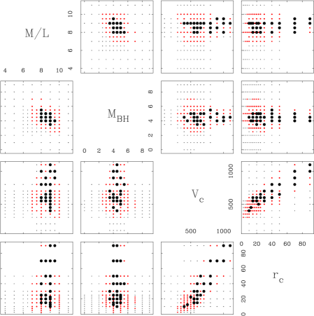
Figure 3.— Plots of the $V$-band ${\rm M/L}_{V\rm,\;obs}$, black hole mass $M_{\bullet}$ (in units of $10^{9}M_{\odot}$), the scale velocity $V_{\rm c}$ of the logarithmic halo in ${\rm km/s}$, and the core radius $r_{\rm c}$ of the logarithmic halo in kpc against each other to show possible degeneracies. The small grey points represent the locations of all the models. The large black points are the locations of those models that are within the 68% confidence limit ($\Delta\chi^{2}=1.0$) after marginalizing over the other possible parameters. The red points are those that are within the 95% confidence band. The strong correlation between $V_{\rm c}$ and $r_{\rm c}$ is apparent.

3. Dynamical Models

The orbit superposition models we use are based on the idea invented by Schwarzschild (1979), and are described in detail in Gebhardt et al. (2000, 2003); Thomas et al. (2004, 2005); Siopis et al. (2009). The models have been tested extensively to recover both the black hole mass and the dark matter halo without significant bias for axisymmetric systems.

We first determine the luminosity density from the surface brightness profile as described in §2. Although we have constructed models using different inclinations, we generally assume that the galaxy is edge-on and adopt the minor-to-major axial ratio of 0.9. Next we compute the gravitation field from the 3-D light distribution assuming that the mass consists of a black hole with mass $M_{\bullet}$, and stars with a constant ${\rm M/L}_{V\rm,\;obs}$ ratio independent of position, and a dark matter halo (now parametrized with only logarithmic and NFW profiles).

Next our orbit-based model is implemented in two steps: constructing the orbit library and fitting the full LOSVD (as opposed to using only the second velocity moments) with the orbit library. We measure the LOSVD in radius and angle relative to the symmetry axis of the galaxy, and in velocity. We use 24 radial, 5 angular, and 15 velocity bins. The radial range of the dynamical models extend to 1000″. We calculate the galaxy potential and force on a grid that is 5 times finer than the grid used in the data comparison. We carefully choose the initial positions of the orbits to generate a sufficiently dense sampling of $E$, $L_{z}$, and $I_{3}$ (Thomas et al., 2004). This ensures a reliable representation of the full phase space. Generally we have at least $30,000$ orbits when both the black hole and dark matter halo are included.

We then choose the orbital weights so the superposition of orbits match the light distribution and LOSVDs of the galaxy as well as possible. The orbital weights are derived from the maximization of the objective function $\hat{S}=S-\alpha\chi^{2}$ where $S$ is an approximation to the usual Boltzmann entropy and $\chi^{2}$ is the sum of squared residuals to the data. The smoothing parameter $\alpha$ controls the influence of the entropy $S$ on the orbital weights. We cannot specify the optimal value of $\alpha$ in advance. In practice we start with a very small $\alpha$ and gradually increase it until the improvement in $\chi^{2}$ is less than a given percentage in a single iteration. We have verified that our results are not sensitive to the choice of the smoothing parameter $\alpha$.

We ran nearly 16,000 different models to estimate the black hole mass and the dark matter halo parameters. Each model has a distinct set of orbit library, and takes about 1.5 hours on the supercomputer lonestar of the Texas Advanced Computing Center.

4. Results

4.1. Models including a dark matter halo

In our canonical set of models, the mass distribution $\rho$ of NGC 4649 consists of a central black hole, stellar mass density, and a dark matter halo:

$$\rho=M_{\bullet}\delta(r)+\Upsilon\nu+\rho_{\rm DM}$$

where $\Upsilon={\rm M/L}_{V\rm,\;obs}$ is the mass-to-light ratio of the stars (a position-independent constant), and $\nu$ is the observed $V$-band stellar luminosity density. ${\rm M/L}_{V\rm,\;obs}$ needs to be corrected with the foreground Galactic extinction in order to compare with that derived from stellar population models. A popular foreground Galactic extinction value $A_{V}=0.088$ (Schlegel et al., 1998) could be adopted; it gives the extinction-corrected ${\rm M/L}_{V}={\rm M/L}_{V\rm,\;obs}/1.084$.

We describe the dark matter halo with a logarithmic profile, whose density is given as

$$\rho_{\rm DM}=\frac{V_{\rm c}^{2}}{4\pi G}\frac{3r_{\rm c}^{2}+r^{2}}{(r_{\rm c}^{2}+r^{2})^{2}}$$

and potential as

$$\Phi=\frac{1}{2}V_{\rm c}^{2}\ln(1+\frac{r^{2}}{r_{\rm c}^{2}}).$$

Gebhardt & Thomas (2009) found that realistic NFW models that fit the globular cluster kinematics are not centrally concentrated enough to dominate the mass in the inner regions; the enclosed mass profile they get with NFW models are very similar to those obtained with logarithmic halos. Thus, whether we parameterize with an NFW or a logarithmic halo will have little influence on the black hole mass estimate, particularly true for NGC 4649 where HST spectra exist. We focus on a logarithmic halo in this study.

The kinematics include all data sets from the HST, stellar, and globular cluster observations (§2). We use the $\chi^{2}$ distribution from all possible models to determine the four best-fit parameters (${\rm M/L}_{V\rm,\;obs}$, $M_{\bullet}$, $V_{\rm c}$, $r_{\rm c}$), and the associated uncertainties. We start with a uniform but sparse grid in the 4-D parameter space, then sample the smallest $\chi^{2}$ region with a finer grid. As we will see from the figures below, the $\chi^{2}$ minimum and the contours of NGC 4649 are quite regular, so our sampling procedure should be adequate to cover the parameter space near the best-fit values. The uncertainties in the parameters are determined from the change in the marginalized $\chi^{2}$ as we vary one of the variables; $\Delta\chi^{2}=1$ above the minimum represents the 68% confidence band or 1$\sigma$ uncertainty. We use the middle of the 68% confidence range as the best-fit value and half of that range as the uncertainty.

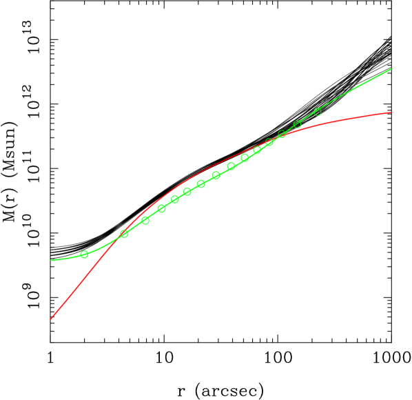
Figure 4.— The mass profile for NGC 4649. The black lines represent the models that are within the 68% confidence band of the best fit (as in Figure 3). The green line is our representation of the X-ray derived enclosed mass profile (the green circles, as in Gastaldello et al. 2007; Humphrey et al. 2008). The parameters for the green line are $M_{\bullet}=3.5\times 10^{9}\;M_{\odot}$, ${\rm M/L}_{V\rm,\;obs}=5.0$, $V_{\rm c}=410{\rm km/s}$, and $r_{\rm c}=10{\rm kpc}$. The red line is the average contribution from the stars, where we integrate the light profile in Figure 1 then times 8.7 (the best-fit ${\rm M/L}_{V\rm,\;obs}$). Clearly the total mass profile obtained from our modeling is consistently larger than that from X-rays over most of the radial range.

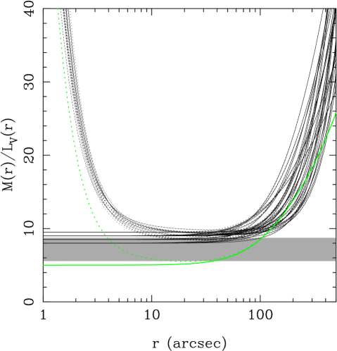
Figure 5.— The integrated ${\rm M/L}_{V\rm,\;obs}$ as a function of radius. The black dotted lines represent the models that are within the 68% confidence band of the best-fit potentials (black lines in Figure 4). The black solid lines are the same models but excluding the contribution from the black hole. The green solid and dotted are our best representation of the X-ray potential without and with a black hole. The shaded horizontal band is the range of possible ${\rm M/L}_{V\rm,\;obs}$ (after applying the foreground Galactic extinction of $A_{V}=0.088$) from stellar population models (Maraston, 1998, 2005), depending on what form of IMF is assumed.

Figure 2 presents $\chi^{2}$ as a function of ${\rm M/L}_{V\rm,\;obs}$, the black hole mass $M_{\bullet}$, the halo scale velocity $V_{\rm c}$, and the halo core radius $r_{\rm c}$, including all values for the other three parameters. Each point represents a possible model, but we show only models near the $\chi^{2}$ minimum to highlight the $1\sigma$ uncertainty. The solid line along the bottom ridge represents the marginalized $\chi^{2}$ values which we use to determine the best fit and uncertainties. Given the number of LOSVDs, the velocity binning used in the modeling, and that the LOSVD bins are correlated (as discussed in Gebhardt et al. 2003), the reduced $\chi^{2}$ is around 0.4, which is typical with orbit-based models.

From Figure 2, we find the black hole mass $M_{\bullet}=(4.5\pm 1.0)\times 10^{9}M_{\odot}$ and the stellar ${\rm M/L}_{V\rm,\;obs}=8.7\pm 1.0$ (or ${\rm M/L}_{V}=8.0\pm 0.9$ after foreground Galactic extinction is corrected with $A_{V}=0.088$). The scale velocity $V_{\rm c}$ and the core radius $r_{\rm c}$ of the logarithmic halo are not well constrained. As we will discuss later, halo parameters are degenerate with each other, and their exact values have little effect on the shape of the dark matter profile in the region of interest.

In order to find the possible correlations and degeneracies in the four parameters, Figure 3 plots ${\rm M/L}_{V\rm,\;obs}$, $M_{\bullet}$, $V_{\rm c}$ and $r_{\rm c}$ against each other. The small grey points represent the locations of all the models. The large black and red points highlight those models that are within the 68% ($\Delta\chi^{2}=1.0$) and the 95% ($\Delta\chi^{2}=4.0$) confidence bands, respectively, after marginalizing over the other possible parameters. The strong correlation between $V_{\rm c}$ and $r_{\rm c}$ is apparent. This is because the dynamical models only fit for the enclosed mass and we do not have enough kinematics at large radii; we cannot distinguish dark halos with a large $V_{\rm c}$ and a large $r_{\rm c}$ from the one with a small $V_{\rm c}$ and an accordingly fine-tuned small $r_{\rm c}$. By the same token, the degeneracy between ${\rm M/L}_{V\rm,\;obs}$ and $M_{\bullet}$ (apparent in the the 95% confidence band) is expected; the decreasing/increasing contribution from the stars can be made up by having a larger/smaller black hole mass, to certain extent. For NGC 4649, the degeneracy between ${\rm M/L}_{V\rm,\;obs}$ and $M_{\bullet}$ is relatively weak because the inclusion of HST data makes the uncertainties in $M_{\bullet}$ much smaller, unlike in M87’s case (Gebhardt & Thomas, 2009). HST spectra provide good spatial sampling inside of the region where the black hole dominates over stars. We do not find obvious degeneracies among other parameters.

The radial profile of the enclosed mass in NGC 4649 is shown in Figure 4. The black lines represent the models that are within the 68% confidence band of the best fit (large black points in Figure 3). The red line stands for the stellar contribution alone using the best-fit ${\rm M/L}_{V\rm,\;obs}$ of 8.7. The stellar component clearly dominates the mass profile from $10\arcsec$ to $100\arcsec$. At the effective radius $R_{e}$ ($\sim$ 90″), the best-fit stellar mass accounts for about 75% of the total enclosed mass. Within $10\arcsec$ the $4.5\times 10^{9}M_{\odot}$ black hole is dominant, while outside $100\arcsec$ the dark matter halo prevails. Compared with NGC 4649, the best-fit dark halo of M87 is much more dominant (Gebhardt & Thomas, 2009). This also shows that ellipticals with comparable luminosities can have quite different distributions of dark matter relative to stars.

Figure 5 presents the integrated mass-to-light ratio ${\rm M/L}_{V\rm,\;obs}$ as a function of radius. The black dotted lines are the total ${\rm M/L}_{V\rm,\;obs}$ of the models that are within the 68% confidence band of the best-fit potentials (black lines in Figure 4). The black solid lines are the same models but excluding the contribution from the black hole. Consistent with Figure 4, Figure 5 shows that the increase of the total ${\rm M/L}_{V\rm,\;obs}$ at small radius is dictated by the black hole, and the increase at large radius is due to the dark matter halo. In the intermediate radial range, from $10\arcsec$ to $100\arcsec$, the ${\rm M/L}_{V\rm,\;obs}$ is a constant that stellar contribution dominates.

Figure 6.— $\chi^{2}$ distribution when a logarithmic halo with $V_{\rm c}=410{\rm km/s}$ and $r_{\rm c}=10{\rm kpc}$, which best matches the results of X-ray modeling (the green line in Figure 4), is imposed in the modeling. (a): $\chi^{2}$ as a function of black hole mass $M_{\bullet}$, including all values in ${\rm M/L}_{V\rm,\;obs}$. Each point represents a model, however, not all models that we ran are shown in order to highlight the $1\sigma$ uncertainty. The solid line along the bottom ridge represents the marginalized $\chi^{2}$ values which we use to determine the best fit and uncertainties. The horizontal line marks the 68% confidence limit ($\Delta\chi^{2}=1.0$). (b): as in (a) but for $\chi^{2}$ as a function of $V$-band ${\rm M/L}_{V\rm,\;obs}$, including all values in $M_{\bullet}$. (c): 2-D plot of $\chi^{2}$ as a function of black hole mass and ${\rm M/L}_{V\rm,\;obs}$. The points represent models that we ran. As in Gebhardt et al. (2002), the contours were determined by a 2-D smoothing spline interpolated from the these models and represent $\Delta\chi^{2}$ of 1.0, 2.71, 4.0 and 6.63 (corresponding to 68%, 90%, 95%, and 99% for 1 degree of freedom).

Figure 7.— The radial profile of $\Delta\chi^{2}$, which is the difference in the radius-cumulated $\chi^{2}$ between the best-fit model ($M_{\bullet}=4.5\times 10^{9}\;M_{\odot}$, ${\rm M/L}_{V\rm,\;obs}=9.0$, $V_{\rm c}=550{\rm km/s}$, and $r_{\rm c}=15{\rm kpc}$) and the model that best matches the X-ray derived potential ($M_{\bullet}=3.5\times 10^{9}\;M_{\odot}$, ${\rm M/L}_{V\rm,\;obs}=5.0$, $V_{\rm c}=410{\rm km/s}$, and $r_{\rm c}=10{\rm kpc}$).

The shaded band in Figure 5 shows the wide range of possible ${\rm M/L}_{V\rm,\;obs}$ from stellar population models derived as below. We first adopt the age ($\approx$ 12 Gyr) and metallicity $[Z/H]\approx 0.25$ for NGC 4649 from Trager et al. (2000). With the age and metallicity, we then interpolate for the stellar ${\rm M/L}_{V}$ from tables produced by the evolutionary population synthesis models (Maraston, 1998, 2005). If the Salpeter IMF (0.1 to 100 $M_{\odot}$) is assumed, then we get the interpolated stellar ${\rm M/L}_{V}=8.06$ as the upper bound of the shaded area. If the Kroupa IMF (0.1 to 100 $M_{\odot}$) is used instead, then we obtain the interpolated ${\rm M/L}_{V}=5.13$ as the lower bound. In order to compare with our uncorrected ${\rm M/L}_{V\rm,\;obs}$ in Figure 5, we have to multiply the ${\rm M/L}_{V}$ from stellar population models by a factor of 1.084 ($A_{V}=0.088$) to mimic the foreground Galactic extinction. From Figure 5 we see that our best fit ${\rm M/L}_{V\rm,\;obs}=8.7\pm 1.0$ agrees best with the stellar population modeling result assuming the Salpeter IMF, but it is also consistent with the range of results assuming different IMFs.

Figure 8.— As in Figure 6, but for the $\chi^{2}$ distribution when no dark halo is included in the modeling. Large radii kinematics are excluded in the models. The absolute values of $\chi^{2}$ in this figure are not comparable to those in Figure 2 and 6, as this figure fits to less kinematic data (75 data points from the one LOSVD for the globular kinematics and 4 LOSVDs for stellar kinematics beyond 40″are excluded).

4.1.1 Comparison with the X-ray results

In Figure 4 we also include the the mass profile inferred from X-ray modelings (Gastaldello et al., 2007; Humphrey et al., 2008), shown as the green circles. They are derived from the traditional approach, i.e., from the smoothed parametric fits to the temperature and density of the X-ray emitting gas assuming hydrostatic equilibrium. The green line in Figure 4 is our best representation of the X-ray derived mass, assuming a logarithmic dark halo. The parameters for the green line are $M_{\bullet}=3.5\times 10^{9}\;M_{\odot}$, ${\rm M/L}_{V\rm,\;obs}=5.0$, $V_{\rm c}=410{\rm km/s}$, and $r_{\rm c}=10{\rm kpc}$. In Figure 5 the green solid and dotted lines are the ${\rm M/L}_{V\rm,\;obs}$ of our best representation of the X-ray potential without and with a black hole, respectively.

The total mass profile obtained from our modeling is consistently larger than that from X-rays over most of the radial range by a factor of about 1.7. Our stellar mass alone is larger than the X-ray derived mass, so the difference cannot be due to the different dark matter halos derived from the two methods. Our best-fit black hole mass is consistent within the 1$\sigma$ error, yet about 35% larger than, of the $M_{\bullet}=3.35\times 10^{9}M_{\odot}$ derived in Humphrey et al. (2008). Detailed discussions on the difference from the X-ray mass profile are in §5.1.

A concern from this work could be that the dark halo parameters are poorly constrained by the globular cluster kinematics, leading to a biased result on the mass profile and potentially on the black hole mass. We therefore include the X-ray data in two different ways to compare with our dynamical models. First, we use the X-rays to determine the large radii mass profile, allowing our dynamical models to determine the stellar M/L and black hole mass. Second, we adopt the full X-ray mass profile as measured by Humphrey et al. (2008) and compare with our best-fit model.

First, to use the large radii mass profile as determined from the X-rays, we run a grid of models assuming the X-ray dark halo potential ($V_{\rm c}=410{\rm km/s}$, and $r_{\rm c}=10{\rm kpc}$), and fit for black hole mass and stellar ${\rm M/L}_{V\rm,\;obs}$. In other words, we fix only the outer part of the green line in Figure 4, and allow the inner mass profile to seek the best fit to the data. The results are shown in the distribution of $\chi^{2}$ as function of $M_{\bullet}$ and ${\rm M/L}_{V\rm,\;obs}$ in Figure 6. We still find very similar $M_{\bullet}$ and ${\rm M/L}_{V\rm,\;obs}$ as in the canonical set of models (§4.1); both the best-fit values and the $1\sigma$ uncertainties of $M_{\bullet}$ and ${\rm M/L}_{V\rm,\;obs}$ in Figure 6 are very similar to those found in Figure 2 and Figure 3.

Second, we run the mass model with the X-ray derived parameters ($M_{\bullet}=3.5\times 10^{9}\;M_{\odot}$, ${\rm M/L}_{V\rm,\;obs}=5.0$, $V_{\rm c}=410{\rm km/s}$, and $r_{\rm c}=10{\rm kpc}$), and find the best fit to the kinematic data. The $\chi^{2}$ of this model is about $98$, which is a much worse fit than our best-fit model ($\chi^{2}\approx 43.5$). So the stellar and globular cluster kinematics are indeed inconsistent with the X-ray derived mass profile. Figure 7 demonstrates how $\Delta\chi^{2}$ changes with radius, where $\Delta\chi^{2}$ is the difference in the radius-cumulated $\chi^{2}$ between the best-fit model in Figure 2 ($M_{\bullet}=4.5\times 10^{9}\;M_{\odot}$, ${\rm M/L}_{V\rm,\;obs}=9.0$, $V_{\rm c}=550{\rm km/s}$, and $r_{\rm c}=15{\rm kpc}$) and the model with the X-ray derived parameters (the green line in Figure 4, $M_{\bullet}=3.5\times 10^{9}\;M_{\odot}$, ${\rm M/L}_{V\rm,\;obs}=5.0$, $V_{\rm c}=410{\rm km/s}$, and $r_{\rm c}=10{\rm kpc}$). The roughly linear increase of $\Delta\chi^{2}$ with radius indicates that data from all radial range contribute equally to the difference in the total $\chi^{2}$. This is another reason why the assumed outer potential from X-rays does not affect the best-fit $M_{\bullet}$ and ${\rm M/L}_{V\rm,\;obs}$.

4.2. Models without a dark matter halo

Gebhardt & Thomas (2009) found that including a proper dark matter halo in the dynamical modeling of M87 can give a factor of two larger black hole mass than excluding one. Here we also do a similar test on how the black hole mass and ${\rm M/L}_{V\rm,\;obs}$ change if we exclude a dark halo in the modeling of NGC 4649 (i.e., the mass distribution is composed of the black hole and the stars only, $\rho=M_{\bullet}\delta(r)+\Upsilon\nu$). Since we know beforehand that the dark halo dominates at very large radii, we intentionally exclude some of the large radii kinematics in order to not be unduly influenced by data that extend well into the dark halo regime. The excluded regions are the one LOSVD for the globular cluster kinematics and the four LOSVDs for the stellar kinematics beyond 40″. We test the effect of including all data, without a dark halo, and find that the resultant stellar ${\rm M/L}_{V\rm,\;obs}$ (a constant independent of radius) is biased to a large value of 11.5, and the minimal $\chi^{2}$ is larger by $\sim 25$. Thus, the large radii kinematics are excluded in the no-halo modeling. Figure 8 presents the $\chi^{2}$ distribution when a dark halo is excluded and the large radii kinematics are excluded. From the marginalized $\chi^{2}$ as a function of $M_{\bullet}$ and ${\rm M/L}_{V\rm,\;obs}$ in Figure 8, we find the black hole mass $M_{\bullet}=(4.3\pm 0.7)\times 10^{9}M_{\odot}$ and the $V$-band stellar ${\rm M/L}_{V\rm,\;obs}=9.0\pm 1.0$. The uncertainties with the no dark halo models are slightly lower than when including a dark halo, and this difference could be due to noise in the $\chi^{2}$ contours in Figure 8. The best-fit black hole mass is quite different from the previously published ones for NGC 4649 in Gebhardt et al. (2003), which are cruder models without a dark halo either; we will discuss this point in detail in §5. Also these values differ from those when a dark matter halo is allowed (§ 4.1) by less than 5%. So in NGC 4649 the inclusion of a proper dark halo does not make as big a difference to the best-fit $M_{\bullet}$ and ${\rm M/L}_{V\rm,\;obs}$ as in the case of M87. The existence of HST data in NGC 4649 certainly helps to alleviate the bias. Also the globular cluster kinematics in NGC 4649 are sparse (only one radial bin), so they do not have as much leverage in the total $\chi^{2}$ as in M87. Furthermore, the dark matter halo of NGC 4649 is not as massive and concentrated as that of M87, so the black hole mass estimate of NGC 4649 is not biased as much by neglecting the dark matter halo.

We further experimented recomputing for the best-fit model using the ground-based spectral data only, excluding the HST spectra. The inclusion of the HST spectra in the modeling undoubtedly improves the significance of the black hole substantially; the $\chi^{2}$ difference between models with the best-fit $M_{\bullet}$ and with zero $M_{\bullet}$ is around 30. The best-fit black hole mass is almost the same, however, the uncertainty in $M_{\bullet}$ becomes much larger when the HST spectra are excluded. This experiment emphasizes the need for the HST spectra to improve the error in the determination of $M_{\bullet}$.

4.3. Velocity Dispersion Tensor

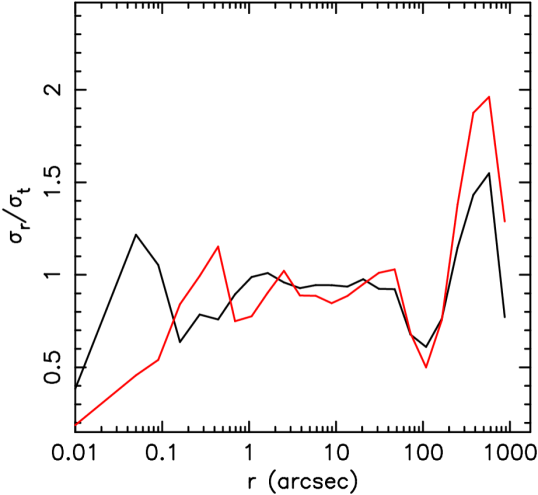
Figure 9.— Shape of the velocity dispersion tensor as a function of radius for the best-fit model. The black line is along the major axis, and the red line is near the minor axis.

Figure 10.— Ratios of the velocity dispersions $\sigma_{r}$/$\sigma_{\theta}$ (top) and $\sigma_{\phi}$/$\sigma_{\theta}$ (bottom) as a function of radius near the equatorial plane for the best-fit model.

We also examine the internal orbital structures by studying the shape of the velocity dispersion tensor. In our work the tangential dispersion is defined as $\sigma_{t}=\sqrt{\sigma_{\phi}^{2}+\sigma_{\theta}^{2}}$, where $\sigma_{\phi}$ includes contributions from both random and ordered motions, i.e., it is the second moment of the azimuthal velocity relative to the systemic velocity instead of to the mean rotation velocity. An non-rotating isotropic model gives $\sigma_{r}$/$\sigma_{t}=1$. Figure 9 shows the internal dispersion ratio $\sigma_{r}$/$\sigma_{t}$ along the major and minor axes for our best fit model ($M_{\bullet}=4.5\times 10^{9}\;M_{\odot}$, ${\rm M/L}_{V\rm,\;obs}=9.0$, $V_{\rm c}=550{\rm km/s}$, and $r_{\rm c}=15{\rm kpc}$). Over most of the radial range, the model is very isotropic. It is strongly tangentially biased near the center, and more radially biased at large radii. Gebhardt et al. (2003) discussed the possibility that the amount of the tangential anisotropy at large radii may be overestimated when the dark matter halo is excluded. The current result shows the orbits are clearly more radially dominated at $r>100\arcsec$ when the dark matter starts to dominate.

We also want to inspect if the distribution function of NGC 4649 truly depends on three integrals of motion or only two: energy $E$ and the $z$-component of the angular momentum $L_{z}$. We know that in a two-integral model, $f=f(E,L_{z})=f(v_{R}^{2}/2+v_{\phi}^{2}/2+v_{z}^{2}/2+\Phi(R,z),Rv_{\phi})$, $\sigma_{R}$ must be equal to $\sigma_{z}$. One way to test whether a two-integral model is sufficient is by comparing $\sigma_{r}$ and $\sigma_{\theta}$ on the equatorial plane where $\sigma_{R}=\sigma_{r}|_{\phi=0}$ and $\sigma_{z}=\sigma_{\theta}|_{\phi=0}$ (Figure 10). The radial variation of $\sigma_{r}/\sigma_{\theta}$ in Figure 10 demonstrates that the best-fit model is inconsistent with having only two integrals of motion, despite that the radially-averaged $\sigma_{r}/\sigma_{\theta}$ is close to one. Thus, our three-integral model is needed to best fit the data. We also show the $\sigma_{\phi}/\sigma_{\theta}$ ratio in the bottom panel of Figure 10. We can see that near the black hole the tangential dispersion is dominated by the azimuthal $\phi$ motion, whereas the $\theta$ and $\phi$ dispersions are similar at most of radii. Such detailed information on the shape of velocity dispersion tensor could be potential constraints on the formation processes of the supermassive black holes.

5. Discussions

5.1. Estimates of the mass profile

From §4.1.1 we see that the total mass profile from our modeling is consistently larger than that from X-rays over most of the radial range by a factor of about 1.7. Also the slopes of the two mass profiles inside the effective radius are quite similar. If our orbit-based modeling results are confirmed in other independent studies, then it may suggest that the X-ray derived mass is systematically lower. There are several possible reasons why the X-ray modeling could underestimate the true mass profile.

X-ray modelings generally assume that the X-ray emitting hot gas is in hydrostatic equilibrium. Diehl & Statler (2007) argue that the X-ray gas may not be in good hydrostatic equilibrium because they found no correlation between X-ray and optical ellipticities in the inner region where stellar mass dominates over dark matter and a shallow correlation should be expected. If the hot gas is not in hydrostatic equilibrium, the inflow of gas can make the X-ray derived mass smaller than the true value (Pellegrini & Ciotti, 2006; Johnson et al., 2009).

Even if the hydrostatic equilibrium holds reasonably well for the X-ray emitting gas, the existence of non-thermal pressure components, but omitted in the X-ray modeling, can still make the X-ray derived mass estimate less than the true value. For example, possible forms of non-thermal pressure support include magnetic field, cosmic rays, and microturbulence (e.g. Brighenti & Mathews, 1997; Churazov et al., 2008; Johnson et al., 2009). Also, since the hot gas in ellipticals comes mainly from the stellar mass loss, infall or mergers, the gas could carry significant amount of angular momentum. The gas can settle into rotationally supported systems as it flows in and spins up. The spherically-determined X-ray mass may again be an underestimate since the rotation is ignored.

However, Brighenti et al. (2009) study NGC 4649 and conclude that turbulant motion in the X-ray gas is not strong enough to bias the derived potential. Our dynamical results are in disagreement with the X-ray derived potential, possibly suggesting that other non-thermal pressures are present. While it is still unclear what combination of systematics contribute to the difference in the mass estimates of the X-ray and orbit-based methods, it is imperative to extend our orbit-based modeling to a larger sample of galaxies that have been analyzed with X-rays, and to examine if the difference between the two methods is general.

5.2. Black Hole Mass

Figure 11.— The modeled and observed LOSVDs at $R=0.18\arcsec$ on the major axis. The y-axis represents the relative projected light for this spatial bin. The data (Pinkney et al., 2003) are shown by the solid dots and their 68% confidence bands (the velocity bins at the edge have a large uncertainty because the original LOSVD extractions from Pinkney et al. 2003 do not extend that far in velocity space). The solid line is the LOSVD from the best-fit model in this paper, and the dashed line is the LOSVD from the best-fit model in Gebhardt et al. (2003). The current model is a significantly improved fit due to the inclusion of the highest angular momentum orbits (i.e., nearly circular orbits) that can match better the flat-topped LOSVD.

The black hole mass reported here is $4.5(\pm 1.0)\times 10^{9}\;M_{\odot}$. Using nearly the same input data, Gebhardt et al. (2003) report a black hole mass of $2.0(\pm 0.5)\times 10^{9}\;M_{\odot}$ (note the reported black hole mass of Gebhardt et al. 2003 has two changes applied to it: first, we decrease the reported mass by 7% for the different distances, and second, we apply a 9% increase in the mass due to a numerical error in the previous calculation as reported in Siopis et al. 2009). While this is only a 1.5-$\sigma$ difference, since we are using the same data, we should get the same result. Thus, any difference must be in the modeling code changes, the input assumptions (e.g., dark halo mass) or a combination. We find that the difference is due to a more complete orbit sampling, discussed below, but we have also checked a variety of other possibilities.

Comparing Figure 8 (no dark halo) with Figure 2 (including a dark halo) shows that there is little difference in the black hole mass when including a dark halo. This is expected since the black hole’s effect on the kinematics is well resolved with the HST kinematics. Other effects, such as the radial range used in the modeling (in the present paper we must extend the galaxy model out to larger radii to include the dark halo), appear to have an insignificant effect as well.

The main modifications used for this study is to increase the orbit library substantially and to sample the phase space differently. For this study, we ran two sets of models, one with 30,000 orbits and one with 13,000 orbits. The results are nearly identical in terms of $\Delta\chi^{2}$ (which is what we use to determine the values and uncertainties), however the minimum $\chi^{2}$ is lower by about 30. Gebhardt et al. (2003) use 7000 orbits, with a $\chi^{2}$ that is larger by 80. Given that we do not see a difference in the current models using different orbit numbers, we are confident that orbit number is not a concern for NGC 4649.

We do, however, find that the change in orbit sampling is the the main factor causing difference in the black hole mass of NGC 4649. The difference in orbit sampling is presented in Thomas et al. (2004), where we now use a sampling based on the density in the meridional plane whereas the previous version (used in Gebhardt et al. 2003) relied on sampling along the zero-velocity curve. In particular, the new sampling covers more completely the phase space occupied by the highest angular momentum orbits for a given energy, like near-circular orbits and shell orbits.

Core galaxies appear to have significant tangential orbital anisotropy in their centers (Gebhardt et al., 2003). Thus, if the orbital coverage poorly sampled important regions of phase space occupied by tangential orbits, this may bias the best-fit model. Indeed, the orbital anisotropy is strongly biased towards tangential motion in the central regions (Section 4.3), much more so than in the original orbit-models of Gebhardt et al. (2003). In Figure 11 we exemplify the comparison of LOSVDs from the old and new orbit sampling, and the observed LOSVD. In the figure the $HST$ observed LOSVD at $R=0.18\arcsec$ on the major axis is quite flat-topped. The modeled LOSVD in the current best-fit model (solid curve) is able to fit the data very well, whereas the best-fit model in Gebhardt et al. (2003) (dashed curve) has trouble matching the profile. The poor fit from the previous model is due to the lack of nearly circular orbits.

Increasing the amount of tangential anisotropy causes the projected dispersion to drop in the central regions; thus, in order to match the observed projected velocity dispersion, the black hole mass has to be increased to compensate. This concern needs to be tested on other galaxies, specifically core galaxies. We note that the work of Siopis et al. (2009) compare black hole masses from analytic models using the same orbital sampling presented here. They find no bias in the black hole masses, but the central density of their galaxy (NGC 4258) is cuspy instead of cored. Galaxies with such a large core as NGC 4649 and large tangential orbital bias should be further studied.

With $M_{\bullet}=4.5\times 10^{9}M_{\odot}$ and the effective stellar velocity dispersion $\sigma_{e}=385\;{\rm km/s}$, NGC 4649’s position is above the latest $M_{\bullet}-\sigma_{e}$ relation (Gültekin et al., 2009) by about 0.33 dex, but still within the intrinsic scatter of the relation. Increasing the largest black hole masses by a factor of 2—NGC 4649 in this paper and M87 in Gebhardt & Thomas (2009)—will have important consequences for understanding the upper mass end (as in Lauer et al. 2007) and comparison with masses as estimated for quasars. There has been a long standing problem as to why some quasars have black hole mass estimates approaching $10^{10}~{}M_{\odot}$, whereas none have ever been measured that high even though the volumes surveyed should be large to see these; a factor of 2 to 3 increase appears to resolve this issue. Furthermore, an underestimate of the black hole mass seriously effects the physical correlations, used extensively to quantify the role of black holes on galaxy evolution (e.g., Hopkins et al. 2008), the amount of deviation from a simple $M_{\bullet}-\sigma_{*}$ power-law relation (Wyithe, 2006), and the number density of the largest black holes (Lauer et al., 2007; Bernardi et al., 2007).

5.3. Main uncertainties

The uncertainties presented in this paper are statistical uncertainties from the $\chi^{2}$ analysis. In order to translate a given change in $\chi^{2}$ into a significance (for example, we report the 68% confidence band based on $\Delta\chi^{2}=1$), we make two major assumptions.

First, we assume that we understand the uncertainties of the kinematics and any correlations between the measurements. Correlations in the spectral extractions of the LOSVDs may cause biases in the determination of the parameter uncertainties such as the black hole mass (discussed in Houghton et al. 2006). For the analysis used in this paper, there are likely correlations due to smoothing of the LOSVD, as discussed originally in Gebhardt et al. (2000). Gebhardt (2004) tries to quantify this effect by running Monte Carlo simulations, starting from the noise in the spectra (and then running dynamical models for each realization). A most complete analysis is in Siopis et al. (2009) who find a similar result (see their Fig. 17). The uncertainty as measured from the $\Delta\chi^{2}$ analysis is similar to, but smaller than, the uncertainty as measured from the spread in the best-fitted values from the realizations. This work suggests that the $\chi^{2}$ analysis provides realistic uncertainties. Yet, we know there are correlations in the LOSVDs—these correlations exist in the non-parametric analysis that was used in this paper but also exist in the basis function approach advocated by Houghton et al. (2006) due to degeneracies with the continuum placement for the spectra. In this analysis of NGC 4649, we rely on $\Delta\chi^{2}=1$ reflecting the 68% confidence band. From the tests we describe above, we argue that the statistical analysis is understood, although expanded analysis along the lines presented in Gebhardt (2004) and Siopis et al. (2009) is greatly desired. We feel the more immediate need is to control systematic effects, discussed next.

Second, our reported uncertainties do not include effects from systematic uncertainties. As is clear from the change in the black hole mass from the previous study, there are systematic uncertainties that need to be explored. These uncertainties will influence the black hole mass, orbital structure, and dark halo profile. We discuss above the concern with the orbital sampling. We note, again, that the orbit sampling issue is likely only important for galaxies that have an extreme orbital structure as seen here in NGC 4649. Gebhardt (2004) tested the effect of orbit number on a power-law galaxy and found no bias in the black hole mass estimate. Running analytic models with a range of orbital distributions would be worthwhile, as well as studying additional core galaxies. For core galaxies, another important systematic is that they may be better modeled as triaxial as opposed to axisymmetric as assumed here (e.g., van den Bosch et al. 2008). van den Bosch & de Zeeuw (2009) show that the black hole mass in the core galaxy NGC 3379 increases if the model is allowed to be triaxial. This increase could be particular to the intrinsic orientation for NGC 3379 but continued studies including triaxiality is warranted. Other model assumptions such as the assumed inclination, variation of the stellar mass-to-light ratio with radius (as derived from stellar population models), and the assumed shape of the dark halo profile, for example, could be additional sources of systematic uncertainties.

6. Conclusions

We model the dynamical structure of NGC 4649 using the high resolution data sets from HST, stellar, and globular cluster observations. Our main new results are:

1. Our modeling gives $M_{\bullet}=4.5\pm 1.0\times 10^{9}M_{\odot}$ and ${\rm M/L}_{V\rm,\;obs}=8.7\pm 1.0$. Our new $M_{\bullet}$ of NGC 4649 is about a factor of 2 larger than the previous result. We find that the earlier model did not adequately sample the orbits required to match the large tangential anisotropy in the galaxy center..

2. We confirm the presence of a dark matter halo in NGC 4649, but the stellar mass dominates inside the effective radius. The parameters of the dark halo especially the core radius are less constrained due to the sparse globular cluster data at large radii.

3. Unlike in the case of M87, the black hole mass from the dynamical modeling is not biased as much by the inclusion of a dark matter halo, because high-resolution HST spectra are available for NGC 4649, the globular cluster kinematics are sparse, and the halo is not as dominant inside the effective radius $R_{e}$ as that of M87.

4. We find that in NGC 4649 the dynamical mass profile from our modeling is consistently larger than that derived from the X-ray data over most of the radial range by about 70%. It implies that either some forms of non-thermal pressure need to be included, the assumed hydrostatic equilibrium may not be a good approximation in the X-ray modeling, or the assumptions used in our dynamical modeling create a bias.

References

- Bell (2008) Bell, E. F. 2008, ApJ, 682, 355
- Bernardi et al. (2007) Bernardi, M., Sheth, R. K., Tundo, E., & Hyde, J. B. 2007, ApJ, 660, 267
- Bridges et al. (2006) Bridges, T., et al. 2006, MNRAS, 373, 157
- Brighenti & Mathews (1997) Brighenti, F., & Mathews, W. G. 1997, ApJ, 486, L83
- Brighenti et al. (2009) Brighenti, F., Mathews, W. G., Humphrey, P. J., & Buote, D. A. 2009, ApJ, accepted, ArXiv:0910.0883
- Churazov et al. (2008) Churazov, E., Forman, W., Vikhlinin, A., Tremaine, S., Gerhard, O., & Jones, C. 2008, MNRAS, 388, 1062
- Cretton et al. (1999) Cretton, N., de Zeeuw, P. T., van der Marel, R. P., & Rix, H.-W. 1999, ApJS, 124, 383
- Diehl & Statler (2007) Diehl, S., & Statler, T. S. 2007, ApJ, 668, 150
- Ferrarese & Merritt (2000) Ferrarese, L., & Merritt, D. 2000, ApJ, 539, L9
- Forbes et al. (2004) Forbes, D. A., et al. 2004, MNRAS, 355, 608
- Forestell & Gebhardt (2008) Forestell, A., & Gebhardt, K. 2008, ApJ, submitted, arXiv:0803.3626
- Gastaldello et al. (2007) Gastaldello, F., Buote, D. A., Humphrey, P. J., Zappacosta, L., Bullock, J. S., Brighenti, F., & Mathews, W. G. 2007, ApJ, 669, 158
- Gebhardt (2004) Gebhardt, K. 2004, in Coevolution of Black Holes and Galaxies, ed. L. C. Ho, 248
- Gebhardt et al. (2000) Gebhardt, K., et al. 2000, ApJ, 539, L13
- Gebhardt et al. (2002) Gebhardt, K., Rich, R. M., & Ho, L. C. 2002, ApJ, 578, L41
- Gebhardt et al. (1996) Gebhardt, K., et al. 1996, AJ, 112, 105
- Gebhardt et al. (2003) Gebhardt, K., et al. 2003, ApJ, 583, 92
- Gebhardt & Thomas (2009) Gebhardt, K., & Thomas, J. 2009, ApJ, 700, 1690
- Gültekin et al. (2009) Gültekin, K., et al. 2009, ApJ, 698, 198
- Häring & Rix (2004) Häring, N., & Rix, H.-W. 2004, ApJ, 604, L89
- Hopkins et al. (2008) Hopkins, P. F., Hernquist, L., Cox, T. J., & Kereš, D. 2008, ApJS, 175, 356
- Houghton et al. (2006) Houghton, R. C. W., Magorrian, J., Sarzi, M., Thatte, N., Davies, R. L., & Krajnović, D. 2006, MNRAS, 367, 2
- Humphrey et al. (2008) Humphrey, P. J., Buote, D. A., Brighenti, F., Gebhardt, K., & Mathews, W. G. 2008, ApJ, 683, 161
- Humphrey et al. (2009) Humphrey, P. J., Buote, D. A., Brighenti, F., Gebhardt, K., & Mathews, W. G. 2009, ApJ, 703, 1257
- Humphrey et al. (2006) Humphrey, P. J., Buote, D. A., Gastaldello, F., Zappacosta, L., Bullock, J. S., Brighenti, F., & Mathews, W. G. 2006, ApJ, 646, 899
- Hwang et al. (2008) Hwang, H. S., et al. 2008, ApJ, 674, 869
- Johnson et al. (2009) Johnson, R., Chakrabarty, D., O’Sullivan, E., & Raychaudhury, S. 2009, ApJ, accepted, arXiv:0910.2468
- Kormendy et al. (2009) Kormendy, J., Fisher, D. B., Cornell, M. E., & Bender, R. 2009, ApJS, 182, 216
- Lauer et al. (2005) Lauer, T. R., et al. 2005, AJ, 129, 2138
- Lauer et al. (2007) Lauer, T. R., et al. 2007, ApJ, 662, 808
- Lee et al. (2008) Lee, M. G., et al. 2008, ApJ, 674, 857
- Magorrian et al. (1998) Magorrian, J., et al. 1998, AJ, 115, 2285
- Mandelbaum et al. (2006a) Mandelbaum, R., Seljak, U., Kauffmann, G., Hirata, C. M., & Brinkmann, J. 2006a, MNRAS, 368, 715
- Mandelbaum et al. (2006b) Mandelbaum, R., Seljak, U., Cool, R. J., Blanton, M., Hirata, C. M., & Brinkmann, J. 2006b, MNRAS, 372, 758
- Maraston (1998) Maraston, C. 1998, MNRAS, 300, 872
- Maraston (2005) Maraston, C. 2005, MNRAS, 362, 799
- Pellegrini & Ciotti (2006) Pellegrini, S., & Ciotti, L. 2006, MNRAS, 370, 1797
- Pinkney et al. (2003) Pinkney, J., et al. 2003, ApJ, 596, 903
- Rix et al. (1997) Rix, H.-W., de Zeeuw, P. T., Cretton, N., van der Marel, R. P., & Carollo, C. M. 1997, ApJ, 488, 702
- Romanowsky et al. (2003) Romanowsky, A. J., Douglas, N. G., Arnaboldi, M., Kuijken, K., Merrifield, M. R., Napolitano, N. R., Capaccioli, M., & Freeman, K. C. 2003, Science, 301, 1696
- Schlegel et al. (1998) Schlegel, D. J., Finkbeiner, D. P., & Davis, M. 1998, ApJ, 500, 525
- Schwarzschild (1979) Schwarzschild, M. 1979, ApJ, 232, 236
- Siopis et al. (2009) Siopis, C., et al. 2009, ApJ, 693, 946
- Thomas et al. (2005) Thomas, J., Saglia, R. P., Bender, R., Thomas, D., Gebhardt, K., Magorrian, J., Corsini, E. M., & Wegner, G. 2005, MNRAS, 360, 1355
- Thomas et al. (2004) Thomas, J., Saglia, R. P., Bender, R., Thomas, D., Gebhardt, K., Magorrian, J., & Richstone, D. 2004, MNRAS, 353, 391
- Trager et al. (2000) Trager, S. C., Faber, S. M., Worthey, G., & González, J. J. 2000, AJ, 119, 1645
- Valluri et al. (2004) Valluri, M., Merritt, D., & Emsellem, E. 2004, ApJ, 602, 66
- van den Bosch & de Zeeuw (2009) van den Bosch, R. C. E., & de Zeeuw, P. T. 2009, MNRAS, accepted, arXiv:0910.0844
- van den Bosch et al. (2008) van den Bosch, R. C. E., van de Ven, G., Verolme, E. K., Cappellari, M., & de Zeeuw, P. T. 2008, MNRAS, 385, 647
- van der Marel et al. (1998) van der Marel, R. P., Cretton, N., de Zeeuw, P. T., & Rix, H.-W. 1998, ApJ, 493, 613
- Wyithe (2006) Wyithe, J. S. B. 2006, MNRAS, 365, 1082