Continuum Superpartners from Supersymmetric Unparticles

Abstract

We examine supersymmetric theories with approximately conformal sectors. Without an IR cutoff the theory has a continuum of modes, which are often referred to as “unparticles.” Making use of the AdS/CFT correspondence we find that in the presence of a soft-wall, a gap in the spectrum can arise, separating the zero-modes from the continuum modes. In some cases there are also discrete massive levels in the gap. We also show that when supersymmetry is broken the superpartner of a quark or lepton may simply be a bosonic continuum above a gap. Such extensions of the standard model have novel signatures at the LHC.

1 Introduction

Supersymmetry (SUSY) is the most studied extension of the standard model, but it seems that there are still unexplored possibilities for observable signatures a the LHC. Here we will explore the case where the SUSY theory has an approximate conformal symmetry. Georgi has proposed [1] using “unparticles” as an efficient means to calculate processes in such models. To date there have been many variations on the unparticle idea (hidden valleys [2], quirks [3], massive unparticles [4], colored unparticles [5], the Unhiggs [6, 7], etc.) and a variety of possible collider signatures [8] have been studied. Here we will explore unparticles in the context of SUSY. We would like to see if there are qualitatively new types of signals in possible supersymmetric extensions of the Standard Model (SM).

Since there is a well tested correspondence between five-dimensional (5D) anti-de Sitter (AdS) space and four-dimensional conformal field theories (CFT’s) [9] one would expect 5D Scherk-Schwarz breaking [10] of SUSY to provide a rough qualitative guide. In a SUSY 5D theory with a finite extra dimension a SM fermion corresponds to two Kaluza-Klein (KK) towers, one for the fermion modes and one for the bosonic superpartner modes. Recall that Scherk-Schwarz breaking allows us to shift the spectrum of the bosonic partners of the quarks and leptons up in energy so that the superpartners are no longer degenerate. In a SUSY CFT we have two continua for the bosons and fermions rather than two KK towers. We can break the conformal symmetry by introducing a mass gap below the two continua in such a way that there are still bosonic and fermionic zero-modes (i.e. massless particles). The zero-modes should be identified as an $\mathcal{N}=1$ four-dimensional (4D) supermultiplet. Now if we also break this residual SUSY by means of a soft breaking mass, we can lift the zero-mode of the boson. It is not too hard to imagine that we can even push the bosonic zero-mode all the way into the continuum, so that when we look for a superpartner of the fermion, all we can find is a bosonic continuum, that is an unparticle, or in this case a “sunparticle.”

We will show by explicit computation, using the AdS/CFT correspondence, that the scenario above can actually occur. We also find that in certain regions of parameter space, there are many discrete modes below the continua, and that in the simplest case the bosonic and fermionic gaps actually remain equal after SUSY breaking. This implies that new types of search techniques are required at the LHC since even standard decay chains (e.g., the gluino chain) can be drastically modified.

After reviewing the AdS/CFT correspondence, we study the effective (holographic boundary) action corresponding to a chiral supermultiplet, and establish the relation between the bosonic and fermionic continua as well as the discrete levels. We then introduce SUSY breaking on the boundary of the AdS space and trace through it consequences on the spectra. We briefly comment on the case of a vector supermultiplet, and describe some phenomenological consequences.

2 AdS/CFT Correspondence

Using the AdS/CFT correspondence, we can study supersymmetric unparticles in the context of RS2 scenarios [11] without an IR brane. Consider the 5D AdS metric written in Poincaré coordinates:

$$ds^{2}=\left(\frac{R}{z}\right)^{2}\left(\eta_{\mu\nu}dx^{\mu}dx^{\nu}-dz^{2}\right)\,.$$ (1)

In the standard RS2 scenario, the space is cutoff below $z_{UV}=\epsilon$ (aka the UV-brane) We can interpret $1/z$ as the renormalization scale so that small and large $z$ correspond to the UV and IR respectively of the corresponding dual 4D theory. Fields localized in the UV-brane, which are not charged under bulk gauge symmetries, act much like a hidden sector probing the CFT. This last observation has developed into a technique called holography which we will summarize briefly.

The procedure is the following: first one integrates over the bulk fields, $\Phi$, constrained by a UV-boundary condition, $\Phi(x,z_{UV})=\Phi^{0}(x)$. This is done by using the equations of motion (EOM) for the fields, thus obtaining an effective 4D non-local action for the UV boundary fields $\Phi^{0}$. Since the theory is weakly coupled we are allowed to use this classical (tree-level) approximation. Now there is a correspondence between the partition function corresponding to the 4D effective boundary action and the generating functional obtained by integrating out a 4D strongly coupled CFT,

$$\mathcal{Z}[\Phi^{0}]=e^{i[S_{eff}(\Phi^{0})+S_{UV}(\Phi^{0})]}=\int d\Phi_{CFT}\,e^{i[S_{SCFT}+\Phi^{0}\mathcal{O}]}$$ (2)

where on the right hand side of Eq. (2), $\Phi^{0}$ plays the role of an external field that couples to the strongly coupled conformal sector through the CFT operators $\mathcal{O}$. From this expression we see that $\Phi^{0}$ acts like a source for the CFT operator $\mathcal{O}$. Thus for a CFT operator ${\mathcal{O}}$ with a particular scaling dimension we can describe its correlation functions using a 5D AdS action or a non-local 4D action for an “unparticle [1, 7, 12, 13].

Let us now add SUSY to this setup. We know that in 5D the lowest number of supersymmetric charges we can have is 8. Furthermore higher-dimensional supersymmetric theories contain 4D supersymmetry, so it is possible to write them down using 4D ${\mathcal{N}}=1$ superfields [14]. Concentrating on the matter fields, we decompose a 5D ${\mathcal{N}}=1$ hypermultiplet $\Psi$ into two 4D ${\mathcal{N}}=1$ chiral superfields $\Phi=\{\phi,\chi,F\}$ and $\Phi_{c}=\{\phi_{c},\psi,F_{c}\}$, where the two Weyl fermions $\chi$ and $\psi$ form a Dirac fermion. In other words a 5D ${\mathcal{N}}=1$ theory corresponds to a 4D ${\mathcal{N}}=2$ theory. The bulk 5D AdS action for such a hypermultiplet takes the form [14],

$$S = \int d^{4}x\,dz\left\{\int d^{4}\theta\,\left(\frac{R}{z}\right)^{3}\left[\Phi^{\ast}\,\Phi+\Phi_{c}\,\Phi_{c}^{\ast}\right]+\right.$$ (3)

$$\left.+\int d^{2}\theta\,\left(\frac{R}{z}\right)^{3}\left[\frac{1}{2}\;\Phi_{c}\,\partial_{z}\Phi-\frac{1}{2}\;\partial_{z}\Phi_{c}\,\Phi+m\frac{R}{z}\;\Phi_{c}\,\Phi\right]+h.c.\right\}\,,$$

which is explicitly hermitian without boundary terms and where $m$ is a $z$-independent bulk mass term. We identify the left-handed fields with $\Phi$ and the right handed fields with $\Phi_{c}$.

The supersymmetric case when $mR=c$ is a constant has been analyzed in Ref. [15] where it was shown that this theory has a simple correspondence to a 4D CFT. In the case that the right-handed field is the source for a left-handed CFT chiral operator $\mathcal{\bf O}_{L}=(\mathcal{O}_{L},\Theta_{L},F_{L})$ it was shown that for values of $c<1/2$, the scaling dimension of the scalar component $\mathcal{O}_{L}$ is

$$d_{s}=\frac{3}{2}-c$$ (4)

and the chiral fermion operator [15, 16] $\Theta_{L}$ has a scaling dimension

$$d_{f}=2-c\,.$$ (5)

In fact the scaling dimensions of $\mathcal{\bf O}_{L}$, independently of the chirality, obey the relationships $d_{s}=d_{f}-1/2=d_{F}-1$ as a consequence of SUSY. Note that, with this sign convention, the composite field is more and more elementary as $c$ is increased toward $1/2$, and in fact saturates the Unitarity bound [17] $d_{s}\geq 1$, $d_{f}\geq 3/2$ at $c=1/2$. As is the case in Seiberg duality, after reaching the Unitarity bound the fields become free fields, so for $c>1/2$, the CFT operator is a free superfield, with canonical scaling dimension [15]. For right-handed CFT operators we have similar expressions, but with $c\rightarrow-c$.

In order to obtain a phenomenologically viable theory, we need to generate a mass gap in the spectrum of particles charged under the SM gauge group. This can be accomplished by introducing a bulk mass of the form $m(z)R=c+\mu z$ as was studied in the non-SUSY case in Ref. [12]. We would like to comment at this point that such a $z$-dependent mass term violates the 5D local Lorentz invariance in the bulk as well as half of the SUSY. However, 4D Lorentz invariance and ${\mathcal{N}}=1$ SUSY are manifestly preserved. One can imagine that this $z$-dependent mass term comes from a $z$-dependent vacuum expectation value (VEV) of some bulk field. (For instance, a dilaton VEV can be transformed into such a term after field rescaling [7].) The 5D ${\mathcal{N}}=1$ SUSY and local Lorentz invariance can be nonlinearly realized with inclusion of a Goldstone supermultiplet [18].

From the 5D action, Eq. (3), we derive the first order coupled EOM for fermions,

$$-i\bar{\sigma}^{\mu}\partial_{\mu}\chi-\partial_{z}\bar{\psi}+(m(z)R+2)\frac{1}{z}\bar{\psi} = 0,$$ (6)

$$-i\sigma^{\mu}\partial_{\mu}\bar{\psi}+\partial_{z}\chi+(m(z)R-2)\frac{1}{z}\chi = 0.$$ (7)

Furthermore, we can easily obtain the expressions for the $F$-terms,

$$F_{c}^{*} = {-\partial_{z}\phi+\left(\frac{3}{2}-m(z)R\right)\frac{1}{z}}\phi,$$ (8)

$$F = {\partial_{z}\phi_{c}^{*}-\left(\frac{3}{2}+m(z)R\right)\frac{1}{z}}\phi^{*}_{c},$$ (9)

and use them to find second order EOM for the scalars:

$$\partial_{\mu}\partial^{\mu}\phi-\partial_{z}^{2}\phi+\frac{3}{z}\;\partial_{z}\phi+\left(m(z)^{2}R^{2}+m(z)R-\frac{15}{4}\right)\frac{1}{z^{2}}\;\phi-\left(\partial_{z}m(z)\right)\frac{R}{z}\phi=0\,.$$ (10)

where the EOM for $\phi_{c}$ is the same as for $\phi$ but with $m(z)\rightarrow-m(z)$. Note that the Breitenlohner–Freedman bound [19] on the scalar mass in AdS

$$m(z)^{2}R^{2}+m(z)R-\frac{15}{4}>-4~{},$$ (11)

is automatically satisfied.

As usual, we can decompose the fields as products of a 4D fields times profiles in the extra dimension and solve for the profiles. To do this it is convenient to write the component fields of the hypermultiplet (in 4D momentum space) as,

$$\chi(p,z) = \chi_{\rm{4}}(p)\left(\frac{z}{z_{UV}}\right)^{2}f_{L}(p,z),\qquad\phi(p,z)=\phi_{\rm{4}}(p)\left(\frac{z}{z_{UV}}\right)^{3/2}f_{L}(p,z),$$ (12)

$$\psi(p,z) = \psi_{\rm{4}}(p)\left(\frac{z}{z_{UV}}\right)^{2}f_{R}(p,z),\qquad\phi_{c}(p,z)=\phi_{{\rm{c4}}}(p)\left(\frac{z}{z_{UV}}\right)^{3/2}f_{R}(p,z),$$ (13)

where the relationships between scalar and fermion profiles are provided by SUSY, and $p\equiv\sqrt{p^{2}}$. Substituting Eqs.(12–13) into Eqs.(6–7–10), we find that the solutions can then be expressed as linear combinations of the Whittaker functions of the first kind and the second kind [20],

$$f_{L}(p,z) = a\,M(\kappa,\frac{1}{2}+c,2\sqrt{\mu^{2}-p^{2}}z)+b\,W(\kappa,\frac{1}{2}+c,2\sqrt{\mu^{2}-p^{2}}z)~{},$$ (14)

$$f_{R}(p,z) = a\,\frac{2(1+2c)\sqrt{\mu^{2}-p^{2}}}{p}M(\kappa,-\frac{1}{2}+c,2\sqrt{\mu^{2}-p^{2}}z)$$ (15)

$$+\,b\,\frac{p}{(\mu+\sqrt{\mu^{2}-p^{2}})}W(\kappa,-\frac{1}{2}+c,2\sqrt{\mu^{2}-p^{2}}z)~{},$$

$$\kappa \equiv -\frac{{c\,\mu}}{{\sqrt{\mu^{2}-p^{2}}}}~{},$$ (16)

where $M(\kappa,m,\zeta)$ is the Whittaker function of the first kind which in its series form is given by,

$$M(\kappa,m,\zeta) = \zeta^{m+1/2}e^{-\zeta/2}\sum_{n=0}^{\infty}\frac{\Gamma(m-\kappa+1/2+n)\Gamma(2m+1)}{n!\Gamma(m-\kappa+1/2)\Gamma(2m+1+n)}\,\zeta^{n}~{},$$ (17)

and $W(\kappa,m,\zeta)$ is the Whittaker function of the second kind which can be expressed as,

$$W(\kappa,m,\zeta) = \frac{\Gamma(-2m)}{\Gamma(1/2-m-\kappa)}M_{\kappa,m}(\zeta)+\frac{\Gamma(2m)}{\Gamma(1/2+m-\kappa)}M_{\kappa,-m}(\zeta).$$ (18)

From the fermionic EOM, Eq. (6-7), we conclude that $f_{L}(p,z)$ and $f_{R}(p,z)$ are related to each other by,

$$\left({\partial_{z}+\frac{1}{z}(c+\mu z)}\right)f_{L}(p,z) = pf_{R}(p,z),$$ (19)

$$\left({\partial_{z}-\frac{1}{z}(c+\mu z)}\right)f_{R}(p,z) = -pf_{L}(p,z).$$ (20)

It is simple to solve for the zero mode profiles by looking at Eqs.(19–20) in the case $p^{2}=0$. Then the zero modes are given by $f_{L}(0,z)\sim e^{-\mu z}z^{-c}$ and $f_{R}(0,z)\sim e^{\mu z}z^{c}$. Thus, in order to have a normalizable mode in the sense that the wave function vanishes when $z\rightarrow+\infty$, we notice that for positive values of $\mu$ only the left-handed zero mode is normalizable, while the right-handed zero mode is normalizable for negative $\mu$.

As previously mentioned, Eqs.(19–20) relate the profiles $f_{L}(p,z)$ and $f_{R}(p,z)$ for non-vanishing momenta $p$. The ratio of the coefficients $a/b$ is fixed by the asymptotic behavior as $z\rightarrow+\infty$.

It is illuminating to rewrite the equations of motion for the right-handed and left-handed fields in a form analogous to ordinary quantum mechanics. Let us take a look at the fermion EOMs. Rescaling the fields we can write the equations for the profiles in the form,

$$\frac{\partial^{2}}{\partial z^{2}}f_{R}+\left(p^{2}-\mu^{2}-2\frac{\mu c}{z}-\frac{c(c-1)}{z^{2}}\right)f_{R} = 0,$$ (21)

$$\frac{\partial^{2}}{\partial z^{2}}f_{L}+\left(p^{2}-\mu^{2}-2\frac{\mu c}{z}-\frac{c(c+1)}{z^{2}}\right)f_{L} = 0.$$ (22)

This can be compared with the radial Schrödinger equation for the Hydrogen atom with a reduced mass $M$:

$$\frac{\partial^{2}}{\partial r^{2}}u+\left(2ME+2\frac{M\alpha}{r}-\frac{\ell(\ell+1)}{r^{2}}\right)u = 0$$ (23)

where $E$ is the negative binding energy. We can therefore identify the following expressions for the effective potentials for $f_{R}$ and $f_{L}$ respectively,

$$V_{R}(z)=\frac{c(c-1)}{z^{2}}+2\frac{c\mu}{z},\qquad V_{L}(z)=\frac{c(c+1)}{z^{2}}+2\frac{c\mu}{z}.$$ (24)

Because of SUSY these potentials govern the behavior of the scalar components as well as fermions, though the rescaling necessary to obtain them is different for scalars. We notice that for $V_{R}(z)$ in the case of negative values of $c$ and positive values of $\mu$, the potential is exactly the one corresponding to the Hydrogen atom with the identifications of angular momentum $\alpha=\ell=|c|$. Similarly, for $V_{L}(z)$ in the case of positive $c$ and negative $\mu$, we find again the Hydrogen potential with a reduced mass $-\mu$ and the identifications and $\alpha=\ell=c$. Notice that in the case of negative $\mu$ for the right-handed field, there is a corresponding zero mode associated with it. Thus in these regions of parameter space there is an analogous structure to the energy levels of the Hydrogen atom, that is an infinite tower of KK states below the mass gap (i.e. with $p^{2}<\mu^{2}$). This last statement is verified analytically and in numerical examples in the next section.

We will concentrate in the case $\mu>0$ where the left-handed chiral supermultiplet acquires a normalizable zero mode for momentum smaller than the mass gap. In analyzing the spectra we will pay special attention to the range $-1/2<c<1/2$ that corresponds to a scaling dimension for the scalar, $1<d_{s}<2$. One can use two different approaches to obtain the spectrum: by applying the boundary conditions to the bulk solutions in order to find the extra-dimensional wavefunctions of the modes directly, or by calculating the holographic effective action and probing the CFT operators with a right-handed superfield source. We leave the first approach for the Appendix and concentrate on the second in the next section.

3 Holographic Boundary Action

As mentioned above, one method for obtaining the spectrum is by calculating the holographic boundary action. In this way, we can probe the CFT by sourcing it with a boundary superfield. First we integrate out the bulk field constrained on the UV brane by the boundary condition $\Phi_{c}(z_{UV})=\Phi_{c}^{0}$. Here $\Phi_{c}^{0}$ plays the role of a source for the CFT in the holographic interpretation while the field $\Phi$ is allowed to vary freely at the UV brane  [15]. Thus, we add the following UV boundary superpotential term which will cancel the UV variation coming from $\Phi$,

$$S_{UV}=-\int d^{4}x\frac{1}{2}\left(\frac{R}{z_{UV}}\right)\left(\int d^{2}\theta\Phi(z_{UV})\Phi_{c}^{0}+h.c\right).$$ (25)

Requiring the variation of the action to vanish on the UV brane, the boundary conditions read,

$$F_{c}(z_{UV})=F_{c}^{0},\qquad\psi(z_{UV})=\psi^{0},\qquad\phi_{c}(z_{UV})=\phi_{c}^{0}.$$ (26)

After integrating the bulk, we get the supersymmetric holographic action:

$$S_{holo}=-\int{d^{4}}x[\phi_{c}^{0*}\Sigma_{\phi_{c}}\phi_{c}^{0}+F_{c}^{0*}\Sigma_{F_{c}}F_{c0}+\psi_{0}^{*}\Sigma_{\psi}\psi_{0}]$$ (27)

where

$$\Sigma_{\phi_{c}}=\left(\frac{R}{z_{UV}}\right)^{3}p\frac{f_{L}}{f_{R}},\quad\Sigma_{\psi}=\left(\frac{R}{z_{UV}}\right)^{4}\frac{p_{\mu}\sigma^{\mu}}{p}\frac{f_{L}}{f_{R}},\quad\Sigma_{F_{c}}=\left(\frac{R}{z_{UV}}\right)^{3}\frac{1}{p}\frac{f_{L}}{f_{R}}.$$ (28)

From the CFT point of view, the right-handed superfield $\Phi_{c}^{0}$ is a source for a left-handed chiral superfield as a CFT operator that couples to. Furthermore, since $F_{c}$ is the source for the scalar component, as was shown in [15], the propagator for the scalar CFT operator is given by,

$$\Delta_{s}(p)\propto-\Sigma_{F_{c}}(p).$$ (29)

Moreover, as a consequence of SUSY we also have that the fermionic and $F$-component correlators of the CFT operator are related to $\Delta_{s}$ by $\Delta_{f}=p_{\mu}\sigma^{\mu}\Delta_{s}$ and $\Delta_{F}=p^{2}\Delta_{s}$.

We adopt outgoing wave boundary conditions and therefore drop the Whittaker function of the first kind, $M(\kappa,m,z)$, in Eqs.(14–15) [21]. This is equivalent to Wick rotating to Euclidean momenta and keeping only the solution that decays exponentially for large Euclidean momenta [7]. Now we concentrate on the study of the scalar propagator in the conformal limit $\epsilon\rightarrow 0$. For that purpose we expand $\Sigma_{F_{c}}$ for small values of $z_{UV}=\epsilon$,

$$\Sigma_{F_{c}}=\frac{\epsilon(\mu+\sqrt{\mu^{2}-p^{2}})}{p^{2}}\cdot\frac{{W\left({-\frac{{c\mu}}{{\sqrt{\mu^{2}-p^{2}}}},\frac{1}{2}+c,2\sqrt{\mu^{2}-p^{2}}\epsilon}\right)}}{{W\left({-\frac{{c\mu}}{{\sqrt{\mu^{2}-p^{2}}}},\frac{1}{2}-c,2\sqrt{\mu^{2}-p^{2}}\epsilon}\right)}},$$ (30)

and concentrate in the region $-1/2<c<1/2$. We find that after properly rescaling the correlator by a power of $\epsilon$ (to obtain the correct dimension of the correlator),

$$\Delta_{s}^{-1}\approx{\frac{{p^{2}}}{{1-2c}}\epsilon^{1-2c}-\frac{{2^{-1+2c}p^{2}(\mu^{2}-p^{2})^{-1/2+c}\Gamma(1-2c)\Gamma(c+\frac{{c\mu}}{{\sqrt{\mu^{2}-p^{2}}}})}}{{\Gamma(2c)\Gamma(1-c+\frac{{c\mu}}{{\sqrt{\mu^{2}-p^{2}}}})}}}.$$ (31)

Notice that in the case $-1/2<c<1/2$, since $\epsilon^{1-2c}\rightarrow 0$ in the conformal limit, the first term in Eq. (31) can be ignored. In this limit, we notice that there is always a massless mode associated with the CFT operator and therefore the CFT is chiral. We see from this last expression that effectively there is pole located at $p^{2}=0$ which corresponds to the zero mode found in Eq. (19). Furthermore, when $p^{2}>\mu^{2}$, we find a branch-cut and thus the beginning of the continuum. In the case $-1/2<c<0$, besides the massless pole, there are momenta in the range $p^{2}<\mu^{2}$ where the function $\Gamma(1-c+c\mu/(\sqrt{\mu^{2}-p^{2}}))$ can also become large and it is possible for the first and second terms to be comparable and cancel each other. This leads to exactly the condition found in the Appendix, Eq. (65), by solving for the extra-dimensional wavefunctions using Eqs. (21) and (22). The corresponding series of poles with $p^{2}\sim\mu^{2}$ can be related to the Hydrogen-like solutions expected from Eq. (24). This series of poles remains in the conformal limit. Again, for $p^{2}>\mu^{2}$ we find a branch-cut that signals the beginning of the continuum.

In the case of the continuum spectrum above the mass gap, $p^{2}>\mu^{2}$, the spectral density function is,

$$\rho(p^{2})=\frac{1}{R_{0}}{\rm Im}\left[\Sigma_{F_{\phi_{c}}}\right]\,.$$ (32)

and we have normalized it with respect to the residues of the corresponding Standard Model (SM) zero-mode fields with $R_{0}$ being the residue coming from the zero-mode pole. The expression for the zero mode residue is very simple to obtain since we already know that the pole comes from the pre-factor in Eq. (15). Thus we have,

$$R_{0}=2\mu\epsilon\frac{W(-c,1/2+c,2\mu\epsilon)}{W(-c,-1/2+c,2\mu\epsilon)}$$ (33)

In Fig. 1 we plot the spectral density as a function of momentum for two values of $c$. The spectral density peaks at higher momenta for higher values of $c$.

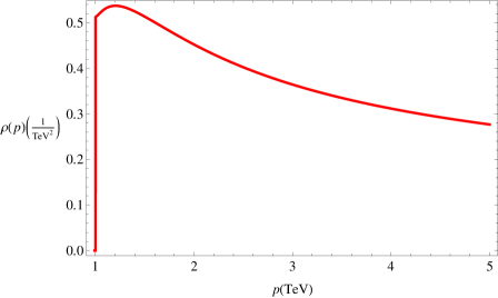
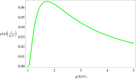
Figure 1: Continuum spectral density function with $\epsilon=10^{-19}\;\rm{GeV}^{-1}$ and $\mu=1$ TeV, as a function of momenta $p$ in TeV. In the first example (red curve) $c=-0.3$ and in the second example (green curve) $c=0.3$.

In the region $c>1/2$, for small $\epsilon$, the correlator reduces after proper rescaling to,

$$\Delta_{s}^{-1}\approx p^{2}\left(\frac{\Gamma(2c-1)}{\Gamma(2c)}+\epsilon^{2c-1}\frac{2^{-1+2c}(\mu^{2}-p^{2})^{-1/2+c}\,\Gamma(1-2c)\Gamma(c+\frac{c\mu}{\sqrt{\mu^{2}-p^{2}}})}{\Gamma(2c)\Gamma(1-c+\frac{c\mu}{\sqrt{\mu^{2}-p^{2}}})}\right)\,.$$ (34)

and in the limit $\epsilon\rightarrow 0$ we get,

$$\Delta_{s,c}\approx\frac{2c-1}{p^{2}}\,.$$ (35)

Notice that there is still a massless pole, corresponding to a free field in the CFT. On the other hand, when $c<-1/2$, after proper normalization, we find,

$$\Delta_{s} \approx -\frac{2(p^{2}-\mu(\mu+\sqrt{\mu^{2}-p^{2}}))\Gamma(-1-2c)\Gamma(1-c+\frac{c\mu}{\sqrt{\mu^{2}-p^{2}}})}{p^{2}\,\epsilon^{-1-2c}\Gamma(1-2c)\Gamma(-c+\frac{c\mu}{\sqrt{\mu^{2}-p^{2}}})}$$ (36)

$$+ \frac{2^{1-2c}(\mu^{2}-p^{2})^{1/2-c}\Gamma(2c)\Gamma(1-c+\frac{c\mu}{\sqrt{\mu^{2}-p^{2}}})}{p^{2}\Gamma(1-2c)\Gamma(c+\frac{c\mu}{\sqrt{\mu^{2}-p^{2}}})}$$

which in the limit $p^{2}\rightarrow 0$ reduces to,

$$\Delta_{s}\approx\frac{1}{\epsilon^{-1-2c}(1+2c)}+\frac{2^{1-2c}\mu^{1-2c}}{p^{2}\Gamma(1-2c)}\,.$$ (37)

Notice there is a UV sensitivity that can be cancelled by adding a proper SUSY term in the boundary action [15]. The massless pole always remains in the spectrum, even in the CFT limit $\epsilon$. Furthermore, its existence depends completely on $\mu$, since when $\mu$ vanishes the massless pole disappears from the spectrum.

4 SUSY breaking

Now we introduce SUSY breaking on the boundary by means of a scalar mass term,

$$\delta S=\frac{1}{2}\int{d^{4}x}\left(\frac{R}{z_{UV}}\right)^{3}\int{dz\left({m^{2}z_{UV}\cdot\phi^{*}\phi+h.c.}\right)}\delta(z-z_{UV})\,.$$ (38)

The mass $m$ has dimension one, since a scalar field has dimensions $d[\phi]=3/2$. This new term has the effect of modifying the boundary conditions, which now take the form,

$$F_{c}(z_{UV})=F_{c}^{0}+m^{2}z_{UV}\,\phi^{*}(z_{UV}),\qquad\psi(z_{UV})=\psi^{0},\qquad\phi_{c}(z_{UV})=\phi_{c}^{0}$$ (39)

Using Eq. (8), Eq. (19) and Eq. (38), we find that $\Sigma_{F_{c}}$ now corresponds to,

$$\Sigma_{F_{c}}(p^{2})=\left(\frac{R}{z_{UV}}\right)^{3}\frac{f_{L}}{pf_{R}-m^{2}\,z_{UV}f_{L}}\,.$$ (40)

As was done in the previous section, we study the new scalar propagator modified by SUSY breaking in the CFT limit $\epsilon\rightarrow 0$. In this case, in the region of bulk mass, $-1/2<c<1/2$, after proper normalization of the correlator, we find,

$$\Delta_{s}^{-1}(p^{2})\approx m^{2}\epsilon^{1-2c}-\frac{p^{2}}{2c-1}\epsilon^{1-2c}-\frac{2^{-1+2c}p^{2}(\mu^{2}-p^{2})^{-1/2+c}\Gamma(1-2c)\Gamma(c+\frac{c\mu}{\sqrt{\mu^{2}-p^{2}}})}{\Gamma(2c)\Gamma(1-c+\frac{c\mu}{\sqrt{\mu^{2}-p^{2}}})}$$ (41)

In the limit when $p^{2}\ll\mu^{2}$ we can easily solve for the new displaced poles. In this case, we find that the pole which was at zero momentum in the SUSY conserving action has been displaced to a non-zero value due to the SUSY breaking mass term we added to the scalar action. The new pole location is at

$$p^{2}_{pole}=\frac{2(2c-1)m^{2}(\mu\epsilon)^{1-2c}}{(-4^{c}+2^{1+2c}c)\Gamma(1-2c)}.$$ (42)

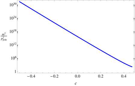
Figure 2: Plot of $m^{2}/p^{2}_{pole}$ vs $c$. Notice that as $c$ gets closer to $1/2$, for a given value of $p^{2}_{pole}$, the value of $m^{2}$ decreases.

We plot in Fig. 2 the dependence of the ratio $m^{2}/p^{2}_{pole}$ as a function of the constant bulk mass $c$. An important thing to notice is that as $c$ goes from $-1/2$ to $1/2$, for a given value of $p^{2}_{pole}$, the necessary value of $m^{2}$ decreases. This is easy to understand, since as $c$ becomes negative, the zero-mode profile,

$$f_{L,0}\propto e^{-\mu z}z^{-c},$$ (43)

is less localized near the UV brane and therefore is less affected for a given SUSY breaking mass $m$. In Fig. 3 we give a specific example of how the pole shifts for a given SUSY breaking mass; the position of the pole is given by the zero of the inverse correlator.

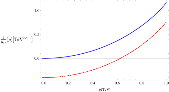
Figure 3: Inverse correlator in the case of positive $c$ with, $m=0$ GeV (blue curve, solid) and $m=4\times 10^{7}$ GeV (red curve, dashed), $\epsilon=10^{-19}\;\rm{GeV}^{-1}$, $\mu=1$ TeV and $c=0.2$. Notice how the pole has shifted from $p^{2}=0$ at $m=0$ to $p^{2}\approx 600\;\rm{GeV}^{2}$ at $m=4\times 10^{7}$ GeV.

For $c>0$, the zero mode is the only pole below the continuum. As $m$ increases, the zero-mode pole moves closer into the continuum with which it eventually merges. Thus, we see that one possibility is a superpartner which only has a continuum spectrum, i.e., unparticle behavior. This has important consequences for phenomenology which will be briefly discussed later. We can get an approximate analytical expression for the displaced zero mode poles in the vicinity of $p\approx\mu$. For that, we solve Eqs.(21-22) with the constraint of Eq.(19-20) for $p=\mu-\zeta$, with $\zeta\ll\mu$. Replacing the solutions in Eq.(40) and analyzing the result in the CFT limit, $\epsilon\rightarrow 0$, we find that the pole, in the case of $0<c<1/2$, has shifted to

$$p_{pole\approx\mu}=\frac{\mu}{2}-\frac{1}{2}\left(\frac{(1-2c)m^{2}}{\mu}-\frac{4^{c}c^{2c}\epsilon^{-1+2c}\mu^{2c}\Gamma(2-2c)}{\Gamma(1+2c)}\right),$$ (44)

so for

$$m^{2}\gtrsim\frac{\mu^{2}}{1-2c}\left[\frac{4^{c}c^{2c}\Gamma(2-2c)(\mu\epsilon)^{2c-1}}{\Gamma(1+2c)}-1\right]$$ (45)

the zero mode merges into the continuum. The value of the SUSY-breaking mass on the UV boundary where the pole just merges into the continuum as a function of $c$ is plotted in Fig. 4.

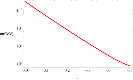
Figure 4: SUSY-breaking mass vs bulk constant mass parameter $c$, such that the zero mode pole exactly merges with the continuum. In this example, $\mu=1$ TeV and $\epsilon=10^{-19}\;\rm{GeV}^{-1}$.

The shape of the continuum spectrum is also modified in the presence of a SUSY breaking mass term. As mentioned previously, we normalized with respect to the SM fields pole residues. We plot the spectral density functions for several different SUSY-breaking masses in Fig. 5. We see that the peak shifts to larger values of momenta with increasing values of $m$, in particular after the pole merges with the continuum.

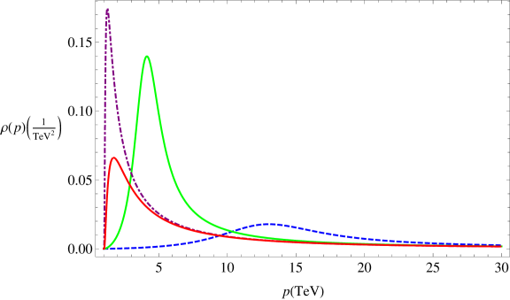
Figure 5: Spectral function for four examples of boundary UV SUSY breaking masses $m=2\times 10^{7}$ GeV (blue curve, dashed), $m=8\times 10^{6}$ GeV (green curve, solid), $m=2\times 10^{6}$ GeV (purple curve, dot-dashed) and $m=10^{5}$ GeV (red curve, dotted). The red and purple curves correspond to zero-mode poles localized at $p\approx 50$ GeV (red curve) and $p\approx 950$ GeV (purple curve), that haven’t merged with the continuum. On the other hand, the green and blue curves correspond to the cases where the pole has merged into the continuum. In the examples, $\epsilon=10^{-19}\;\rm{GeV}^{-1}$, $\mu=1$ TeV and $c=0.3$. We can see how the continuum peaks to higher momenta as the SUSY breaking mass $m$ increases, specially as the pole merges into the continuum.

For $c<0$, there are also resonant KK-like states below the continuum besides the zero mode. Looking at Eq. (41), we notice that as $m^{2}$ increases, the resonant KK-like states for $c<0$ will also move towards the continuum. However, they never disappear into the continuum as the last term in Eq. (41) can become arbitrarily large, when $c+(c\mu)/(\sqrt{\mu^{2}-p^{2}})$ gets close to a negative integer, to compensate the first term independently of how large $m$ is. It is difficult to obtain an analytical expression for the displaced poles. However we can see the effects numerically as shown in Fig. 6, where the poles are given by the positions of the zeroes in the plot.

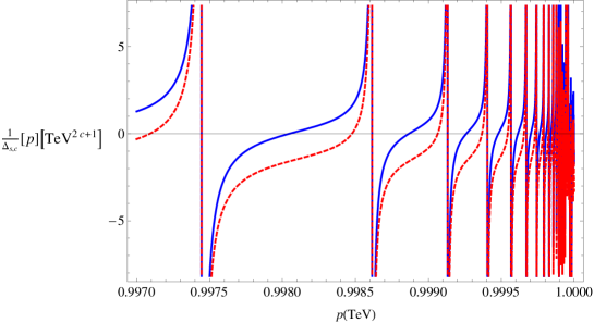
Figure 6: Inverse correlator for two examples of boundary UV SUSY breaking masses: $m=10^{13}$ GeV (blue curve) and $m=2\times 10^{14}$ GeV (red curve, dashed). In the examples, $\epsilon=10^{-19}\;\rm{GeV}^{-1}$, $\mu=1$ TeV and $c=-0.2$. We can see how the series of poles shift into the continuum with increasing values of m.

We can obtain an approximate analytical expression for the shift of the KK-like resonances below the continuum for $c<0$ in the limit that the first term in Eq.(41) dominates over the second term. In that case we expect small modifications to the SUSY spectrum and we find that the following relationship is satisfied,

$$1-c+\frac{c\mu}{\sqrt{\mu^{2}-p^{2}}}=-n+C~{},$$ (46)

where the constant $C$ is given by,

$$C=\frac{(-1)^{n+1}4^{-c}(1+n)c^{-2c}\Gamma(2c)}{(1-2c+n)\Gamma(-2c)\Gamma(2+n)^{2}(1+c+n)^{-1-2c}}\left(\frac{m^{2}}{\mu^{2}}\right)(\epsilon\mu)^{1-2c}~{}.$$ (47)

Notice that for $m^{2}\rightarrow 0$, $C$ vanishes, recovering the unperturbed solution.

Again, for completeness we analyze the case $c>1/2$. We find that the correlator, in the limit $\epsilon\rightarrow 0$ reduces to,

$$\Delta_{s}^{-1}(p^{2})\approx m^{2}-\frac{p^{2}}{2c-1}~{}.$$ (48)

where the pole has shifted as expected. For $c<-1/2$, after proper normalization, we find,

$$\Delta_{s}(p^{2}) \approx \frac{1}{(1+2c)\epsilon^{-2c-1}}+\frac{2^{1-2c}\mu^{1-2c}}{p^{2}\,c(2+4c+(-2m^{2}+(1+2c)\mu^{2})\epsilon^{2})\Gamma(-1-2c)}$$ (49)

where once again we notice how the pole has been displaced by the non-zero soft mass. In the exact CFT limit we notice a UV sensitivity as we found previously for this region of parameter space in the SUSY case.

5 Gauge fields

In this section we discuss the gauge fields. As was shown in [14], a 4D ${\mathcal{N}}=2$ vector supermultiplet can be decomposed into an ${\mathcal{N}}=1$ vector supermultiplet $V=(A_{\mu},\lambda_{1},D)$ and a chiral ${\mathcal{N}}=1$ supermultiplet $\sigma=((\Sigma+iA_{5})/\sqrt{2},\lambda_{2},F_{\sigma})$. We cannot proceed as before by introducing a bulk mass term for the gauge fields since this would break gauge invariance. Thus, we add a dilaton superfield interaction that softly breaks the conformal symmetry in the IR. This has also the consequence of providing a correct match between the 4D effective gauge coupling with the 5D gauge coupling in the limit of $z_{IR}\rightarrow+\infty$ as was shown in [12]. We therefore write the bulk action for the vector supermultiplet as [14],

$$S_{V}=$$

$$\int{d^{4}xdz\cdot\frac{R}{z}\left\{{\frac{1}{4}\int{d^{2}\theta}W_{\alpha}W^{\alpha}\Phi+h.c.+\frac{1}{2}\int{d^{4}\theta\left({\partial_{z}V-\frac{R}{z}\frac{{(\sigma+\sigma^{\dagger})}}{{\sqrt{2}}}}\right)^{2}}}\left(\Phi+\Phi^{\dagger}\right)\right\}}\,,$$

and assume that the dilaton superfield acquires a VEV in its scalar component, $\left\langle\Phi\right\rangle=e^{-2uz}/g_{5}^{2}$. In order to obtain the same expressions as those found in [22], we rescale the fields as, $A_{5}\to\frac{z}{R}A_{5}$, $\lambda_{1}\to\left({\frac{R}{z}}\right)^{3/2}\lambda_{1}$ and $\lambda_{2}\to i\left({\frac{R}{z}}\right)^{1/2}\lambda_{2}$ and get the bulk action in components. The action for the bosonic component fields $(A_{M},\Sigma,D)$ is given by,

$$S_{B} = \int{d^{5}x}\frac{R}{z}\cdot\frac{e^{-2uz}}{g_{5}^{2}}\cdot\left(-\frac{1}{{4}}F_{\mu\nu}F^{\mu\nu}-\frac{1}{{2}}\left({\partial_{z}A_{\mu}}\right)^{2}+\partial_{z}A_{\mu}\partial^{\mu}A_{5}-\frac{1}{{2}}\left({\partial_{\mu}A_{5}}\right)^{2}\right.$$ (51)

$$+ \left.\frac{1}{2}\left(\frac{R}{z}\right)^{2}\cdot\Sigma\partial_{\mu}\partial^{\mu}\Sigma-\frac{R}{z}\cdot\Sigma\partial_{z}D+\frac{1}{2}D^{2}+\bar{F}_{\sigma}F_{\sigma}\left(\frac{R}{z}\right)^{2}\right)$$

As can be seen in Eq. (51), there is a mixing term between $A_{\mu}$ and $A_{5}$. We can add a gauge fixing term to remove such mixing,

$$S_{GF}=-\int{d^{5}x\frac{R}{z}\cdot\frac{e^{-2uz}}{g_{5}^{2}}\cdot\frac{1}{2}}\left(\partial_{\mu}A^{\mu}+\frac{z}{R}\partial_{z}\left(\frac{R}{z}A_{5}\right)-2u\;A_{5}\right)^{2}$$ (52)

which corresponds to the unitary gauge in our model. Substituting $\Phi$ by its VEV in the lagrangian, we find that the longitudinal components of the excited gauge bosons states $A_{\mu}$ are related to the scalar field $A_{5}$ in the following way:

$$p^{\mu}A_{\mu}(p,z)+\left(\partial_{z}-\frac{1}{z}-2u\right)A_{5}(p,z)=0.$$ (53)

The auxiliary fields $F_{\sigma}$ and $D$ can be integrated out using their equations of motion,

$$F_{\sigma}=0,\qquad\qquad D=-\frac{R}{z}\left(\partial_{z}-\frac{2}{z}-2u\right)\Sigma\,.$$ (54)

We would like to concentrate on the gaugino sector and study the effects of SUSY breaking on the spectrum. For that purpose, we calculate the gaugino bulk action,

$$S_{F} = \int{d^{5}x}\left({\frac{R}{z}}\right)^{4}\cdot\frac{e^{-2uz}}{g_{5}^{2}}\cdot\left[-i\lambda_{1}\sigma^{\mu}\partial_{\mu}\bar{\lambda}_{1}-i\lambda_{2}\sigma^{\mu}\partial_{\mu}\bar{\lambda}_{2}+\frac{1}{2}\lambda_{2}\overleftrightarrow{\partial_{z}}\lambda_{1}\right.$$ (55)

$$- \left.\frac{1}{2}\bar{\lambda}_{1}\overleftrightarrow{\partial_{z}}\bar{\lambda}_{2}+\frac{1}{z}\left(\frac{1}{2}+uz\right)\lambda_{1}\lambda_{2}+\frac{1}{z}\left(\frac{1}{2}+uz\right)\bar{\lambda}_{1}\bar{\lambda}_{2}\right].$$

As can be seen in Eq. (55), the dilaton field modifies the gaugino mass term, introducing a $z$-dependent bulk mass which leads to a mass gap in the continuum, as we found for the matter fields. As a matter of fact, this action is exactly analogous to the fermion matter field action in the case $c=1/2$.

By analogy with the matter fields, we can construct in a simple manner the solutions to the 5D profiles after rescaling all component fields by a factor $e^{uz}$,

$$\lambda_{1}(p,z) = \chi_{\rm{4}}(p)e^{uz}\left(\frac{z}{z_{UV}}\right)^{2}h_{L},\quad A_{\mu}(p,z)=A_{\mu 4}(p)e^{uz}\left(\frac{z}{z_{UV}}\right)^{1/2}h_{L},$$ (56)

$$\lambda_{2}(p,z) = \psi_{\rm{4}}(p)e^{uz}\left(\frac{z}{z_{UV}}\right)^{2}h_{R},\quad\Sigma=\phi_{4}(p)e^{uz}\left(\frac{z}{z_{UV}}\right)^{3/2}h_{R}\,,$$ (57)

where $h_{L,R}$ represents $f_{L,R}$ evaluated at $c=1/2$. In the following, we assume that $\sigma(z_{UV})=0$. In this case the vector superfield acts as the source of a vector superfield CFT operator with canonical dimensions [15].

We study how SUSY breaking affects the super-vector CFT operator using the holographic language. For this purpose, we add a Majorana mass term for the $\lambda_{1}$ gauginos on the UV brane,

$$\delta S=\int{d^{4}x}\left(\frac{R}{z_{UV}}\right)^{4}\int dz(mz_{UV}\lambda_{1}\lambda_{1}+h.c.)\delta(z-z_{UV}).$$ (58)

In analogy with the matter field case, we can calculate the kinetic term for the $\lambda_{2}$ gauginos, which are related to the correlator of the fermionic CFT operator $\Delta_{f}=-\Sigma_{\lambda_{2}}$, as:

$$\Sigma_{\lambda_{2}}(p^{2})=\left(\frac{R}{z_{UV}}\right)^{4}\frac{h_{L}}{h_{R}-mz_{UV}h_{L}}\frac{p_{\mu}\sigma^{\mu}}{p}.$$ (59)

In the conformal limit $\epsilon\rightarrow 0$, the correlator takes the form,

$$\Delta_{f}\approx-\frac{1}{\gamma\,p^{2}+p^{2}\ln[2\sqrt{u^{2}-p^{2}}\,\epsilon]-\sqrt{p^{2}}\,m}\,\,p_{\mu}\sigma^{\mu}\,,$$ (60)

where the pole, in the case $p\ll\mu$, is localized at,

$$p^{2}_{pole}=\frac{m^{2}}{\left(\gamma+\ln[2\,u\,\epsilon]\right)^{2}}.$$ (61)

In the case $m^{2}=0$ the pole is localized at zero momenta as expected. The continuum spectra starts at momenta $p>u$. As an example, for $u=1$ TeV, $\epsilon=10^{-19}$ $\rm{GeV}^{-1}$ and $m=40$ TeV, the pole merges with the continuum.

6 Phenomenology and Conclusions

In this paper we discussed a novel possibility for supersymmetric extensions of the Standard Model, where there are continuum excitations of the SM fields and their superpartners arising from conformal dynamics. Using the AdS/CFT correspondence we can explicitly construct the models and explore the properties of the continuum states. In the supersymmetric limit, the SM particles and their superpartners are zero modes in the 5D theory, and there is a continuum excitation for each of them starting at some mass gap due to conformal breaking in the infrared. After SUSY breaking, the zero-mode superpartners acquire SUSY-breaking masses and are lifted from the massless spectrum. For large enough SUSY breaking, the superpartner may merge into the continuum and there is no longer a well-defined superpartner state of a definite mass. In the simple setup considered in this paper where SUSY breaking is localized on UV brane, the mass gap for the continuum governed by the infrared conformal breaking does not change due to locality in the extra dimension, but the shape of the spectral density is modified by SUSY breaking. One can imagine that in a more general setup, the continuum excitations of the SM particles and their superpartners will have different mass gaps.

As we have seen in the discussions of the previous sections, the properties of superpartners can be quite different in this type of model, depending on the parameters. The superpartner of a SM particle could be either a discrete mode below a continuum, the first of a series of discrete modes, or just a continuum. The last case will of course be the most challenging to uncover experimentally. At the LHC we would expect that most of the time the superpartner is produced near the bottom of the continuum due to the fall off in parton distribution functions. It will be difficult to construct any peak or edge since there is an additional smearing of the mass by the continuous spectrum itself. If the superpartner is produced well above the threshold, then there is also the possibility of extended decay chains. This arises when the superpartner decays to another state, if the new state is above the original threshold, then it can decay back to the original superpartner, just at a lower point in the continuum spectrum. These events are expected to have large multiplicities and more spherical shapes, as a reflection of the underlying conformal theory [23]. The collider phenomenology of such models is currently under investigation. Serious work will need to be done to extend current LHC analysis to cover this type of new physics.

Appendix: Wavefunctions

We now obtain the spectrum by solving for the wavefunctions of the modes. As mentioned before in the text, the general solution to the EOM is a linear combination of Whittaker functions of the first and second order. Now if we consider a left-handed zero mode which therefore has a Neumann (even) boundary condition at the UV brane, the accompanying right-handed solution has a Dirichlet (odd) boundary condition at the same brane. Furthermore, for momenta smaller than the mass gap, the wavefunction is normalizable in the sense that it is squared integrable when the IR branes is taken to infinity. Thus we have,

$$f_{R}(p,\epsilon)=0,\quad\quad\int^{\infty}_{\epsilon}\left(\frac{R}{z}\right)^{\beta}|\left(\frac{z}{\epsilon}\right)^{\alpha}f_{R}(p,z)|^{2}\frac{1}{\epsilon}\;dz=1\,,$$ (62)

where for fermions $\beta=4$ and $\alpha=2$, and for scalars $\beta=3$ and $\alpha=3/2$. These two conditions completely fix the solution to the EOM and the spectrum for momenta smaller than the mass gap.

There are two independent solutions to the second order equations of motion, $M(\kappa,m,\zeta)$ and $M(\kappa,-m,\zeta)$. These two solutions tend to diverge as $z\rightarrow+\infty$. However one can construct a linear combination of them which is exponentially decaying as $z\rightarrow+\infty$. This linear combination turns out to be the Whittaker function of the second kind, $W(\kappa,m,\zeta)$, defined through Eq. (18). The condition of normalizability forces us to drop the divergent component $M(\kappa,m,\zeta)$ in Eq. (15) and only keep $W(\kappa,m,\zeta)$.

Let us analyze how the expected massless pole arises by inspecting Eq. (15) in the limit $p\rightarrow 0$. From the solution to Eq. (19), which is always normalizable for $\mu>0$, independent of the value of $c$, we expect to always find a solution to Eq. (62) for vanishing momentum, $p$, and positive $\mu$. This in fact, turns out to be always the case since the pre-factor $p/(\mu+\sqrt{\mu^{2}-p^{2}})$ in the second term of Eq. (15) vanishes at $p=0$ and furthermore for non-vanishing $\epsilon$, $W(-c,-1/2+c,2|\mu|\epsilon)$ is regular and non-zero for any value of $c$. This important pre-factor arises when relating the normalizable solutions (for $p^{2}<\mu^{2}$) to Eqs.(21–22) by Eqs.(19–20). Thus, we see that the appearance of a massless mode, independent of the value of $c$, is very different from the previously gapless ($\mu=0$) cases analyzed in the literature [15, 16] where massless modes arise only for certain values of $c$. We thus expect that the corresponding CFT operator will always have a massless chiral mode for non-zero $\mu$. Since Eqs.(19–20) are symmetric under the exchange $m(z)\rightarrow-m(z)$ and $f_{R}\rightarrow-f_{L}$ we see that flipping the sign of $\mu$ simply flips the handedness of the zero-mode.

Now, let us concentrate for a moment on non-vanishing momenta and demand that we satisfy the UV boundary condition, $f_{R}(p,\epsilon)=0$. From the last discussion we realize we need to demand,

$$W(-\frac{c\mu}{\sqrt{\mu^{2}-p^{2}}},1/2-c,2\sqrt{\mu^{2}-p^{2}}\epsilon)=0\,.$$ (63)

To analyze this last expression, let us expand for small $\zeta$ Eq. (18) using Eq. (17), $M(\kappa,m,\zeta)\approx\zeta^{1/2+m}$,

$$W(\kappa,m,\zeta)\approx\frac{\Gamma(-2m)}{\Gamma(1/2-m-\kappa)}\zeta^{1/2+m}+\frac{\Gamma(2m)}{\Gamma(1/2+m-\kappa)}\zeta^{1/2-m}.$$ (64)

In our case, $m=1/2-c$, $\kappa=-c\mu/\sqrt{\mu^{2}-p^{2}}$ and $\zeta=2\sqrt{\mu^{2}-p^{2}}z$. The two terms then can compensate each other and we find that the following relation is satisfied,

$$\frac{{\Gamma(-1+2c)}}{{\Gamma(c+\frac{{c\mu}}{{\sqrt{\mu^{2}-p^{2}}}})}}2^{1-2c}\left(\sqrt{\mu^{2}-p^{2}}\epsilon\right)^{1-2c}+\frac{{\Gamma(1-2c)}}{{\Gamma(1-c+\frac{{c\mu}}{{\sqrt{\mu^{2}-p^{2}}}})}}=0.$$ (65)

We are interested in range $-1/2<c<1/2$, so we see that the first term in Eq. (65) vanishes as $\epsilon\rightarrow 0$. Thus, in order to satisfy the UV boundary condition, we have,

$$1-c+\frac{c\mu}{\sqrt{\mu^{2}-p^{2}}}=-n+\delta\;,n\in\mathbb{Z}_{0}^{+}\,,$$ (66)

which can only be satisfied for $c<0$. We can approximately solve for $\delta$, as the solution of,

$$\frac{{\Gamma(-1+2c)}}{{\Gamma(-1+2c-n)}}2^{1-c}\left({\frac{{c\mu}}{{-1+c-n}}z_{UV}}\right)^{1-c}+\frac{{\Gamma(1-2c)}}{{\Gamma(-n+\delta)}}2^{c}\left({\frac{{c\mu}}{{-1+c-n}}z_{UV}}\right)^{c}=0$$ (67)

and find that,

$$\delta\approx(\epsilon\mu)^{1-2c}\frac{(-1)^{n}(2c/(c-n-1))^{1-2c}\Gamma(-1+2c)}{\Gamma(1-2c)\Gamma(-1+2c-n)\Gamma(1+n)},$$ (68)

which is tiny in the limit $\epsilon\rightarrow 0$. As an example, in the case of $c=-0.2$, $\mu=200$ GeV, $\epsilon=10^{-19}\;\rm{GeV}^{-1}$ and $n=1$, we find $\delta\approx 10^{-24}$, so we can safely neglect this correction.

Neglecting $\delta$, we re-write Eq. (66) as

$$\sqrt{\mu^{2}-p^{2}}=\frac{c\,\mu}{c-1-n}.$$ (69)

So we require that $\mu>0$ for this expression to be positive (with $-1/2<~{}c~{}<0$). Solving for $p^{2}$ we obtain,

$$p^{2}=\left[1-\frac{c^{2}}{\left(1-c+n\right)^{2}}\right]\mu^{2}.$$ (70)

Analyzing this solution, we find that most resonances are localized near $p\sim\mu$ where they accumulate. We can see this by taking the limit $n\rightarrow+\infty$ in Eq. (70) and find that $p^{2}\rightarrow\mu^{2}$.

References

- [1] H. Georgi, hep-ph/0703260; hep-ph/0704.2457; H. Georgi and Y. Kats, arXiv:0904.1962 [hep-ph].
- [2] M. J. Strassler and K. M. Zurek, Phys. Lett. B 651 (2007) 374 arXiv:hep-ph/0604261.
- [3] J. Kang and M. A. Luty, arXiv:0805.4642 [hep-ph]; H. Cai, H. C. Cheng and J. Terning, JHEP 0905, 045 (2009) arXiv:0812.0843 [hep-ph].
- [4] P. J. Fox, A. Rajaraman and Y. Shirman, hep-ph/0705.3092.
- [5] G. Cacciapaglia, G. Marandella and J. Terning, arXiv:0708.0005 [hep-ph].
- [6] D. Stancato and J. Terning, arXiv:0807.3961 [hep-ph]; se also J. R. Espinosa and J. F. Gunion, Phys. Rev. Lett. 82 (1999) 1084 hep-ph/9807275; J. J. van der Bij and S. Dilcher, Phys. Lett. B 655 (2007) 183 hep-ph/0707.1817; A. Delgado, J. R. Espinosa and M. Quiros, JHEP 0710 (2007) 094 hep-ph/0707.4309; A. Delgado, J. R. Espinosa, J. M. No and M. Quiros, JHEP 0804 (2008) 028 hep-ph/0802.2680; A. Delgado, J. R. Espinosa, J. M. No and M. Quiros, hep-ph/0804.4574.
- [7] A. Falkowski and M. Perez-Victoria, arXiv:0810.4940 [hep-ph]; arXiv:0901.3777 [hep-ph].
- [8] K. Cheung, W. Y. Keung and T. C. Yuan, Phys. Rev. Lett. 99 (2007) 051803 arXiv:0704.2588 [hep-ph]. T. G. Rizzo, JHEP 0710 (2007) 044 arXiv:0706.3025 [hep-ph].
- [9] J. M. Maldacena, Adv. Theor. Math. Phys. 2, 231 (1998) [Int. J. Theor. Phys. 38, 1113 (1999)] arXiv:hep-th/9711200.
- [10] J. Scherk and J. H. Schwarz, Phys. Lett. B 82 (1979) 60.
- [11] L. Randall and R. Sundrum, Phys. Rev. Lett. 83, 4690 (1999) arXiv:hep-th/9906064.
- [12] G. Cacciapaglia, G. Marandella and J. Terning, JHEP 0902 (2009) 049, arXiv:0804.0424 [hep-ph].
- [13] A. Friedland, M. Giannotti and M. Graesser, Phys. Lett. B 678, 149 (2009) arXiv:0902.3676 [hep-th]; arXiv:0905.2607 [hep-th].
- [14] D. Marti and A. Pomarol, Phys. Rev. D 64, 105025 (2001) hep-th/0106256.
- [15] G. Cacciapaglia, G. Marandella and J. Terning, JHEP 0906 (2009) 027, arXiv:0802.2946 [hep-th].
- [16] R. Contino and A. Pomarol, JHEP 0411, 058 (2004) arXiv:hep-th/0406257.
- [17] G. Mack, Comm. Math. Phys. 55 (1977) 1; for reviews see S. Minwalla, Adv. Theor. Math. Phys. 2 (1998) 781, hep-th/9712074; J. Terning, “Modern supersymmetry: Dynamics and duality,” Oxford, UK: Clarendon (2006) p 128.
- [18] J. Bagger and A. Galperin, Phys. Lett. B 336, 25 (1994) arXiv:hep-th/9406217; Phys. Rev. D 55, 1091 (1997) arXiv:hep-th/9608177; Phys. Lett. B 412, 296 (1997) arXiv:hep-th/9707061.
- [19] P. Breitenlohner and D. Z. Freedman, “Positive Energy in Anti-de Sitter Backgrounds and Gauged Extended Supergravity,” Phys. Lett. B 115 (1982) 197; “Stability in Gauged Extended Supergravity,” Ann. Phys. 144 (1982) 249.
- [20] A. Falkowski, talk given at UC Davis, Jan. 26, 2008.
- [21] S. B. Giddings, E. Katz and L. Randall, JHEP 0003, 023 (2000) arXiv:hep-th/0002091.
- [22] T. Gherghetta and A. Pomarol, Nucl. Phys. B 586, 141 (2000) hep-ph/0003129.
- [23] M. J. Strassler, arXiv:0801.0629 [hep-ph]; J. Polchinski and M. J. Strassler, JHEP 0305, 012 (2003) arXiv:hep-th/0209211; D. M. Hofman and J. Maldacena, JHEP 0805, 012 (2008) arXiv:0803.1467 [hep-th]; Y. Hatta, E. Iancu and A. H. Mueller, JHEP 0805, 037 (2008) arXiv:0803.2481 [hep-th]; C. Csaki, M. Reece and J. Terning, JHEP 0905 (2009) 067 arXiv:0811.3001 [hep-ph].