5D gravitational waves from complexified black rings

Abstract

In this paper we construct and briefly study the 5D time-dependent solutions of general relativity obtained via double analytic continuation of the black hole (Myers-Perry) and of the black ring solutions with a double (Pomeransky-Senkov) and a single rotation (Emparan-Reall). The new solutions take the form of a generalized Einstein-Rosen cosmology representing gravitational waves propagating in a closed universe. In this context the rotation parameters of the rings can be interpreted as the extra wave polarizations, while it is interesting to state that the waves obtained from Myers-Perry Black holes exhibit an extra boost-rotational symmetry in higher dimensions which signals their better behavior at null infinity. The analogue to the C-energy is analyzed.

I Introduction

The formulation of string theory in time-dependent backgrounds presents a particularly challenging problem, although progress can be achieved by considering some simple time-dependent solutions. As a step in this direction, a class of time-dependent backgrounds has been investigated recently Aharoni ; those spacetimes were obtained from a double analytic continuation of asymptotically flat black holes, and describe the Lorentzian evolution of a bubble. The technique of double analytic continuation was originally developed to study the stability of the Kaluza -Klein vacuum Witten , see also Dowker . This technique has also been used in the formulation of a positive energy theorem for anti-de Sitter space Horowitz , and discussed within the context of brane world scenarios Ida , and M-theory Costa-Fabi . Similar techniques were also used in Piran , to obtain cylindrical gravitational waves with variable polarization by starting with Kerr solution describing a rotating black hole.

The phenomena involving gravitational waves are under intense investigation, in preparation for the upcoming expected observational data provided by the gravitational wave detectors. Hystorically, the most often theoretically studied spacetime interpreted as containing propagating gravitational radiation is that of the Einstein-Rosen metric Carmeli .

In this paper we are interested in studying a class of solutions obtained by a double analytic continuation of the known 5-D black ring spacetimes. Here, black ring solutions are carried, by a Wick rotation, to generalized Einstein-Rosen spacetimes. The obtained in such a way solutions can be interpreted as cylindrical gravitational waves in 5 dimensions, as well as inhomogeneous 5-D universes. These may also serve as interaction regions of plane five dimensional gravitational waves which collide and focus on either a strong curvature singularity or a Cauchy horizon. The colliding wave re-interpretations are possible similarly to the standard 4-dimensional case due to the solitonic structure of the original solutions in the sense that the solitonic terms would provide the possibility of the continuation of the solutions into the plane wave regions FeinIb . While the practical interest of the solutions in rather remote, they may serve as time-dependent backgrounds for superstring propagation, as well as can be easily connected to the so-called Pre-Big-Bang scenario solutions by dressing them with a massless dilaton field. They may also serve as test beds for numerical relativity.

A different issue we address is that of the so called C-energy in radiative spacetimes; this quantity, in certain sense, measures the amount of gravitational energy carried by the waves towards infinity.

To transform the black ring solutions to the Einstein-Rosen form, we introduce the technique of the double analytic continuation for metrics involving polynomials of third and fourth degree as denominators; in the process, elliptic integrals and Jacobi functions come up.

In the following section II the double analytic continuation for the Myers-Perry black hole solution is considered and in Sec. III the solution of black ring with a double rotation is continued analytically, obtaining an extra polarization for the gravitational waves. The subsequent section IV deals with the special case for which one of the rotation parameters is switched off and the analogue of the Emparan-Reall ring is obtained. For all the cases we calculate the analogue to C-energy and present plots for the energy density and energy flux. Finally, some conclusions are drawn in the last section.

II Gravitational waves from Myers-Perry black hole

In this section, as a first step, the Myers-Perry 5D black hole solution Myers is transformed via a Wick rotation into a hypercylindrical time-dependent spacetime.

We shall start with the Myers-Perry solution with one angular momentum, in the coordinates $(\rho,\theta,t,\phi,\psi)$

$$ds^{2}=-dt^{2}+\frac{\rho_{0}^{2}}{\Sigma}(dt-a\sin^{2}{\theta}d\phi)^{2}+(\rho^{2}+a^{2})\sin^{2}{\theta}d\phi^{2}+\rho^{2}\cos^{2}{\theta}d\psi^{2}+\frac{\Sigma}{\Delta}d\rho^{2}+\Sigma d\theta^{2},$$ (1)

where $\Delta=\rho^{2}-\rho_{0}^{2}+a^{2}$ and $\Sigma=\rho^{2}+a^{2}\cos^{2}{\theta}$.

With $\rho={\tilde{R}}+\frac{\rho_{0}^{2}-a^{2}}{{4\tilde{R}}}$, we transform the sector

$\Sigma\left(\frac{d\rho^{2}}{\Delta}+d\theta^{2}\right)\mapsto\frac{\Sigma}{{\tilde{R}}^{2}}\left(d{\tilde{R}}^{2}+{\tilde{R}}^{2}d\theta^{2}\right)$

Followed by the transformations

$r={\tilde{R}}\sin{\theta},\quad z={\tilde{R}}\cos{\theta},\quad{\tilde{R}}^{2}=r^{2}+z^{2}$

the $({\tilde{R}},\theta)$ sector is transformed into

$\frac{\Sigma}{{\tilde{R}}^{2}}\left(d{\tilde{R}}^{2}+{\tilde{R}}^{2}d\theta^{2}\right)\mapsto\frac{\Sigma}{{\tilde{R}}^{2}}(dr^{2}+dz^{2}).$

Applying now the Wick rotation $t\rightarrow iz$ and $z\rightarrow it$, along with $a\mapsto ia$, the metric (1) becomes a time-dependent solution to the vacuum Einstein equations

$$dS^{2} = \frac{\Sigma}{\tilde{R}^{2}}(dr^{2}-dt^{2})+dz^{2}-\frac{\rho_{0}^{2}}{\Sigma}\left({dz-\frac{ar^{2}}{\tilde{R}^{2}}d\phi}\right)^{2}+(\rho^{2}-a^{2})\frac{r^{2}}{\tilde{R}^{2}}d\phi^{2}-\frac{\rho^{2}t^{2}}{\tilde{R}^{2}}d\psi^{2}$$ (2)

$$= \frac{\Sigma}{(r^{2}-t^{2})}(dr^{2}-dt^{2})+\gamma_{ab}dx^{a}dx^{b},$$

where $\Sigma=\rho^{2}+\frac{a^{2}t^{2}}{{\tilde{R}}^{2}}$, $\rho={\tilde{R}}+\frac{\mu^{2}}{{4\tilde{R}}}$, ${\tilde{R}}=\sqrt{r^{2}-t^{2}}$ and $\mu^{2}=\rho_{0}^{2}+a^{2}$. Notice that $\psi$ now became a timelike coordinate that can be made spacelike with $\psi\to i\psi$. The line element (2) is of the form of a 5D generalized Einstein-Rosen metric,

$$ds^{2}=e^{f}(d\rho^{2}-dt^{2})+\gamma_{ab}dx^{a}dx^{b},$$ (3)

where $x^{a}$ denote the Killing coordinates, $z,\phi,\psi$.

On the other hand, from harmark we know that

det$\gamma_{ab}=-\frac{\rho^{2}}{4}\Delta\sin^{2}{2\theta}=-\rho^{2}\Delta\sin^{2}{\theta}\cos^{2}{\theta}$, which after the transformations becomes

$${\rm det}\gamma_{ab}=\left(1-\frac{\mu^{4}}{16{\tilde{R}}^{4}}\right)^{2}r^{2}t^{2}.$$ (4)

Being

$$G=\sqrt{{\rm det}\gamma_{ab}}=\left(1-\frac{\mu^{4}}{16{\tilde{R}}^{4}}\right)rt,$$ (5)

and the norm of the gradient of the transitivity surface amounts to

$$G_{\mu}G^{\mu}=\frac{r^{2}-t^{2}}{\Sigma}(G_{,r}^{2}-G_{,t}^{2})=\frac{1}{\Sigma}\left[-(t^{2}-r^{2})^{2}-\frac{\mu^{8}-16^{2}\mu^{4}r^{2}t^{2}}{16^{2}(r^{2}-t^{2})^{2}}+\frac{\mu^{4}}{8}\right],$$ (6)

At this point it is convenient to perform yet another transformation to null coordinates $(u,v)$ given by $u=r-t,v=r+t$, that puts the line element Eq. (2)) into:

$$ds^{2}=\frac{\Sigma}{uv}dudv+dz^{2}-\frac{\rho_{0}^{2}}{\Sigma}\left(dz+a\frac{(v+u)^{2}}{4uv}d\phi\right)^{2}+(\rho^{2}-a^{2})\frac{(v+u)^{2}}{4uv}d\phi^{2}-\rho^{2}\frac{(v-u)^{2}}{4uv}d\psi^{2},$$ (7)

where

$$\rho^{2}=uv+\frac{\mu^{2}}{2}+\frac{\mu^{4}}{16uv},\quad\Sigma=\left(\sqrt{uv}+\frac{\mu^{2}}{4\sqrt{uv}}\right)^{2}+\frac{a^{2}(v-u)^{2}}{4uv}.$$ (8)

Then in $(u,v)$-coordinates the norm $G_{\mu}G^{\mu}$ takes the form

$$G_{\mu}G^{\mu}=\frac{2uv}{\Sigma}G_{,u}G_{,v}=-\frac{1}{\Sigma}\frac{(\mu^{4}-16u^{4})(\mu^{4}-16v^{4})}{2(16)^{2}u^{2}v^{2}}.$$ (9)

From the previous expression we see that the spacetime is clearly separated into four regions (see Fig. 1) where different interpretations apply.

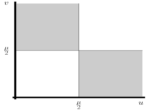
Figure 1: The shaded regions correspond to the cylindrically symmetric spacetimes, where $G^{\mu}G_{\mu}>0$. The regions are separated by the lines $u=\mu/2$ and $v=\mu/2$ where $G^{\mu}G_{\mu}=0$. In the white regions $G^{\mu}G_{\mu}<0$

Since $\Sigma>0$, the sign of $G_{\mu}G^{\mu}$ depends on the ratios of $u/\mu$ and $v/\mu$. These regions are separated by $u=\mu/2$ and $v=\mu/2$: For $u=\frac{\mu}{2}$ or $v=\frac{\mu}{2}$, $G_{\mu}G^{\mu}=0$ and it separates the regions where ($u>\frac{\mu}{2}$ and $v>\frac{\mu}{2}$) or ($u<\frac{\mu}{2}$ and $v<\frac{\mu}{2}$) where $G_{\mu}G^{\mu}<0$ and can be interpreted as gravitational waves propagating in a cosmological background; while if ($u>\frac{\mu}{2}$ and $v<\frac{\mu}{2}$) or ($u>\frac{\mu}{2}$ and $v<\frac{\mu}{2}$), $G_{\mu}G^{\mu}>0$ that corresponds to cylindrical waves.

The previous statement can be posed in terms of trapped surfaces. Considering fixed coordinates $x^{a}=\{u,v\}$, the invariant $\kappa$, Seno , is given by

$$\kappa_{u,v}=\frac{2u^{2}v^{2}}{(u^{2}-v^{2})^{2}}\frac{(\mu^{4}-16u^{4})(\mu^{4}-16v^{4})}{\Sigma(\mu^{4}-16u^{2}v^{2})^{2}}$$ (10)

We notice that the Killing orbits vanish at $u=v$ as well as at $u=-v$ corresponding to $t=0$ and $r=0$, therefore this spacetime has a singularity at $t=0$ as well as cylindrical axes at $r=0$. However, the singularity at $t=0$ is of a Taub-NUT type, rather than a strong curvature singularity, and the spacetime may be extended across the hypersurface $t=0$ as in Taub-NUT, but the extension is not unique Misner . Moreover, whenever $\kappa$ is everywhere negative (no zeroes), the spacetime (7) does not possess neither marginally (no horizons), nor trapped surfaces, therefore the solution (7) can be interpreted as cylindrical gravitational waves in those regions. On the other hand, in the regions where $G_{\mu}G^{\mu}<0$ and $\kappa>0$ trapped surfaces do exist with the possibility that null congruences converge to a singularity. Both regions are separated by the surfaces where $u=\mu/2$ or $v=\mu/2$ .

In the 4D section of the regions where $G_{\mu}G^{\mu}>0$, therefore, we have a cylindrically symmetric spacetime and the expression for the energy derived by Brown-York Goncalves should make sense. One would also expect the existence of a conical deficit along the angular coordinate. Being the $E$-energy for the spacetime (7)

$$4E=1-e^{-f/2}=1-\sqrt{\frac{uv}{\Sigma}},$$ (11)

At infinity $\Sigma\to\infty$, then as $v\to\infty$ (or $u\to\infty$), the energy tends to a constant, $E(\infty)=1/4$. Accordingly, at infinity the energy flux and density, $E_{,t}$ and $E_{,r}$, tend to zero.

Moreover, in the limit that $\mu\to 0$ ( $a\to 0$ and $\rho_{0}\to 0$) the whole spacetime contains cylindrical gravitational waves, and looks like

$$ds^{2} = dudv+dz^{2}-\frac{(v-u)^{2}}{4}d\psi^{2}+\frac{(v+u)^{2}}{4}d\phi^{2}$$ (12)

$$= dr^{2}-dt^{2}+dz^{2}+t^{2}d\psi^{2}+r^{2}d\phi^{2},$$

Here we have complexified the $\psi$ coordinate to have a standard signature. In fact, because of the above flat Kasner form of the 5-D metric, what one obtains here is the first example of the so-called boost-symmetric spacetime in higher dimensions Bicak , see also Gowdy2 , and may represent radiation generated by accelerated sources in extra dimensions. It is interesting that if one generates cylindrical waves in a similar manner from a four dimensional black hole, no boost-symmetry is apparently present, it appears in the 5th-dimension due to the coupling of the radiation to the extra compact dimension-the term $t^{2}d\psi^{2}$ in the line element in this limit.

III The double rotating black ring analytic continuation

The starting point now is the black ring solution with two angular momenta derived by Pomeransky and Senkov (PS) pomeransky . In coordinates $(x,y,t,\phi,\psi)$ it is written as,

$$ds^{2} = \frac{H(y,x)}{H(x,y)}(dt+\Omega)^{2}+\frac{F(x,y)}{H(y,x)}d\phi^{2}+2\frac{J(x,y)}{H(y,x)}d\phi d\psi$$ (13)

$$-\frac{F(y,x)}{H(y,x)}d\psi^{2}-\frac{2K^{2}H(x,y)}{(x-y)^{2}(1-\nu)^{2}}\left(\frac{dx^{2}}{G(x)}-\frac{dy^{2}}{G(y)}\right).$$

The solution represents the general 5D black ring solution with two independent angular momenta (see analysis of PS solution in Elvang ). It depends on two coordinates: $-1\leq x\leq 1$ and $-\infty<y<-1$. The ranges of $t,\phi,\psi$ are: $-\infty<t<\infty$, $0<\phi,\psi<2\pi$; the one-form $\Omega$ is given by

$$\Omega = -\frac{2K\lambda\sqrt{(1+\nu)^{2}-\lambda^{2}}}{H(y,x)}\{(1-x^{2})y\sqrt{\nu}d\psi+$$ (14)

$$\frac{(1+y)}{(1-\lambda+\nu)}[1+\lambda-\nu+x^{2}y\nu(1-\lambda-\nu)+2\nu x(1-y)]d\phi\}$$

$$= \Omega_{1}d\psi+\Omega_{2}d\phi.$$

The functions $G,H,J,F$ are defined as:

$$G(x) = (1-x^{2})(1+\lambda x+\nu x^{2}),$$

$$H(x,y) = 1+\lambda^{2}-\nu^{2}+2\lambda\nu(1-x^{2})y+2x\lambda(1-y^{2}\nu^{2})+x^{2}y^{2}\nu(1-\lambda^{2}-\nu^{2}),$$

$$J(x,y) = \frac{2K^{2}(1-x^{2})(1-y^{2})\lambda\sqrt{\nu}}{(x-y)(1-\nu)^{2}}[1+\lambda^{2}-\nu^{2}+2\lambda\nu(x+y)-xy\nu(1-\lambda^{2}-\nu^{2})],$$

$$F(x,y) = \frac{2K^{2}}{(x-y)^{2}(1-\nu)^{2}}\{G(x)(1-y^{2})[((1-\nu)^{2}-\lambda^{2})(1+\nu)+y\lambda(1-\lambda^{2}+2\nu-3\nu^{2})]$$ (15)

$$+G(y)[2\lambda^{2}+x\lambda((1-\nu)^{2}+\lambda^{2})+x^{2}((1-\nu)^{2}-\lambda^{2})(1+\nu)$$

$$+x^{3}\lambda(1-\lambda^{2}-3\nu^{2}+2\nu^{3})-x^{4}(1-\nu)\nu(-1+\lambda^{2}+\nu^{2})]\},$$

For a regular black ring, parameters $\lambda$ and $\nu$ must satisfy the ranges $0\leq\nu<1$ and $2\sqrt{\nu}\leq\lambda<(1+\nu)$, in order to guarantee the existence of horizons, reality of the metric and positivity of the black ring mass (see Fig. 2). The Emparan-Reall rotating black ring emparan is recovered when $\nu=0$. The interpretation of the solution as a regular black ring is valid in the ranges where both, $G(x)>0$ ($-1\leq x\leq 1$) and $-G(y)>0$. The latter corresponds to two intervals: $-\infty<y<y_{4}$ and $y_{3}<y<-1$, where $y_{3}$ and $y_{4}$ are the two roots of $1+\lambda y+\nu y^{2}=0$.

Figure 2: Ranges for the parameters $\nu$ and $\lambda$ in the Pomeranski-Senkov solution, $0\leq\nu<1$ and $2\sqrt{\nu}\leq\lambda<(1+\nu)$, the shaded region represents the $\lambda$ allowed values for a given $\nu$.

To explore the time-dependent analogue of the metric (13), we transform it into a 5D generalized Einstein-Rosen (ER) form,

$$ds^{2}=e^{f}(dR^{2}-dT^{2})+\gamma_{ab}dx^{a}dx^{b},$$ (16)

where $\gamma_{ab}$ and $f$ are functions of $(R,T)$, and $x^{a}=z,\phi,\psi$ are Killing directions. The local behaviour of the solution is defined by the gradient of the element of the transitivity surface, $G_{\mu}=\partial_{\mu}({\rm det}\gamma_{ab})^{1/2}$ which can be spacelike, timelike or null. $G_{\mu}G^{\mu}$ is associated to the expansion scalar and defines the trapped 3-surfaces for fixed $(R,T)$. In case $G_{\mu}G^{\mu}>0$, the solution can be interpreted as cylindrical gravitational waves; when $G_{\mu}G^{\mu}$ varies from point to point then (16) represents gravitational waves propagating along the $R$-direction in an expanding universe.

In order to obtain the generalized ER form let us focus on the longitudinal sector to transform it as follows,

$$\left(\frac{dx^{2}}{G(x)}+\frac{dy^{2}}{[-G(y)]}\right)\mapsto(dR^{2}+d\xi^{2}).$$ (17)

The next step would be to perform the complex trick: $\xi\mapsto iT$ (this changes the sign of $d\xi^{2}$) together with $t\mapsto iz$ and $K\mapsto iK$; by doing so we arrive to the generalized Einstein-Rosen form (16).

Therefore, to begin with, we should perform the transformations,

$$R = \int{\frac{d{\tilde{x}}}{\sqrt{G({\tilde{x}})}}},$$

$$\xi = \int{\frac{d{\tilde{y}}}{\sqrt{-G({\tilde{y}})}}}.$$ (18)

The above integrals, where $G$ is a third or fourth-degree polynomial, are known as the elliptic integrals of first, second or third kind of the Legendre form handbook1 . The result of the integration depends on the roots of the polynomial inside the square root. The roots in our case are four real roots, $x_{1,2}=\pm 1$ and $x_{3,4}$ given by,

$$x_{3,4}=-\frac{\lambda}{2\nu}\pm\frac{\sqrt{\lambda^{2}-4\nu}}{2\nu}.$$ (19)

Thus $G$ factorizes into:

$$G(x) = (1-x^{2})(1+\lambda x+\nu x^{2})$$ (20)

$$= \nu(1-x)(x-(-1))(x-x_{3})(x-x_{4}).$$

Notice, that the roots may be ordered $1>-1>x_{3}>x_{4}$. Moreover, since we are interested in a well defined coordinate transformation, the integration (III) can not be performed over all the range of $\tilde{x}$ or $\tilde{y}$, but rather only over intervals where the polynomials $G(x)$ and $-G(y)$ are positive. These intervals are defined by two roots: $-1<x<1$ for $x$ and $-\infty<y<y_{4}$ or $y_{3}<y<-1$ for $y$.

For $x$ in the range $-1\leq x\leq 1$ the apropriate integration turns out to be handbook2 :

$$R(x) = \int_{-1}^{x}{\frac{d{\tilde{x}}}{\sqrt{G({\tilde{x}})}}}=\frac{2}{\sqrt{\nu(1-x_{3})(-1-x_{4})}}{\cal F}[\arcsin{\sqrt{\alpha}},\sqrt{p}],$$

$$\alpha = \frac{(1-x_{3})(1+x)}{2(x-x_{3})},\quad p=\frac{2\sqrt{\lambda^{2}-4\nu}}{\nu(1-x_{3})(-1-x_{4})},$$ (21)

where ${\cal F}$ denotes the Legendre integral of first kind. The standard form to write this function is handbook2

$$z=\int^{\phi}{\frac{d\phi}{\sqrt{1-k^{2}\sin^{2}{\phi}}}}={\cal F}[\phi,k],$$ (22)

where $\phi$ denotes the function amplitude of $z$, $\phi={\rm am}(z)$ and the second argument of ${\cal F}$, $k$, is the moduli.

With the transformation (21), the range of $R(x)$ is finite, $0<R(x)<R_{\rm max}$, $R_{\rm max}$ depends on the values of $\nu$ and $\lambda$, being $R_{\rm max}$ greater as $\nu$ increases. The coordinate transformation for $y$ can be performed in the intervals where $-G(y)>0$, through the integral

$$\xi(y)=\int{\frac{d{\tilde{y}}}{\sqrt{-G({\tilde{y}})}}},$$ (23)

the appropriate intervals of integration are: $y_{3}<y<-1$ or $-\infty<y<y_{4}$. We note that as $\nu$ approaches zero, the interval $y_{3}<y<-1$ becomes smaller. Therefore, let us choose the interval $-\infty<y<y_{4}=-\frac{\lambda}{2\nu}-\frac{\sqrt{\lambda^{2}-4\nu}}{2\nu}$,

$$\xi(y) = \int_{y}^{y_{4}}{\frac{d{\tilde{y}}}{\sqrt{-G({\tilde{y}})}}}=\frac{2}{\sqrt{\nu(1-y_{3})(-1-y_{4})}}{\cal F}(\arcsin{\sqrt{\beta}},\sqrt{q}),$$

$$\beta = \frac{(1-y_{3})(y_{4}-y)}{(1-y_{4})(y_{3}-y)},\quad q=\frac{\nu-1+\sqrt{\lambda^{2}-4\nu}}{\nu-1-\sqrt{\lambda^{2}-4\nu}}.$$ (24)

The range of $\xi$ is $0<\xi<\xi_{\rm max}$, where $\xi_{\rm max}$ depends on the values of $\nu$ and $\lambda$.

Having written in (21) and (24) the transformations $R(x)$, $\xi(y)$, we should now evaluate the inverse transformations, $x(R)$ and $y(\xi)$ to substitute into the functions depending on $(x,y)$ in order to express the metric functions in terms of $(R,\xi)$. The inverse functions involve the Jacobi family of elliptic functions (sn$z$, cn$z$, dn$z$), with well established analytical properties handbook1 , handbook2 . For instance, the Jacobi function sn($z$) is defined by

$$\sin{\phi} = \sin({\rm am}z):={\rm sn}(z),$$

$$z = \int_{0}^{\phi}{\frac{d\phi}{\sqrt{1-k^{2}\sin^{2}\phi}}}={\cal F}[k,\phi],$$ (25)

and analoguosly are defined cn$(z)=\sqrt{1-{\rm sn}^{2}z}$ and dn$(z)=\sqrt{1-k^{2}{\rm sn}^{2}z}$ handbook1 . The Jacobi functions sn, cn, dn, are real valued when their argument is real and the modulus $k$ is either real or purely imaginary.

The specific inverse transformation depends again on the roots of the polynomials $G(x)$ and $G(y)$ and are tabulated (see handbook2 p.837). For the case we are dealing with they are

$$x(R) = \frac{-2\nu-\lambda+\sqrt{\lambda^{2}-4\nu}+2(\lambda-\sqrt{\lambda^{2}-4\nu}){\rm sn}^{2}(R,k^{\prime})}{2\nu+\lambda-\sqrt{\lambda^{2}-4\nu}-(4\nu){\rm sn}^{2}(R,k^{\prime})},\$$ (26)

$$y(\xi) = \frac{-2\nu+\lambda+\sqrt{\lambda^{2}-4\nu}+(2\nu+\lambda+\sqrt{\lambda^{2}-4\nu}){\rm sn}^{2}(\xi,k)}{-2\nu+\lambda+\sqrt{\lambda^{2}-4\nu}-(2\nu+\lambda+\sqrt{\lambda^{2}-4\nu}){\rm sn}^{2}(\xi,k)},$$ (27)

where

$$k^{\prime 2}=\frac{2\sqrt{\lambda^{2}-4\nu}}{-\nu+1+\sqrt{\lambda^{2}-4\nu}},\quad k^{2}=\frac{\nu-1+\sqrt{\lambda^{2}-4\nu}}{\nu-1-\sqrt{\lambda^{2}-4\nu}},$$ (28)

Going back to the non-Killing (longitudinal) sector (17) that we have transformed from $(x,y)$ to $(R,\xi)$,

$\frac{dx^{2}}{G(x)}+\frac{dy^{2}}{-G(y)}\mapsto dR^{2}+d\xi^{2},$

we now proceed to perform the complex transformation $\xi\mapsto iT$. Here we have to use the so-called Jacobi’s imaginary transformation,

$${\rm sn}(i\upsilon,k)=i\frac{{\rm sn}(\upsilon,k^{\prime})}{{\rm cn}(\upsilon,k^{\prime})},\quad k^{\prime 2}=1-k^{2}.$$ (29)

Notice that the expression for $y(\xi)$, Eq. (27), depends on ${\rm sn}^{2}$, therefore, the transformation to imaginary argument shall give real functions,

$$y(T)=\frac{(-2\nu+\lambda+\sqrt{\lambda^{2}-4\nu})({\rm cn}^{2}(T,k^{\prime}))-(2\nu+\lambda+\sqrt{\lambda^{2}-4\nu}){\rm sn}^{2}(T,k^{\prime})}{(-2\nu+\lambda+\sqrt{\lambda^{2}-4\nu})({\rm cn}^{2}(T,k^{\prime}))+(2\nu+\lambda+\sqrt{\lambda^{2}-4\nu}){\rm sn}^{2}(T,k^{\prime})},$$ (30)

Gathering all the results, as well as performing $t\mapsto iz$ and $K\mapsto iK$, we write the double analytic continuation of the Pomeransky-Senkov solution, in coordinates $(R,T,z,\phi,\psi)$ as

$$ds^{2} = -\frac{H(y,x)}{H(x,y)}(dz+\Omega)^{2}-\frac{F(x,y)}{H(y,x)}d\phi^{2}-2\frac{J(x,y)}{H(y,x)}d\phi d\psi$$ (31)

$$+\frac{F(y,x)}{H(y,x)}d\psi^{2}+\frac{2K^{2}H(x,y)}{(x-y)^{2}(1-\nu)^{2}}(dR^{2}-dT^{2}),$$

where $H$, $F$, $J$, $\Omega$ are given as in Eqs. (14)-(15) and $x(R)$ and $y(T)$ are given by expressions (26) and (30), respectively.

The volume of the transitivity surface, det$\gamma_{ab}$, from Eq. (31) turns out to be

$${\rm det}\gamma_{ab}=\frac{F(x(R),y(T))F(y(T),x(R))+J^{2}(x,y)}{H(x(R),y(T))H(y(T),x(R))}.$$ (32)

Numerical results for the norm of the gradient of (det$\gamma_{ab}$), indicate that it does not have the same sign throughout all the domain, but rather changes from point to point. Therefore, interpretation of the solution as gravitational waves propagating on some cosmological background is mandatory. We calculate the Brown-York energy which is an analogue of the C-energy, that for the generalized ER metric (16) is given by

$$4E=1-\exp{(-\frac{f}{2})},$$ (33)

substituting from metric (31) the Brown-York energy becomes

$$4E=1-\frac{(1-\nu)(x(R)-y(T))}{K\sqrt{2H(x(R),y(T))}}.$$ (34)

This expression is not valid for all the range of $\nu$, since the metric function $H(x,y)$ vanishes in some places changing its sign throughout the range of $(x,y)$. This behavior prevail after the coordinate transformations; at those values of $x,y$ where $H(x,y)=0$, the energy (34) is ill-defined. Also, one should take into account the sign of $H(x,y)$ inside the square root in (34). Numerically, we obtain good behaviour for $\nu<0.13$, although the ratio $(x-y)/\sqrt{H(x,y)}$ behaves well for $\nu\leq 0.2$. For values $\nu>0.2$ the function $H(x,y)$ varies its sign frequently. The coordinate transformations $x\mapsto R,\quad y\mapsto T$ introduce regions where $x(R)=y(T)$, where the energy expression attains maxima. Generically the energy diminishes as $\nu\to 1$ and grows as $K$ gets larger. In the limit in which $\lambda\to(1+\nu)$ the energy vanishes for large times. In the limit that $\lambda\to 2\sqrt{\nu}$ the Jacobi functions become the usual trigonometric functions (for instance sn$(x)\to\sin(x)$) and the energy oscillates throughout all the range of $(R,T)$.

The plots (Fig. 3) show the local behaviour of the energy density and energy-flux, $\partial_{R}E,\partial_{T}E$, respectively. As $R\to\infty,\quad T\to\infty$ the energy does not approach some definite limit but rather oscillates, indicating that the gravitational waves have their origin in a singularity rather than in a localized source.

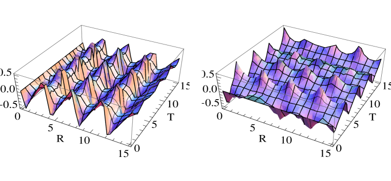
Figure 3: Behaviour of the energy density (left) and energy-flux (right), $\partial_{R}E,\partial_{T}E$, respectively, for the values of $\nu=0.13,\quad K=1$ and $\lambda=0.75$ of the time-dependent analogous of Pomeranski-Senkov black ring

IV Analytic continuation of the black ring with a single rotation

The line element of the black ring of Emparan-Reall can be obtained from (13) if $\nu=0$. In this case the polynomials $G(x)$ and $G(y)$ are of third order, and the roots are:

$$G(x)=\lambda(1-x)(x-(-1))(x-(-1/\lambda)).$$ (35)

Since $0<\lambda<1$, the root $x=-1/\lambda$ is not included in the range $-1\leq x\leq 1$. Following the above outlined method, the transformation $x\mapsto R$ is given by (handbook2 , p.219),

$$R = \int_{-1}^{x}{\frac{d{\tilde{x}}}{\sqrt{G({\tilde{x}})}}}$$

$$= \int_{-1}^{x}{\frac{d{\tilde{x}}}{\sqrt{\lambda(1-{\tilde{x}})({\tilde{x}}+1)({\tilde{x}}+1/\lambda)}}}$$

$$= \frac{2}{\sqrt{\lambda+1}}{\cal F}[\arcsin{\sqrt{\alpha}},\sqrt{p}],$$

$$\alpha = \frac{(\lambda+1)(1+x)}{2(\lambda x+1)},\quad p=\frac{2\lambda}{\lambda+1}.$$ (36)

For the variable $y$, the root $y=1$ is not included in the range $-\infty<y<-1$; then the interval for which $-G(y)>0$ is $-1/\lambda\leq y<-1$. Thus the transformation $y\mapsto\xi$ is given by:

$$\xi = \int_{-\frac{1}{\lambda}}^{y}{\frac{d{\tilde{y}}}{\sqrt{-G({\tilde{y}})}}}$$

$$= \int_{-\frac{1}{\lambda}}^{y}{\frac{d{\tilde{y}}}{\sqrt{\lambda(1-{\tilde{y}})(-1-{\tilde{y}})({\tilde{y}}+1/\lambda)}}}$$

$$= \frac{2}{\sqrt{\lambda+1}}{\cal F}[\arcsin{\sqrt{\delta}},\sqrt{m}],$$

$$\delta = \frac{(y\lambda+1)}{1-\lambda},\quad m=\frac{1-\lambda}{1+\lambda},$$ (37)

Again ${\cal F}$ is the incomplete elliptic integral of the first kind. The range of $\xi>0$ is $0<\xi<2{\cal K}\sqrt{1-\lambda}/(1+\lambda)$, where ${\cal K}$ is the Legendre’s complete integral of the first kind, ${\cal K}={\cal F}[\pi/2,k]$. Given $R(x)$ and $\xi(y)$, the inverse transformations are, according to the intervals of integration (see handbook2 , p. 837),

$$x(R) = \frac{-1-\lambda+2{}{\rm sn}^{2}(R,k)}{\lambda+1-(2\lambda){\rm sn}^{2}(R,k)},$$ (38)

$$y(\xi) = -\frac{1}{\lambda}+(\frac{1}{\lambda}-1){\rm sn}^{2}(\xi,k^{\prime})$$ (39)

$$k^{2} = \frac{2\lambda}{\lambda+1},\quad k^{\prime 2}=\frac{1-\lambda}{1+\lambda},$$ (40)

Performing now the complex transformation $\xi\mapsto iT$, and taking into account (29), we obtain

$$y(T)=-\frac{1}{\lambda}+(1-\frac{1}{\lambda})\frac{{\rm sn}^{2}(T,k)}{{\rm cn}^{2}(T,k)}.$$ (41)

This is a real function. The ranges of the new variables are $-\infty<R<\infty$ and $T$ is in principle $-\infty<T<\infty$ as well. However, $y(T)$ diverges whenever cn$(T,k)=0$, that is for $T=\pm(2n-1){\cal K},\quad n=1,2,\cdots$. The result of the double analytic continuation, $\xi\mapsto iT,\quad t\mapsto iz$ and $K\mapsto iK$, transforms the line element (13) with $\nu=0$ into

$$ds^{2} = -\frac{H(y)}{H(x)}(dz+\omega d\phi)^{2}-\frac{F(x,y)}{H(y)}d\phi^{2}$$ (42)

$$+\frac{F(y,x)}{H(y)}d\psi^{2}+\frac{2K^{2}H(x)}{(x-y)^{2}}(dR^{2}-dT^{2}),$$

where $x(R)$ and $y(T)$ are given by expressions (38) and (41), respectively. The metric function $J=0,$ while $\omega$, $G$, $H$ and $F$ are given as (Eqs. (14)-(15) with $\nu=0$)

$$\omega = -\frac{2K\lambda\sqrt{1-\lambda^{2}}}{H(y)}\frac{(1+\lambda)}{(1-\lambda)}(1+y),$$

$$G(x) = (1-x^{2})(1+\lambda x),$$

$$H(x) = 1+\lambda^{2}+2x\lambda,$$

$$F(x,y) = \frac{2K^{2}}{(x-y)^{2}}\{G(x)(1-y^{2})(1+\lambda y)(1-\lambda^{2})$$ (43)

$$+G(y)[2\lambda^{2}+x\lambda(1+\lambda^{2})+(x^{2}+x^{3}\lambda)(1-\lambda^{2})]\},$$

The signature of spacetime is not aparent from the expression (42). We have found out that the signs of the metric functions: $H(y(T))<0$, $H(x(R))>0$, $F(x(R),y(T))>0$, are independent of $\lambda$. On the other hand $F(y(T),x(R))>0$ if $\lambda>0.5$ and for other values of $\lambda$ the expression for $F$ does not have a definite sign. The term $[x(R)-y(T)]$ does not vanish anywhere therefore after the transformations, the metric remains regular.

The calculation of the element of the transitivity hypersurface gives in this case:

$${\rm det}\gamma_{ab} = g_{\psi\psi}(g_{zz}g_{\phi\phi}-g_{z\phi}^{2})$$ (44)

$$= \frac{F(x(R),y(T))F(y(T),x(R))}{H(y(T))H(x(R))},$$

IV.1 C-energy of the 5D polarized gravitational waves

We have evaluated numerically $\gamma_{\mu}\gamma^{\mu}$, the norm of the gradient of the transitivity surface, $\gamma_{\mu}=\partial_{\mu}\sqrt{{\rm det}\gamma_{ab}}$, with the result that it does not have a definite sign. Therefore, the spacetime again, should be interpreted as gravitational waves propagating in a cosmology. The energy of the system per unit Killing lenght $E$, can be calculated as the Brown-York energy Goncalves , Eq. (33), for the line element (42) gives

$$4E=1-\frac{(x(R)-y(T))}{\sqrt{2K^{2}H(x(R))}},$$ (45)

Since the functions $x(R)$ and $y(T)$ oscilate, $E$ has no clear limit at infinity, rather it oscillates all over the ranges of $R$ and $T$. The energy density and energy flux are given, respectively, by

$$E_{,R}=-\frac{1+\lambda^{2}+\lambda(x+y)}{4K(1+\lambda^{2}+2\lambda x)^{3/2}}x_{,R},\quad E_{,T}=-\frac{1}{4K\sqrt{2(1+\lambda^{2}+2\lambda x)}}y_{,T}.$$ (46)

From the previous expressions (plots in Fig. 4) we can clearly observe the tendency that as $K$ (previously interpreted as the rotation parameter of the ring and now stands for an extra polarization of the gravitational wave) gets larger, the energy does so too. Other interesting limiting situation is at $R=0,T=0$, that corresponds to a finite energy,

$$4E(R=0,T=0)=1-\frac{1}{\sqrt{2}k\lambda}.$$ (47)

Figure 4: Behaviour of the energy density (left) and energy-flux (right), $\partial_{R}E,\partial_{T}E$, respectively, for the time-dependent solution analogous to the black ring of Emparan-Reall. The values of the parameters are $\lambda=0.5$, $K=1$

V Conclusions

We note that the procedure of analytic continuation is not unique, therefore, it may be that the presented solutions are not the only solutions one is able to obtain by complexifying the black ring solutions.

The method presented to accomplish the complex analytic continuation works well for solutions of this kind, i.e. having in metric functions fourth or third degree polynomials, leads to real solutions in a analytically continued metric. However, interpretation turns out to be not a straight forward task, in that the coordinates transform into linear combinations of Jacobi functions that are periodic. In that sense the new coordinates $R,T$ should be compactified although the ranges are initially taken to be $(-\infty,\infty)$. The situation here reminds closed inhomogeneous cosmological models studied in Carmeli2 .

Curiously enough, the analytic continuation of the Myers and Perry solution has a well defined hypercylindrical regions where the gradient of the transitivity element is always positive. This has to do with the boost-symmetric structure of the spacetime. This does not happen in the other cases we have looked at, indicating that topologically these solutions have a complicated structure. It would be interesting to study the topology of these solutions in the future and to see as to whether one may impose special matching conditions as in Gowdy cosmologies Gowdy on the hypersurfaces of vanishing transitivity element gradient in order to cure some pathologies. Also would be interesting to study further the differences between the analytic continuations of the black holes vs the continuations of the black rings. It looks as though the solutions obtained from black holes have a superior asymptotic structure: due to their boost-rotational symmetry they inherit the future asymptotic structure of Minkowski space.

In the case of stationary generalizations of four-dimensional solutions one obtains a rich structure of singularities and event horizons. When these solutions are analytically continued into cylindrical and cosmological regions these structures are washed away. The $t=0$ singularities represent the inhomogeneous curvature singularity which is the source of the waves. The further evolution of the waves is conditioned by the overall metric expansion and is known to lead to a so-called Doroshkevich-Zeldovich-Novikov DZN universe Carmeli filled with non-interacting null fluids. Incidentally, one may perform a dimensional reduction of these solutions along the extra coordinate to obtain an inhomogeneous universe with a massless scalar field. These have a well-understood singularity structure: either they start with a strong curvature singularity, or present a Cauchy horizon similar to the Taub-NUT universe. The $r=0$ quasiregular singularity, on the other hand signals the presence of an angular deficit and is related to the C-energy function.

Finally, we have detected that the Pomeransky- Senkov solution is not well defined throughout all the original range $-1\leq x\leq 1$ and $-\infty<y<-1$, in the sense that metric functions (for instance, $H(x,y)$) changes sign and has zeroes besides the zeros considered as horizons; this makes problematic the interpretation once the analytic continuation has been performed and restricts the range of the aplicability of the method.

References

• (1) O. Aharony, M. Fabinger, G. T. Horowitz and E. Silverstein, Clean Time-dependent String Backgrounds from Bubble Baths, JHEP, 0207 (2002)007, arXiv: hep-th/0204158.
• (2) E. Witten, Nucl. Phys. B 195, 481 (1982)
• (3) F. Dowker, J. P. Gauntlett, G. W. Gibbons and G. T. Horowitz, Phys. Rev. D 53, 7115 (1996). hep-th/9512154
• (4) G. T. Horowitz and R. C. Myers, Phys. Rev. D 59, 026005 (1999). hep-th/9008079
• (5) D. Ida, T. Shiromizu and H. Ochiai, Phys. Rev. D 65, 023504 (2002). hep-th/0108056
• (6) M. Costa and M. Gutperle, JHEP 0103, 027 (2001), hep-th/0012072; M. Fabinger and P. Horava, Nucl. Phys. B580, 243 (2000). hep-th/0002073.
• (7) T.Piran, P.N. Safier and J. Katz, Phys. Rev. D 34, 331 (1986); T. Piran, P.N. Safier, R. F. Stark, General numerical solution of cylindrical gravitational waves, Phys. Rev. D 32, 3101 (1985).
• (8) M. Carmeli, Ch. Charach and S. Malin, Survey of cosmological models with gravitational, scalar and electromagnetic waves, Phys. Rep. 76, 79 (1981). M. Carmeli and Ch. Charach, The Einstein-Rosen Gravitational waves and cosmology, Found. of Physics 14, 963 (1984)
• (9) A. Feinstein and J. Ibáñez, Phys. Rev. D 39, 470 (1989)
• (10) R. C. Myers, H. S. Perry, Black holes in higher Dimensional Space-Times, Ann. Phys. 172, 304 (1986).
• (11) T. Harmark, Phys. Rev. D 70, 124002 (2004); T. Harmark and P. Olesen, Phys. Rev. D 72, 124017 (2005).
• (12) J. M. M. Senovilla, Trapped surfaces, horizons and exact solutions in higher dimensions, Class. Quant. Grav. 19, L113 (2002).
• (13) C.W. Misner, J.Math.Phys.4, 924 (1963)
• (14) S. M. C. V. Goncalves, Unpolarized radiative cylindrical spacetimes: trapped surfaces and quasilocal energy, Class. Quantum Grav. 20, 37 (2003).
• (15) J. Bičak and B.Schmidt, Phys. Rev. D 40, 1827 (1989)
• (16) R. Gowdy, Phys. Rev. D 75, 084011 (2007);
• (17) A. A. Pomeransky and R. A. Sen’kov: Black ring with two angular momenta arXiv: hep-th/0612005;
• (18) H. Elvang, M. J. Rodríguez: Bicycling black rings, JHEP 04(2008)045.
• (19) R. Emparan and H. S. Reall, Phys. Rev. Lett. 88, 101101 (2002); R. Emparan and H. S. Reall, Phys. Rev. D 65, 084025 (2002).
• (20) G. A. Korn and T. M. Korn, Mathematical Handbook for Scientists and Engineers, (Mc Graw-Hill, New York, 1968), Chap. 21.
• (21) I. S. Gradshteyn and I. M. Ryzhik, Table of Integrals, Series, and Products, (Academic Press, N.Y. 1980)
• (22) M. Carmeli, Ch. Charach and A. Feinstein, Ann. Phys. (N.Y.) 150,392 (1983)
• (23) R. Gowdy, Phys. Rev. Lett. 27, 827, (1971)