SQUID Detection of Quantized Mechanical Motion

Abstract

We predict that quantized mechanical motion can be detected by embedding a mechanical resonator into a quantum SQUID. If the system is tuned to the regime when a plasma frequency of the SQUID matches the resonator frequency, the doubly-degenerate quantum level of the system is split by the coupling between the SQUID and the resonator. Observation of an avoided crossing as the function of external flux would be an unambiguous evidence of quantum nature of mechanical motion. We also investigate the conditions maximizing the level splitting.

The interest in nanoelectromechanical systems (NEMS) has been growing rapidly Cleland ; Blencowe04 because of their wide range of potential technological applications in detection and sensing, and their importance in testing fundamentals of quantum theory. The possibility to observe quantum mechanical motion of an oscillator has important implications in the understanding to which extent macroscopic objects obey the laws of quantum mechanics Leggett02 . NEMS can play also an important role in quantum computation where they have been proposed as qubits Savel'ev06 , memory elements Cleland04 ; Pritchett , and quantum buses Cleland04 ; Zou04 . Coupling of nanomechanical oscillators to a qubit has been also thoroughly investigated in the literature and many schemes of this kind have been proposed with Cooper-pair boxes Armour02 ; Martin04 ; Rabl04 ; Wei06 ; Armour08 ; Hauss08 , Josephson junctions (phase qubits) Cleland04 ; Trees07 , quantum point contacts Ruskov05 , and quantum dotsLiao08 . Recently the dispersive coupling of a NEMS to a Cooper-pair box has been realized LaHaye09 .

Coupling of nanomechanical oscillators to SQUIDs has been recently intensively investigated Zhou06 ; Buks06 ; Xue07 ; Wang08 ; Zhang09 ; Pugnetti09b . The high sensitivity of SQUIDs to tiny changes in the magnetic flux has suggested that the position of a nanomechanical resonator could be monitored by integrating the oscillator into the superconducting loop of a dc SQUID; indeed the transport properties of this superconducting circuit in presence of a uniform magnetic field depend on the position of the oscillator, since this position modifies the total area threaded by the flux. Recently this scheme has been demonstrated for the detection of the thermal motion of a mechanical resonator in the classical regime Etaki08 . Due to the high degree of control achieved on quantum SQUIDs, coupling nanomechanical resonators to SQUIDs is a promising scheme for observing quantum effects in the motion of these oscillators as well.

In this Article, we develop a protocol of detecting quantized mechanical oscillations with a SQUID coupled to a mechanical resonator. We show that the signature of this quantized motion is a splitting of an energy level associated with the SQUID due to the coupling to a resonator. In the case of resonant coupling, this splitting can be detected by standard techniques developed for flux qubits Mooij99 . We stress that achieving this regime is not straightforward as the typical frequencies of the SQUID (of the order of few GHz) and the oscillator (MHz range) do not naturally match to allow for a resonant behavior. In this Article we show that this is however possible by tuning the external magnetic field and the bias current with available experimental setups.

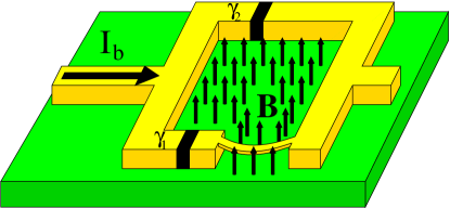
Figure 1: A sketch of the device we study: one arm of a dc SQUID is free to oscillate in the plane of the SQUID itself. A uniform magnetic field $B$ orthogonal to the SQUID plane is present and a dc bias current $I_{b}$ flows through the device. The two Josephson junctions, whose phase drops are respectively $\gamma_{1}$ and $\gamma_{2}$, are taken to be identical.

The system we consider is schematically drawn in Fig. 1. A dc SQUID is made of a superconducting loop of total area $A$ with an arm of length $l$ that can oscillate freely in the plane of the loop. For simplicity we assume that only a single mode of oscillation with the frequency $\omega$ can be excited. This mode is described by the dynamical variable $X$ representing the shift of the center-of-mass of the resonator (with the mass $m$) with respect to its rest position. The quantum effects related to mechanical motion of this oscillator appear at the scale of the amplitude of zero-point motion $X_{0}=\sqrt{\hbar/2m\omega}$. The SQUID further comprises two Josephson junctions of equal critical currents $I_{c}$ and shunting capacitances $C$; the typical energy scales related to the physics of the junctions are the Josephson energy $E_{J}=\hbar I_{c}/2e$ and the charging energy $E_{c}=(2e)^{2}/2C\ll E_{J}$, whose magnitude depends on the geometry of the junctions. The typical time scale for the dynamics of the junctions is set by the inverse plasma frequency $\omega_{\mathrm{pl}}=\sqrt{2E_{J}E_{c}}/\hbar$. The dynamics of the SQUID is described by the two gauge-invariant phase drops $\gamma_{1}$ and $\gamma_{2}$ across the two junctions.

The coupling of the SQUID dynamics to mechanical motion is provided by the position dependence of the magnetic flux threading the SQUID loop. The two phases are constrained by the requirement that the superconducting order parameter is single valued,

$$\gamma_{1}-\gamma_{2}=2\pi\left(\frac{\Phi}{\Phi_{0}}+n\right)\,,$$ (1)

where $\Phi_{0}=h/2e$ is the flux quantum; the total flux $\Phi$ is the sum of three contributions. The first one comes from the external bias $\Phi_{e}=BA\equiv\Phi_{0}\phi_{e}$, while the second one $\Phi_{m}=BlX$ depends on the position of the mechanical resonator and provides the coupling between the mechanical resonator and the SQUID. If the circuit also has non-negligible self inductance $L$, the third contribution to the total flux $\Phi$ comes from the current circulating in the loop; if $I_{1}$ and $I_{2}$ are the currents flowing through each junction, the self-induced flux reads $L(I_{1}-I_{2})/2$. This device has three degrees of freedom; if $L=0$, then the constraint expressed by Eq. (1) reduces the number of degrees of freedom from three to two. In the following, we assume that the dissipation effects are negligible.

Quantum coherence in the motion of the mechanical resonator can be detected via spectroscopic measurements on the quantum SQUID. Indeed, the energy levels associated with the SQUID degrees of freedom are shifted due to the coupling to the oscillator. However, this shift is of the second order in the coupling and for realistic experimental parameters is very small. We employ therefore below a different scheme, which provides the result which is of the first order in the coupling. One first chooses an appropriate set of values for the externally controllable quantities $I_{b}$ and $\Phi_{e}$ such that the system can be trapped in a minimum in which one of the eigenfrequencies of the electromagnetic modes is the same as the frequency of mechanical oscillations (to be referred below as degeneracy condition); then one moves slightly away from this degeneracy condition by changing the remaining external parameter. A plot of the energy levels as functions of the external parameters should display an avoided level crossing, which is a clear indication that the SQUID is coupled to a coherent quantum system.

It is useful to describe the system in terms of three dimensionless variables $\gamma=(\gamma_{1}+\gamma_{2})/2$, $\phi=\Phi/\Phi_{0}$ and $\xi=BlX/\Phi_{0}$. The potential energy of the system reads

$$\begin{split}U=E_{J}&\left[-2\cos\gamma\cos(\pi\phi)-\frac{I_{b}}{I_{c}}\gamma-\pi\frac{I_{b}}{I_{c}}\xi+\frac{\xi^{2}}{2\mathscr{A}^{2}}+\right.\\ &\left.\quad+\frac{2\pi}{\beta_{L}}(\phi-\xi-\phi_{e})^{2}\right],\end{split}$$ (2)

where we have introduced the parameters

$$\mathscr{A}=\sqrt{\frac{2E_{J}}{\hbar\omega}}\frac{BlX_{0}}{\Phi_{0}}\,;\ \beta_{L}=\frac{2LI_{c}}{\Phi_{0}}\ .$$ (3)

The parameter $\mathscr{A}$ is proportional to the flux threading the area swept by the mechanical resonator and plays the role of a coupling parameter, as we show below. Typical values of $\mathscr{A}=4\times 10^{-5}$ can be obtained assuming $I_{c}=1\mu$A, $\omega=1$GHz, $l=1\mu$m, $X_{0}=10$fm and $B=0.1$T. When the temperature is low enough for the system to reach the quantum regime, the coordinates typically oscillate around a minimum of the potential corresponding to the values $\bar{\gamma}$, $\bar{\phi}$ and $\bar{\xi}$. We can approximate the dynamics as a three-dimensional harmonic oscillator, with the energy being a quadratic form,

$$\begin{split}E_{\mathrm{tot}}=\sum_{i}&\frac{\hbar^{2}}{2E_{c}}\dot{q}_{i}^{2}+\sum_{i,j}E_{J}V_{ij}q_{i}q_{j}\ ,\end{split}$$ (4)

where the coordinates $q_{i}$ read

$$q_{1}=\gamma-\bar{\gamma};\ q_{2}=\pi(\phi-\bar{\phi});\ q_{3}=\dfrac{1}{\Omega}\dfrac{1}{\sqrt{2}\mathscr{A}}(\xi-\bar{\xi})\,,$$ (5)

and

$$V=\left(\begin{array}[]{@{}ccc@{}}r&-s&0\\ -s&r+\dfrac{2}{\pi\beta_{L}}&-\dfrac{2\sqrt{2}\mathscr{A}}{\beta_{L}}\Omega\\ 0&-\dfrac{2\sqrt{2}\mathscr{A}}{\beta_{L}}\Omega&\left(1+\dfrac{4\pi\mathscr{A}^{2}}{\beta_{L}}\right)\Omega^{2}\end{array}\right)\,.$$ (6)

(We have introduced $r=\cos\bar{\gamma}\cos(\pi\bar{\phi})$, $s=\sin\bar{\gamma}\sin(\pi\bar{\phi})$ and $\Omega=\omega/\omega_{\mathrm{pl}}$). The coupling $V_{23}$ between the mechanical resonator and the SQUID is proportional to the ratio $\mathscr{A}/\beta_{L}$ (for devices with a low self-inductance this behavior no longer holds, see below for discussion); the decoupled regime can be obtained for either $B\to 0$ or $L\to\infty$. The coordinate $Q_{1}=\gamma-\bar{\gamma}$, corresponding to one of the electromagnetic degrees of freedom, oscillates with the frequency $\omega_{\mathrm{pl}}\sqrt{\cos\bar{\gamma}\cos(\pi\bar{\phi})}$; therefore if a minimum $(\bar{\gamma},\bar{\phi},\bar{\xi})$ is such that

$$\cos\bar{\gamma}\cos(\pi\bar{\phi})=\Omega^{2}\,,$$ (7)

the frequencies associated with the motion of average phase drop $\gamma$ and oscillator motion coincide up to correction of second order in $\mathscr{A}$; we show below that the equality is indeed exact to all orders in the coupling. Since in the low-inductance limit the coordinates $\phi$ and $\xi$ are not independent, it is convenient to switch to the basis where the submatrix corresponding to $\xi$ and $\phi$ is diagonalized. The analytic expression for the matrix in the new basis is quite cumbersome; below we give this expression in the limit in which the degeneracy condition (7) holds,

$$V^{\prime}=\left(\begin{array}[]{@{}ccc@{}}\Omega^{2}&-s\dfrac{\sqrt{2}\pi\mathscr{A}}{C}\Omega&\dfrac{s}{C}\\ -s\dfrac{\sqrt{2}\pi\mathscr{A}}{C}\Omega&\Omega^{2}&0\\ \dfrac{s}{C}&0&\Omega^{2}+\dfrac{2C^{2}}{\pi\beta_{L}}\end{array}\right)\ ,$$ (8)

with $C=\sqrt{2\pi^{2}\mathscr{A}^{2}\Omega^{2}+1}$. The first and second row and column correspond to the phase drop $\gamma$ and to the mechanical degree of freedom, respectively. The parameters $I_{b}$ and $\Phi_{e}$ corresponding to the degeneracy condition are found if one solves the equation set,

$$\left\{\begin{array}[]{l}I_{b}/I_{c}=2\sin\bar{\gamma}\cos(\pi\bar{\phi})\\ 2\beta_{L}^{-1}(\bar{\phi}-\phi_{e}-\bar{\xi})=-\cos\bar{\gamma}\sin(\pi\bar{\phi})\\ \bar{\xi}=4\pi\mathscr{A}^{2}\beta_{L}^{-1}\left(\bar{\phi}-\phi_{e}-\bar{\xi}+(\beta_{L}I_{b})/(4I_{c})\right)\\ \cos\bar{\gamma}\cos(\pi\bar{\phi})=\Omega^{2}\,,\end{array}\right.$$ (9)

where the first three lines are satisfied by stationary points of the potential energy (2) and the fourth line is the degeneracy condition. In a minimum one must have $V>0$. The unknowns are the coordinates $(\bar{\gamma},\bar{\phi},\bar{\xi})$ of the minimum and $\Phi_{e}$; we use $I_{b}$ to tune the system to the degeneracy pointfoot1 .

Next, we quantize the system. The Hamiltonian reads

$$H=\sum_{i=1}^{3}\hbar\omega_{i}a_{i}^{\dagger}a_{i}+\sum_{i\neq j}\dfrac{1}{4}\hbar\omega_{\mathrm{pl}}\dfrac{\omega_{\mathrm{pl}}}{\sqrt{\omega_{i}\omega_{j}}}V^{\prime}_{ij}(a_{i}^{\dagger}+a_{i})(a_{j}^{\dagger}+a_{j})$$ (10)

with $\omega_{i}=\omega_{\mathrm{pl}}\sqrt{V^{\prime}_{ii}}$. When the condition (7) is fulfilled, the first excited levels $|100\rangle$ and $|010\rangle$ are quasi-degenerate and the Hamiltonian (10) restricted to their subspace becomes

$$H=\left(\begin{array}[]{@{}cc@{}}\hbar\omega&\lambda\\ \lambda&\hbar\omega\end{array}\right)\,,\ \ \lambda=\dfrac{1}{4}\hbar\omega_{\mathrm{pl}}\dfrac{1}{\Omega}V^{\prime}_{\xi\gamma}\,.$$ (11)

Fig. 2 shows the dependence of the dimensionless level splitting $\lambda/\hbar\omega_{\mathrm{pl}}$ on the dimensionless external flux $\phi_{e}$.

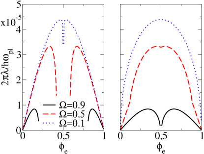
Figure 2: Dimensionless splitting $\lambda/\hbar\omega_{\mathrm{pl}}$ versus the external flux $\phi_{e}$ for the coupling parameter $\mathscr{A}=4\times 10^{-5}$. The self-inductance parameter $\beta_{L}$ is $10^{-4}$ for the left panel and $1$ for the right panel. Dotted, dashed, and solid lines correspond to $\Omega=\omega/\omega_{\mathrm{pl}}=0.1,0.5$ and $0.9$, respectively. The plots are periodic, the period being one flux quantum.

The maximum level splitting is obtained for a specific value of the external flux and depends very weakly on the loop self-inductance; however the value of the flux at which the maximum is achieved, does; see below for further discussion. The magnitude of the splitting is of the order of $10^{-5}\hbar\omega_{\mathrm{pl}}$. The value of the ratio $\Omega=\omega/\omega_{\mathrm{pl}}$ plays an important role: lower values correspond to bigger maximum splittings and are thus preferable.

To enable the detection, the potential well formed at the chosen minimum must be capable of containing quantum states. The number of bound states can be estimated by the ratio between the energy difference $\Delta U$ between the minimum and the closest saddle point and the energy level separation, which is roughly $\hbar\omega$,

$$\dfrac{\Delta U}{\hbar\omega}=\dfrac{\Delta U}{E_{J}}\dfrac{1}{\Omega}\sqrt{\dfrac{E_{J}}{2E_{c}}}\equiv\Delta u\sqrt{\dfrac{E_{J}}{2E_{c}}}\,.$$ (12)

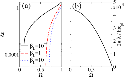
Figure 3: (a) the dimensionless depth $\Delta u$ of the minimum featuring maximum splitting $\lambda$ is plotted as a function of the ratio $\Omega=\omega/\omega_{\mathrm{pl}}$, for different values of the self-inductance parameter: $\beta_{L}=10^{-4}$ (solid line), $\beta_{L}=1$ (dashed line) and $\beta_{L}=10$ (dotted line). (b) the maximum value of the dimensionless splitting $\lambda/\hbar\omega_{\mathrm{pl}}$ is plotted as a function of $\Omega$; here $\beta_{L}=1$, but the result is independent of $\beta_{L}$.

Fig. 3a displays plots of the quantity $\Delta u$, defined by Eq. (12), as a function of $\Omega$ for different values of the self-inductance parameter $\beta_{L}$; one sees that small values of $\Omega$ correspond to very shallow minima in the potential energy, whereas the deepest minima correspond to devices in which $\omega=\omega_{\mathrm{pl}}$. However Fig. 3b shows that for these devices no gap is expected in the first order in the coupling; this rather surprising fact can be further illustrated by considering the dependence of the matrix element $V^{\prime}_{\gamma\xi}$ on $s=\sin\gamma\sin(\pi\phi)$ in Eq. (8): for $\Omega=1$, one has $\cos\gamma\cos(\pi\phi)=0$ and thus $s=0=\lambda$. Because of this trade-off, the optimal condition corresponds to an intermediate case. Note however that $\Delta u$ depends on $E_{J}$ and $E_{c}$ only via the ratios $\Omega=\omega/\omega_{\mathrm{pl}}$ and $I_{b}/I_{c}$ and thus can be tuned independently of $E_{J}/E_{c}$. Therefore a bigger minimum depth can be obtained by designing the SQUID so that the ratio $E_{J}/E_{c}$ is large.

We now comment on the role of the self-inductance. The curve in Fig. 3b is very little affected by the value of $\beta_{L}$, implying that this parameter is not relevant for improving the splitting $\lambda$; on the contrary, the curves in Fig. 3a show that the dimensionless depth $\Delta u$ of the minimum well is drastically reduced by increasing the self-inductance of the loop. Thus loops of smaller self-inductance are preferable.

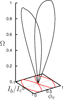
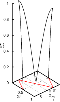
Figure 4: Plots of the solutions of Eqs. (9) giving maximum value of the dimensionless splitting $\lambda/\hbar\omega_{\mathrm{pl}}$; left panel $(I_{b}/I_{c},\phi_{e},\Omega)$, right panel $(\phi,\gamma,\Omega)$. A projection of the points onto to the horizontal plane is also displayed for reader’s convenience.

Finally, Fig. 4 represents numerical solutions of Eqs. (9) used in the previous figures. The right panel shows the values of the dimensionless external parameters $I_{b}/I_{c}$ and $\phi_{e}$ that corresponds to the maximum value of the gap $\lambda$ for values of $\Omega$ between 0 and 1, while the left panel shows a plot of the coordinates $(\bar{\gamma},\bar{\phi})$ of the best minimum. As expected, the results are symmetric with respect to simultaneous current inversion $I_{b}\to-I_{b}$ and flux reflection $\phi_{e}\to 1-\phi_{e}$; this can be seen from Eqs. (9), where in this case if $(\gamma,\phi,\xi,I_{b}/I_{c})$ is a solution, then also $(\pi-\gamma,1-\phi,-\xi,-I_{b}/I_{c})$ solves the equations.

In conclusion, we found that quantum oscillations of a NEMS embedded into a SQUID can be detected by spectroscopic measurements in the regime when one of the plasma frequencies of the SQUID matches the frequency of the mechanical resonator. This frequency matching is possible with the current experimental techniques, and the scheme has two parameters (external flux and external current) to simultaneously tune the system to the vicinity of the degeneracy point and perform spectroscopic measurements around this point. Measurements of splitting of the degenerate doublet state displaying an avoided crossing would be an unambiguous evidence of quantum nature of mechanical vibrations.

We acknowledge the financial support of the Future and Emerging Technologies programme of the European Commission, under the FET-Open project QNEMS (233992). We thank Herre van der Zant, Samir Etaki, and Menno Poot for useful discussions.

References

- (1) A. N. Cleland, Fundations of Nanomechanics, Springer, Berlin (2003).
- (2) M. Blencowe, Phys. Rep. 395, 159 (2004).
- (3) A. J. Leggett, J. Phys: Condensed Matter 14, R415 (2002).
- (4) S. Savel’ev, X. Hu, and F. Nori, New J. Phys. 8, 105 (2006).
- (5) A. N. Cleland and M. R. Geller, Phys. Rev. Lett. 93, 070501 (2004); M. R. Geller and A. N. Cleland, Phys. Rev. A 71, 032311 (2005);
- (6) E. J. Pritchett and M. R. Geller, Phys. Rev. A 72, 010301 (2005).
- (7) X. B. Zou and W. Mathis, Phys. Lett. A 324, 484 (2004).
- (8) A. D. Armour, M. P. Blencowe, and K. C. Schwab, Phys. Rev. Lett. 88, 148301 (2002).
- (9) I. Martin et al, Phys. Rev. B 69, 125339 (2004).
- (10) P. Rabl, A. Shnirman, and P. Zoller, Phys. Rev. B 70, 205304 (2004).
- (11) L. F. Wei em et al, Phys. Rev. Lett. 97, 237201 (2006).
- (12) A. D. Armour and M. P. Blencowe, New J. Phys. 10, 095004 (2008).
- (13) J. Hauss et al, New J. Phys. 10, 095018 (2008).
- (14) B. R. Trees et al, Phys. Rev. B. 76, 224513 (2007); J. Wabnig, J. Rammer, and A. L. Shelankov, ibid 75, 205319 (2007).
- (15) R. Ruskov, K. Schwab, and A. N. Korotkov, Phys. Rev. B 71, 235407 (2005).
- (16) J. Q. Liao and L. M. Kuang, Eur. Phys. J. B 63, 79 (2008).
- (17) M. D. LaHaye et al, Nature 459, 960 (2009).
- (18) X. Zhou and A. Mizel, Phys. Rev. Lett. 97, 267201 (2006).
- (19) E. Buks and M. P. Blencowe, Phys. Rev. B 74, 174504 (2006).
- (20) F. Xue et al, Phys. Rev. B 76, 064305 (2007).
- (21) Y.-D. Wang, K. Semba, and H. Yamaguchi, New J. Phys. 10, 043015 (2008).
- (22) J. Zhang, Y. X. Liu, and F. Nori, Phys. Rev. A 79, 052102 (2009).
- (23) S. Pugnetti et al, Phys. Rev. B 79, 174516 (2009).
- (24) S. Etaki et al, Nature Phys. 4, 785 (2008).
- (25) J. E. Mooij et al, Science 285, 1036 (1999).
- (26) In principle one, many or no solutions can exist for a particular set of parameters; when more then one solution exist, we take the one with the bigger gap .