Higher order approximation of isochrons

Abstract

Phase reduction is a commonly used techinque for analyzing stable oscillators, particularly in studies concerning synchronization and phase lock of a network of oscillators. In a widely used numerical approach for obtaining phase reduction of a single oscillator, one needs to obtain the gradient of the phase function, which essentially provides a linear approximation of isochrons. In this paper, we extend the method for obtaining partial derivatives of the phase function to arbitrary order, providing higher order approximations of isochrons. In particular, our method in order $2$ can be applied to the study of dynamics of a stable oscillator subjected to stochastic perturbations, a topic that will be discussed in a future paper. We use the Stuart-Landau oscillator to illustrate the method in order $2$.

1 Introduction and statement of main results

Weak perturbations of limit cycle oscillators are of great interest in a variety of fields in physics, chemistry, engineering, and quantitative biology, whenever the system under study displays stable oscillations. A powerful theoretical approach in the analysis of weakly perturbed limit cycles, particularly in relation to synchronization and phase lock of a network of oscillators, is to reduce the description of the system to a single “phase” variable. This phase reduction procedure is the focus of the present paper.

In this introduction, we begin by describing a standard numerical approach for obtaining first order phase reduction, due to I.G. Malkin [11, 12]. We then explain our higher order method, which is summarized in Theorem 1.1, and illustrate it in order $2$ using the well-known Stuart-Landau oscillator as an example. Proofs are are given in the subsequent sections. Our focus is on the theoretical underpinnings of the method rather than on the details of numerical implementation, but we provide a numerical example to illustrate the approach.

The following set-up is assumed to hold throughout. Let $F$ be a smooth (i.e., continuously differentiable to all orders) vector field on $n$-dimensional Euclidean space $\mathbb{R}^{n}$. The flow line of an initial point $x$ will be denoted $\phi_{t}(x)$, or simply $x(t)$, for $t\in\mathbb{R}$. Let $\mathcal{C}$ be a stable (hyperbolic) limit cycle of the differential equation $\dot{x}=F(x)$ having period $T>0$. We write $\omega=1/T$ for the reciprocal of the period. The stability condition means that for any given point $x$ on $\mathcal{C}$, there exists a linear $n-1$-dimensional subspace $W(x)$ in $\mathbb{R}^{n}$ transverse to $F(x)$ such that vectors in $W(x)$ contract exponentially under positive iterations of the differential $(d\phi_{T})_{x}$ of the flow map at $x$. That is, $|(d\phi_{T})^{n}v|<C\lambda^{n}|v|$ for positive constants $C$, $\lambda<1$, positive integer $n$, and all $v$ in $W(x)$. As we are only concerned with the system near $\mathcal{C}$, there is no loss of generality in assuming that $F$ is a complete vector field, so that the flow lines $\phi_{t}(x)$ are defined for all $t\in\mathbb{R}$ and all $x\in\mathbb{R}^{n}$.

1.1 The phase function

We briefly review a few well-known facts about the dynamics near a stable limit cycle for the purpose of setting up notation.

Due to normal hyperbolicity on $\mathcal{C}$, it is known [6] that a neighborhood of the limit cycle is continuously foliated by contracting manifolds, $\mathcal{W}(x)$, for each $x\in\mathcal{C}$, where the $\mathcal{W}(x)$ are smooth submanifolds tangent to $W(x)$ at $x$ and diffeomorphic to an open disc. The foliation is invariant, i.e., $\phi_{t}$ maps $\mathcal{W}(x)$ into $\mathcal{W}(\phi_{t}(x))$ for all $t\geq 0$ and all $x$ in $\mathcal{C}$. Furthermore, the foliation is smooth since $\mathcal{C}$ is an orbit of a smooth flow. In fact, we can use maps of the form $H(z,t)=\varphi_{t}(z)$, where $z\in\mathcal{W}(x)$ and $t\in(-a,a)$, to produce smooth foliation charts around $x$.

Let $\Theta$ be a function defined on a sufficiently small neighborhood of $\mathcal{C}$, whose level sets are the local contracting manifolds and such that $\Theta(x(t))=\omega t$ modulo integer translations. I.e., $\Theta$ takes values in $\mathbb{R}/\mathbb{Z}$. We often regard $\Theta$ simply as a function into $\mathbb{R}$, keeping in mind that, in this case, $\Theta(x(t+nT))=\Theta(x(t))+n$. Derivatives of $\Theta$, on the other hand, are single-valued functions into $\mathbb{R}$.

We refer to $\Theta$ as the phase function of the oscillator. It is, thus, a smooth function on some neighborhood of the limit cycle such that $\Theta(y)=\Theta(x)$ iff $|\phi_{t}(y)-\phi_{t}(x)|\to 0$ as $t\to\infty$ whenever $x\in\mathcal{C}$ and y lies in a sufficiently small neighborhood of $\mathcal{C}$.

The level sets of $\Theta$ are also called isochrons [18]. The existence of isochrons was first proved in [4]. Since the component functions of the gradient of $\Theta$ give the change in phase due to a small change in the respective position coordinates [1], the graphs of those functions are often referred to as phase response curves. This notion is widely used in theoretical and experimental neuroscience. For example, some theoretical studies have examined how the shape of the phase response curves affect the sychronization dynamics of coupled oscillators [5, 2]. Other studies have investigated the connection between phase response curves and mechanisms of brain function and pathology such as autoassociative memory [10] and epileptic seizures [15]. The phase response curves of neurons in the neocortex have been experimentally determined [13, 16].

1.2 First order phase reduction

Before explaining our main results, which are collected in Theorem 1.1, it is useful to briefly review the standard method of phase reduction. For a more complete discussion the reader is referred to [8], Chapter 10, and to [1].

It is easy to see why the derivatives of $\Theta$ are needed when studying weak perturbations of a stable oscillator described by $\dot{x}=F(x)$. Let such a perturbation be given by the new equation $\dot{x}=F(x)+\epsilon G(x,t)$, where $\epsilon$ is a small positive number. Then

$$\frac{d}{dt}\Theta(x(t))={\nabla}\Theta(x(t))\cdot\dot{x}=\omega+\epsilon{\nabla}\Theta(x(t))\cdot G(x,t)$$ (1)

where ${\nabla}\Theta$ is the gradient of the phase function. Writing $Q^{(1)}_{t}={\nabla}\Theta(x_{0}(t))$, where $x_{0}(t)$ is the point on the limit cycle on the same isochron as $x(t)$, then

$$\frac{d\Theta}{dt}=\omega+\epsilon Q^{(1)}_{t}\cdot G(x_{0}(t),t)+\epsilon\mathcal{O}(|x(t)-x_{0}(t)|).$$ (2)

One then proceeds by discarding the term $\epsilon\mathcal{O}(|x(t)-x_{0}(t)|)$ and analyzing the resulting system. Thus implementing the phase reduction method in order $1$ in $|x(t)-x_{0}(t)|$ requires finding the gradient of the phase function along the limit cycle of the unperturbed oscillator, denoted by $Q^{(1)}_{t}$ in the last equation.

One practical method for obtaining the gradient of $\Theta$ is by solving the equation:

$$\dot{Q}^{(1)}_{t}+DF^{\dagger}(x_{0}(t))Q^{(1)}_{t}=0$$ (3)

where the dot indicates time derivative and $DF^{\dagger}(x_{0}(t))$ is the transpose of the Jacobian matrix of $F$ evaluated along the limit cycle. This procedure was suggested by Malkin [7, 11, 12] and later by others independently [14, 3]. The reader is referred to [7], Chapter 9, for more details of the Malkin’s theorem and [8], Chapter 10 for a historical note on phase reduction. One can find $Q^{(1)}_{t}$ by numerically integrating the equation backwards in time for any initial condition satisfying $Q_{0}^{(1)}\cdot F(x_{0}(0))=1$, over an interval of time long enough to allow the solution to stabilize to a periodic one [17].

One limitation of the method as presented above is that it is only valid to first order. To develop higher order phase reduction, it is necessary to obtain higher order partial derivatives of $\Theta$. However, to the best of our knowledge, an approach to higher order approximations of $\Theta$ similar in spirit to the above due to Malkin for finding the gradient of $\Theta$ has not been described so far in the literature. The goal of the present paper is to develop a numerical method to obtain partial derivatives of $\Theta$ to arbitrary order.

Even within the framework of first order phase reduction (i.e. Equation (2)), in certain situations, as when dealing with weak stochastic perturbations of oscillators, one may need to know the derivatives of $\Theta$ along the limit cycle to orders greater than $1$. For example, in [19], a stochastic version of phase reduction is given using the 2nd order partial derivatives of $\Theta$ to obtain the mean and variance of the period of a limit cycle oscillator. They apply their results to the Stuart-Landau oscillator, for which an explicit form of $\Theta$ can be obtained analytically. In general, however, an analytical form of $\Theta$ is not available. Therefore, the method we present here is of particular interest in order two for studying the dynamics of a limit cycle oscillator subjected to stochastic perturbations. This will be discussed in detail in a future paper.

The main result of this paper, which is described in Theorem 1.1 below, amounts to a recursive procedure for finding the higher order derivatives of $\Theta$ in which the first step is Malkin’s method just described.

1.3 The main result

We need a few definitions first. Let $v=(v_{1},\dots,v_{n})$ be any vector in $\mathbb{R}^{n}$ and $f$ any differentiable real-valued function in $x_{1},\dots,x_{n}$. Given a multi-index $J=(j_{1},\dots,j_{n})$, i.e., an $n$-dimensional vector with non-negative integer entries, we write $v^{J}=v_{j_{1}}\dots v_{j_{n}}$ and $f_{J}=D^{J}f=D_{1}^{j_{1}}\dots D_{n}^{j_{n}}f$, where $D_{i}$ denotes partial derivative with respect to $x_{i}$ and $D_{i}^{k}=D_{i}\dots D_{i}$ ($k$ times). Let $f^{(k)}$ represent the symmetric $k$-multilinear map on $\mathbb{R}^{n}$ characterized (via polarization of polynomial maps) by

$$f^{(k)}(v,\dots,v)=\sum_{|J|=k}f_{J}v^{J}$$

for all $v\in\mathbb{R}^{n}$. The sum is over all multi-indices $J$ of order $|J|=j_{1}+\dots+j_{n}=k$. Here, and often later, we omit reference to the point $x$ where the derivatives are taken. When necessary, this point is indicated as a sub-index; thus $f_{x}^{(2)}(v,w)$ is the bilinear map evaluated at the vectors $v,w$ regarded as tangent vectors at $x\in\mathbb{R}^{n}$, where $x$ is the point where the partial derivatives of $f$ are calculated.

We now define

$$Q_{t}^{(k)}=\Theta^{(k)}_{\phi_{t}(x)},$$ (4)

for some fixed $x\in\mathbb{R}^{n}$, where $\phi_{t}$ is the flow of $F$. Similarly, we define $F^{(k)}$, which is now a vector valued, symmetric, $k$-multilinear map. (A convenient alternative description of $\Theta^{(k)}$ and $F^{(k)}$, and more generally of the higher order derivative forms associated to tensor fields, will be given later in the paper.) In particular, $F^{(1)}$ is the linear map which to $v\in\mathbb{R}^{n}$ gives the directional derivative of $F$ along $v$, i.e., $F^{(1)}(v)=D_{v}F=\sum_{j}v_{j}D_{j}F$, where $D_{v}F$ is defined by this identity.

Another general concept needed below is the symmetric composition of multilinear maps, which we define as follows. Let $Q$ by a symmetric $s$-multilinear map on $\mathbb{R}^{n}$ taking values in $\mathbb{R}$, and $H$ a symmetric $k$-multilinear map on $\mathbb{R}^{n}$ taking values in $\mathbb{R}^{n}$. Then the symmetric composition of $Q$ and $H$ is the symmetric $s+k-1$-multilinear map on $\mathbb{R}^{n}$, denoted $Q\odot H$ and given by

$$Q\odot H(v_{1},\dots,v_{s+k-1})=\frac{1}{(s+k-1)!}\sum_{\sigma\in S_{s+k-1}}Q(H(v_{\sigma(1)},\dots,v_{\sigma(k)}),v_{\sigma(k+1)},\dots,v_{\sigma(s+k-1)})$$

where the sum is over all permutations of the set $\{1,2,\dots,s+k-1\}$. Finally, given a co-vector $Q$ on $\mathbb{R}^{n}$ (a linear map from $\mathbb{R}^{n}$ to $\mathbb{R}$), we define the $k$-multilinear map

$$(Q\otimes\cdots\otimes Q)(v_{1},\dots,v_{k})=Q(v_{1})\dots Q(v_{k})\textrm{ (the }k\textrm{-fold tensor product.)}$$

Theorem 1.1

Let $x\in\mathcal{C}$, $x(t)=\phi_{t}(x)$, $k\geq 1$, and $Q^{(k)}_{t}$ the $k$-multilinear map defined in (4). Then, the following hold.

1. $Q^{(k)}_{t}$ satisfies the differential equation in $A_{t}^{(k)}$ given by

   $$\dot{A}_{t}^{(k)}+kA_{t}^{(k)}\odot F^{(1)}_{x(t)}=-\sum_{l=1}^{k-1}\binom{k}{l+1}Q_{t}^{(k-l)}\odot F^{(l+1)}_{x(t)},$$ (5)

   where the right-hand side involves the $Q^{(j)}_{t}$ for $j<k$, and equals $0$ if $k=1$.

2. Let A be any $k$-multilinear map, $N$ a positive integer, and $A_{t,N}$ the solution to Equation (5) for $0\leq t\leq NT$ such that $A_{NT,N}=A$. Then there exists a T-periodic solution $A_{t}$ such that $A_{t,N}$ converges exponentially to $A_{t}$ for $0\leq t\leq T$ as $N\to\infty$. More precisely, there are constants $C>0$ and $0<\lambda<1$ so that

   $$\sup_{0\leq t\leq T}|A_{t,N}-A_{t}|\leq C\lambda^{N}.$$

3. If $A^{(k)}_{t}$ is any $T$-periodic solution of Equation (5), then $Q^{(k)}_{t}=A^{(k)}_{t}+\mu Q^{(1)}_{t}\otimes\cdots\otimes Q^{(1)}_{t}$ where

   $$\mu=T^{k}[Q^{(k)}_{0}(F_{x},\dotsc,F_{x})-A^{(k)}_{0}(F_{x},\dotsc,F_{x})].$$

4. The term $Q^{(k)}_{0}(F_{x},\dotsc,F_{x})$ has an a priori expansion as a linear combination of compositions of the lower order terms $Q^{(l)}_{0}$ and $F^{(l)}_{x}$ for $l\leq k-1$. This expansion is described in section 2.5.

The equation for the standard (Malkin’s) method of phase reduction for obtaining the gradient of $\Theta$ is the equation in part 1 of the theorem when $k=1$:

$$\dot{Q}_{t}^{(1)}+Q^{(1)}_{t}\circ F^{(1)}_{x(t)}=0.$$ (6)

Furthermore, $Q_{t}^{(1)}$ is the unique periodic solution such that $Q_{0}^{(1)}(F_{x})=1/T$. This unique solution can be found numerically, according to part 2, by the following procedure: Let a covector $A$ (i.e., a linear map from $\mathbb{R}^{n}$ to $\mathbb{R}$) at $p$ be a choice of initial condition for Equation 6 which is arbitrary except for the normalization $A(F_{p})=1/T$. One then integrates Equation (6) for $t<0$ (backward integration) until the solution stabilizes to a periodic (co)-vector-valued function on the limit cycle. Stabilization is assured to happen for sufficiently large $|t|$. This periodic function is the solution we want in order one. The general order case is then given recursively by the successive applications of the theorem.

Before presenting the proof, we illustrate the use of the theorem with the Stuart-Landau oscillator.

1.4 The Stuart-Landau oscillator: an illustration

To illustrate the method, we focus attention on the case $k=2$. From the general definition of symmetric composition introduced above we have that $Q^{(2)}_{t}\odot F^{(1)}$ and $Q^{(1)}_{t}\odot F^{(2)}$ are given by

$$Q^{(2)}_{t}\odot F^{(1)}(v_{1},v_{2}) =\frac{1}{2}\left(Q^{(2)}_{t}(F^{(1)}(v_{1}),v_{2})+Q^{(2)}_{t}(F^{(1)}(v_{2}),v_{1})\right)$$

$$Q^{(1)}_{t}\odot F^{(2)}(v_{1},v_{2}) =Q^{(1)}_{t}(F^{(2)}(v_{1},v_{2})).$$

We suppose that $Q^{(1)}_{t}$ has already been obtained (say, by the standard method) and wish to find $Q^{(2)}_{t}$. According to the main theorem, this second order term satisfies the non-homogeneous differential equation

$$\dot{Q}^{(2)}_{t}+2Q^{(2)}_{t}\odot F^{(1)}=-Q^{(1)}_{t}\odot F^{(2)},$$ (7)

where the $F^{(j)}$ are evaluated at $x(t)$ on the limit cycle. The equation can be solved as follows: Let $A^{(2)}_{t}$ be a solution to Equation 7 obtained by backward integration for an arbitrary initial condition. For large enough $|t|$ this solution stabilizes to a periodic (tensor-valued) function along the limit cycle, which we still denote by $A^{(2)}_{t}$. Then, by item 3 of Theorem 1.1,

$$Q_{t}^{(2)}=A^{(2)}_{t}+T^{2}\left(Q_{0}^{(2)}(F_{x},F_{x})-A_{0}^{(2)}(F_{x},F_{x})\right)Q_{t}^{(1)}\otimes Q^{(1)}_{t}$$ (8)

where $Q_{t}^{(1)}\otimes Q^{(1)}(v_{1},v_{2})=Q^{(1)}_{t}(v_{1})Q^{(1)}_{t}(v_{2}).$ We show later that the expansion referred to in item 4 of the theorem amounts in this case to $Q_{0}^{(2)}(F_{x},F_{x})=-Q_{0}^{(1)}(F^{(1)}_{x}(F_{x}))$. Therefore,

$$Q_{t}^{(2)}=A^{(2)}_{t}-T^{2}\left(Q_{0}^{(1)}(F^{(1)}(F_{x}))+A_{0}^{(2)}(F_{x},F_{x})\right)Q_{t}^{(1)}\otimes Q^{(1)}_{t}$$ (9)

is the solution we seek.

We now recall the Stuart-Landau oscillator. (See [19].) Define

$$A_{a}=\left[\begin{array}[]{rr}1&-a\\ a&1\end{array}\right].$$

We regard points of $\mathbb{R}^{2}$ as column vectors: $x=(x_{1},x_{2})^{\dagger}$, where $\dagger$ indicates transpose. Let $a,b$ be real constants and $\rho(r)$ a smooth function of $r>0$ such that $\rho(1)=1$ and $\rho^{\prime}(1)=\chi>0$. Now define a vector field on $\mathbb{R}^{2}$ by

$$F(x)=A_{a}x-\rho(|x|)A_{b}x.$$ (10)

Then it is easy to check that the differential equation $\dot{x}=F(x)$ has a hyperbolic stable limit cycle given by $S^{1}=\{x\in\mathbb{R}^{2}:|x|=1\}$. In fact, $r=|x|$ satisfies:

$$\dot{r}=r(1-\rho(r))=-\chi(r-1)+o(r-1),$$

showing that the limit cycle is approached for $t>0$ with Lyapunov exponent $-\chi$. Specializing to $\rho(r)=r^{2}$, then $\dot{r}=r(1-r^{2})$ is easily solved:

$$r(t)=\left(1+\frac{1-r_{0}^{2}}{r_{0}^{2}}e^{-2t}\right)^{-\frac{1}{2}},$$ (11)

where $r_{0}=r(0)$. With the coordinate change $x_{1}=\cos(\varphi+b\ln r)$ and $x_{2}=\sin(\varphi+b\ln r)$ we can write the solution to $\dot{x}=F(x)$ explicitly in the new variables $r,\varphi$ by setting

$$\varphi(t)=\varphi_{0}+(a-b)t,$$ (12)

as can be easily checked. Therefore, $\Theta(x)=\varphi/2\pi$ modulo integer translations. For this example, we can calculate the derivatives of $\Theta(x)$ explicitly, and then compare them with the numerical values derived from Theorem 1.1.

Implicit differentiation gives the first and second order derivatives of $\Theta$ along the limit cycle. We write $\Theta_{i}=D_{i}\Theta$, $\Theta_{ij}=D_{i}D_{j}\Theta$, where $D_{i}$ is partial derivative in $x_{i}$. Then

$$\Theta^{(1)}=(\Theta_{1},\Theta_{2})=\left(-\frac{bx_{1}+x_{2}}{2\pi|x|^{2}},\frac{x_{1}-bx_{2}}{2\pi|x|^{2}}\right).$$ (13)

Identifying $\Theta^{(2)}$ with the Hessian of $\Theta$, we can write

$$\Theta^{(2)}=\left[\begin{matrix}\Theta_{11}&\Theta_{12}\\ \Theta_{21}&\Theta_{22}\end{matrix}\right]=\left[\begin{matrix}\frac{2x_{1}x_{2}-b(x^{2}_{2}-x^{2}_{1})}{2\pi|x|^{4}}&\ \ \frac{2bx_{1}x_{2}+x_{2}^{2}-x_{1}^{2}}{2\pi|x|^{4}}\\ \frac{2bx_{1}x_{2}+x_{2}^{2}-x_{1}^{2}}{2\pi|x|^{4}}&-\frac{2x_{1}x_{2}-b(x^{2}_{2}-x^{2}_{1})}{2\pi|x|^{4}}\end{matrix}\right].$$ (14)

The tensors $Q^{(1)}_{t}$ and $Q^{(2)}_{t}$ are similarly written. Let $\zeta(t)=\varphi_{0}+(a-b)t+b\ln r(t)$. Then

$$Q^{(1)}_{t}=(Q_{1}(t),Q_{2}(t))=\left(\frac{\sin\zeta(t)}{2\pi r(t)},\frac{\cos\zeta(t)}{2\pi r(t)}\right)$$ (15)

and

$$Q^{(2)}_{t}=\left[\begin{matrix}Q_{11}(t)&Q_{12}(t)\\ Q_{21}(t)&Q_{22}(t)\end{matrix}\right]=\left[\begin{matrix}\frac{b\cos(2\zeta(t))+\sin(2\zeta(t))}{2\pi r^{2}(t)}&\frac{-\cos(2\zeta(t))+b\sin(2\zeta(t))}{2\pi r^{2}(t)}\\ \frac{-\cos(2\zeta(t))+b\sin(2\zeta(t))}{2\pi r^{2}(t)}&-\frac{b\cos(2\zeta(t))+\sin(2\zeta(t))}{2\pi r^{2}(t)}\end{matrix}\right].$$ (16)

For any vectors $v,v_{1},v_{2}\in\mathbb{R}^{2}$,

$$F =A_{a}x-|x|^{2}A_{b}x$$ (17)

$$F^{(1)}(v) =A_{a}v-2x\cdot vA_{b}x-|x|^{2}A_{b}v$$ (18)

$$F^{(2)}(v_{1},v_{2}) =-2x\cdot v_{1}A_{b}v_{2}-2x\cdot v_{2}A_{b}v_{1}-2v_{1}\cdot v_{2}A_{b}x.$$ (19)

Let the components of these tensors relative to the standard basis $e_{1},e_{2}$ of $\mathbb{R}^{2}$ be denoted as follows:

$$F_{x}=\left[\begin{matrix}F^{1}(x)\\ F^{2}(x)\end{matrix}\right],\ \ F^{(1)}_{x}(e_{i})=\left[\begin{matrix}F^{1}_{i}(x)\\ F_{i}^{2}(x)\end{matrix}\right],\ \ F_{x}(e_{i},e_{j})=\left[\begin{matrix}F_{ij}^{1}(x)\\ F_{ij}^{2}(x)\end{matrix}\right],$$

where the entries are obtained from Equations 17, 18, and 19. For example, from Equation 19 it follows that $F^{2}_{21}(x)=F^{2}_{12}(x)=e_{2}\cdot F^{(2)}(e_{1},e_{2})=-2(x_{1}+bx_{2}).$ The other entries are:

$$\left[\begin{matrix}F_{1}^{1}(x)&F^{1}_{2}(x)\\ F_{1}^{2}(x)&F_{2}^{2}(x)\end{matrix}\right] =\left[\begin{matrix}1-2x_{1}(x_{1}-bx_{2})-|x|^{2}&-b-2x_{2}(x_{1}-bx_{2})+b|x|^{2}\\ b-2x_{1}(bx_{1}+x_{2})-b|x|^{2}&1-2x_{2}(bx_{1}+x_{2})-|x|^{2}\end{matrix}\right]$$

$$\left[\begin{matrix}F_{11}^{1}(x)&F^{1}_{12}(x)\\ F_{21}^{1}(x)&F_{22}^{1}(x)\end{matrix}\right] =\left[\begin{matrix}-6x_{1}+2bx_{2}&2bx_{1}-2x_{2}\\ 2bx_{1}-2x_{2}&-2x_{1}+6bx_{2}\end{matrix}\right]$$

$$\left[\begin{matrix}F_{11}^{2}(x)&F^{2}_{12}(x)\\ F_{21}^{2}(x)&F_{22}^{2}(x)\end{matrix}\right] =\left[\begin{matrix}-6bx_{1}-2x_{2}&-2x_{1}-2bx_{2}\\ -2x_{1}-2bx_{2}&-2bx_{1}-6x_{2}\end{matrix}\right]$$

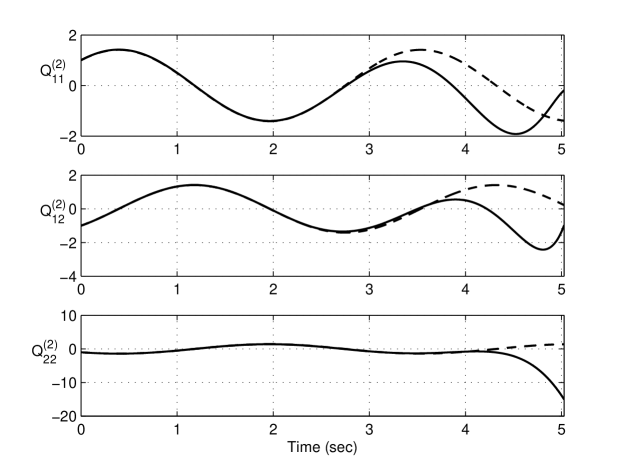
Figure 1: Determination of $Q^{(2)}_{t}$ for the Stuart-Landau oscillator with $a=2,b=1$. Each component of the tensors is plotted as a function of time. Numerical integration is done backward in time using the Euler method with $dt=10^{-3}$. Solid line: $Q^{(2)}_{t}$ determined from $A_{t,NT}$; dashed line: $Q^{(2)}_{t}$ found analytically. To clearly show convergence of the numerically obtained $Q^{(2)}_{t}$ to the analytical solution, $A_{t,NT}$ was not plotted and the period of the simulation was set at only $0.8T$.

We can now write the differential equations for $Q_{i}$ and $Q_{ij}$ (Equations 6 and 7; all summations are over $s=1,2$):

$$\dot{Q}_{i} =\sum_{s}Q_{s}F^{s}_{i}$$ (20)

$$\dot{Q}_{ij} =\sum_{s}(F_{i}^{s}Q_{sj}+F^{s}_{j}Q_{si})-\sum_{s}Q_{s}F^{s}_{ij}.$$ (21)

The first equation is the one used in the standard Malkin’s approach. Once it is solved by the already indicated procedure, its solution enters as the non-homogeneous term for the second equation.

The result of the numerical calculation is shown in Figure 1. The initial condition for $A_{t,NT}$ was chosen from a set of random numbers and numerical integration of Equations (21) was done backward in time (data not shown). Then, $Q^{(2)}_{t}$ was obtained using Equation (8) (solid line in Figure 1). Convergence of $Q^{(2)}_{t}$, obtained numerically, to the analytical solution (dashed line in Figure 1) is clearly observed.

2 Proof of the main theorem

The subsequent sections are dedicated to proving Theorem 1.1. It is convenient, for reasons we hope will become apparent along the way, to use a more geometric and coordinate-free language for manipulating tensors, even though all calculations are done in $\mathbb{R}^{n}$. This preparatory material on tensor calculus will take a few pages to develop, so it may be appropriate to provide an overview of the proof in simpler terms first.

The basic idea for proving part 1 of Theorem 1.1 is the following. An immediate consequence of the definition of the phase function is that $\Theta(\phi_{t}(\gamma(s)))=\omega t+\Theta(\gamma(s))$ for any differentiable curve $\gamma(s)$. Therefore, $\frac{d}{dt}\frac{d^{k}}{ds^{k}}\Theta(\phi_{t}(\gamma(s)))=0$ for $k\geq 1$. This gives an ODE that the $k$th derivative of the phase function must satisfy. Thus the proof of part 1 simply amounts to successive applications of elementary differentiation rules, although handling the multitude of terms that arise quickly becomes a challenge. In fact, this is precisely the kind of situation that often calls for the use of Faà di Bruno type formulas. We take here a different approach, which obtains the differential equation recursively and uses a coordinate-free language to facilitate the manipulation of terms.

The proof also involves a somewhat surprising cancellation of terms that renders the result more simple than might be expected at first. To better understand this point, we sketch the derivation of the differential equation in dimension one. Although the calculation is considerably more complicated in the general case, the key formal aspects of the derivation are already present for $n=1$. We use subscripts to indicate the number of derivatives, so $f_{k}(x)$ is the $k$th derivative of $f(x)$, whereas $f^{\prime}(x)$ is also used for the first derivative. Let $\gamma(s)=x_{0}+vs$, where $x_{0}$ and $v$ are fixed. Let $u_{t}(s)=\phi_{t}(\gamma(s))$, so $u_{t}^{\prime}(0)=\phi_{t}^{\prime}(x_{0})v$. Also set $Q^{(k)}_{t}(s)=\Theta_{k}(u_{t}(s))$. Recall that we wish to find a differential equation for $Q^{(k)}_{t}=Q^{(k)}_{t}(0)$. The differential equation associated to $F$ is $\dot{u}_{t}(s)=F(u_{t}(s))$. Then for $k=1$,

$$0=\frac{d}{dt}\frac{d}{ds}\Theta(\phi_{t}(\gamma(s)))=\left\{\dot{Q}^{(1)}_{t}(s)+Q^{(1)}_{t}(s)F_{1}(u_{t}(s))\right\}\phi_{t}^{\prime}(\gamma(s))v$$

for arbitrary $v$. An exchange of the order of derivatives in $t$ an $s$ was used in the second term of the right-hand side of the equation. Thus we conclude that $\dot{Q}^{(1)}_{t}(s)+F_{1}(u_{t}(s))Q^{(1)}_{t}(s)=0$, from which the claim for $k=1$ follows by taking $s=0$.

We now suppose that

$$\dot{Q}_{t}^{(j)}(s)+\sum_{l=1}^{j}\binom{j}{l}F_{l}(u_{t}(s))Q_{t}^{(j+1-l)}(s)=0$$

for $1\leq j\leq k$ and wish to show that this also holds for $j=k+1$. Taking one more derivative in $s$ and exchanging derivatives in $t$ and $s$ gives

$$\begin{split}0&=\frac{d}{ds}\left\{\frac{d}{dt}\Theta_{k}(u_{t}(s))+\sum_{l=1}^{k}\binom{k}{l}F_{l}(u_{t}(s))\Theta_{k+1-l}(u_{t}(s))\right\}\\ &=\left\{\dot{Q}_{t}^{(k+1)}(s)+Q_{t}^{(k+1)}(s)F_{1}(u_{t}(s))\right\}u^{\prime}_{t}(s)\\ &\qquad+\sum_{l=1}^{k}\binom{k}{l}\left\{F_{l+1}(u_{t}(s))Q_{t}^{(k+1-l)}(s)+F_{l}(u_{t}(s))Q_{t}^{(k+2-l)}(s)\right\}u^{\prime}_{t}(s).\end{split}$$

Thus the desired equation will hold for $j=k+1$ if we can show that

$$\begin{split}Q_{t}^{(k+1)}(s)F_{1}(u_{t}(s))&+\sum_{l=1}^{k}\binom{k}{l}\left\{F_{l+1}(u_{t}(s))Q_{t}^{(k+1-l)}(s)+F_{l}(u_{t}(s))Q_{t}^{(k+2-l)}(s)\right\}\\ &\qquad=\sum_{l=1}^{k+1}\binom{k+1}{l}F_{l}(u_{t}(s))Q^{(k+2-l)}_{t}(s).\end{split}$$

This indeed holds and is easily checked for $n=1$ by using the well-known relation

$$\binom{k}{l-1}+\binom{k}{l}=\binom{k+1}{l}.$$

The $n\geq 2$ case is considerably more involved but follows a similar line of proof.

Our use of tensor calculus becomes more essential in the proof of parts 2 and 3 of the main theorem, which rely on a study of the stability properties of the tensor equation given in part 1. Part 4 boils down to an enumeration of certain combinations of tensors that can be represented by formal linear combinations of rooted trees. This is discussed later under the heading “forest expansion.”

2.1 Higher order differentials of tensor fields

In this and the next two sections we develop some background material on differential calculus of tensor fields that will make our calculations of Taylor expansions of functions and vector fields more tractable. We suppose that the standard concepts (see, for example, [9]), such as tangent and cotangent bundles, Lie derivatives, covariant differentiation, etc, are known, but recall some of the definitions for the purpose of setting up notation.

Let $V$ be a finite dimensional vector space and $V^{*}$ its dual space. The space of tensors of type $(r,s)$ is

$$V^{(r,s)}=V\otimes\cdots\otimes V\otimes V^{*}\otimes\cdots\otimes V^{*},$$

in which there are $r$ copies of $V$ and $s$ copies of $V^{*}$. We think of an element of $V^{(r,s)}$ as an $s$-multilinear function taking values in the set of $(r,0)$-tensors. We find it useful to represent a tensor $T$ of type $(r,s)$ as a diagram consisting of a box with $s$ (contravariant) lower legs and $r$ (covariant) upper legs, and think of the lower legs as places where the vector arguments are plugged in. See for example, Figure 2.

A tensor field of type $(r,s)$ on $\mathbb{R}^{n}$ is a function that associates to each $x$ in $\mathbb{R}^{n}$ an element of $V_{x}^{(r,s)}$, where $V_{x}=T_{x}\mathbb{R}^{n}$ is the tangent space at $x$. (This tangent space is, of course, naturally identified with $\mathbb{R}^{n}$, but observing the distinction will help keep track of where derivatives are evaluated.)

All the tensor fields (functions, vector fields, etc.) that are considered below are smooth. The result of evaluating an $(r,s)$ tensor $T$ on $s$ vectors $X_{1},\dots,X_{s}$ is the $(r,0)$ tensor denoted $T(v_{1},\dots,v_{s})$.

Let $D$ be the standard covariant derivative in $\mathbb{R}^{n}$. If $X$ is a vector field and $v$ is a tangent vector at some point, then ${D}_{v}X$ is the standard derivative of $X$ along $v$. The derivative of an ordinary function $f$ along $v$ will be written as $vf={D}_{v}f$. We can then extend the definition ${D}_{v}$ to general tensors by imposing the condition that the product rule for differentiation holds for the tensor product $\otimes$ as well as for the pairing operation of $V$ and $V^{*}$. This implies that if $X_{1},\dots,X_{s}$ are vector fields and $v\in T_{x}\mathbb{R}^{n}$, then

$$({D}_{v}T)(X_{1},\dots,X_{s})={D}_{v}T(X_{1},\dots,X_{s})-\sum_{j=1}^{s}T(X_{1},\dots,{D}_{v}X_{j},\dots,X_{s}).$$ (22)

When $T$ has type $(0,s)$, $T(X_{1},\dots,X_{s})$ is an ordinary function, and we write $vT(X_{1},\dots,X_{s})$ instead of ${D}_{v}T(X_{1},\dots,X_{s})$. The result of the differentiation of $T$ is an $(r,s+1)$ tensor field ${D}T$.

Similarly, ${D}^{k}T$ is the $(r,s+k)$ tensor field obtained from $T$ by applying ${D}$ $k$-times. We call ${D}^{k}T$ the $k$-th order differential of $T$. Regarding $T^{(k)}={D}^{k}T$ as a $k$-multilinear map taking values in the space of $(r,s)$ tensors, then it can also be defined inductively: $T^{(1)}(v)={D}_{v}T$ and $T^{(k)}(v_{1},\dots,v_{k})=({D}_{v_{1}}T^{(k-1)})(v_{2},\dots,v_{k})$ for $k\geq 2$.

We are dealing with the standard covariant differentiation in $\mathbb{R}^{n}$, so ${D}$ is symmetric (i.e., its torsion tensor is 0) and flat (i.e., its curvature tensor is 0): given vector fields $X_{1},X_{2},X_{3}$, then ${D}_{X_{1}}X_{2}-{D}_{X_{2}}X_{1}=[X_{1},X_{2}]$ and ${D}_{X_{1}}{D}_{X_{2}}X_{3}-{D}_{X_{2}}{D}_{X_{1}}X_{3}={D}_{[X_{1},X_{2}]}X_{3}$, where $[X_{1},X_{2}]$ is the Lie bracket. We also say that an $(r,s)$-tensor field $S$ is symmetric if for each permutation $\sigma$ of the set $\{1,\dots,k\}$ and each $x$, $S_{x}^{(k)}(v_{\sigma(1)},\dots,v_{\sigma(k)})=S^{(k)}_{x}(v_{1},\dots,v_{k})$ for all vectors $v_{1},\dots,v_{k}\in T_{x}\mathbb{R}^{n}$. For simplicity, we are not indicating the $s$ vector arguments of $S$.

Proposition 2.1

Let $T$ be an $(r,s)$-tensor field in $\mathbb{R}^{n}$ and $T^{(k)}$ the $k$-th order differential of $T$. Then $T^{(k)}$ is symmetric.

Proof. We indicate the proof for $k=2$. The general case follows by induction using the same argument. Let $X_{1},X_{2}$ be vector fields that agree with $v_{1},v_{2}$ at $x$. If follows from the definitions that

$$T^{(2)}_{x}(v_{1},v_{2})={D}_{X_{1}}{D}_{X_{2}}T-{D}_{{D}_{X_{1}}X_{2}}T$$

where the right-hand side is evaluated at $x$. Therefore,

$$T^{(2)}_{x}(v_{1},v_{2})-T^{(2)}_{x}(v_{2},v_{1})=[{D}_{X_{1}},{D}_{X_{2}}]T-{D}_{[X_{1},X_{2}]}T=0,$$

where the last equality is due to the fact that ${D}$ is flat. $\square$

As an example, let $T$ be an ordinary function, denoted $f$. Let $X_{1},\dots,X_{n}$ be the coordinate vector fields in $\mathbb{R}^{n}$: $X_{j}=\frac{\partial}{\partial x_{j}}$. Then it is easy to check that

$$f^{(k)}(X_{j_{1}},\dots,X_{j_{k}})=X_{j_{1}}\dots X_{j_{k}}f,$$

which is the $k$-th order partial derivative of $f$ with respect to $x_{j_{1}},\dots,x_{j_{k}}$.

2.2 Symmetric composition of tensors

Let $S_{k}$ represent the group of permutations of the set $\{1,\dots,k\}$. Given a tensor $T$ of type $(r,k)$, we define its symmetrization $\widetilde{T}$ as the $(r,k)$-tensor derived from $T$ by symmetrizing its $k$ contravariant legs:

$$\widetilde{T}(v_{1},\dots,v_{k})=\frac{1}{k!}\sum_{\sigma\in S_{k}}T(v_{\sigma(1)},\dots,v_{\sigma{k}}).$$

If we need to symmetrize only a subset of the contravariant legs, this will be indicated in some explicit fashion. For example, if $T$ is an $(r,k+l)$-tensor, we separate by a semicolon the vector arguments that will not be symmetrized and place them last in order of insertion: $T(v_{1},\dots,v_{k};w_{1},\dots,w_{l}).$ Diagrammatically, the input legs taking the arguments $w_{1},\dots,w_{l}$ could be shown, for example, on either side of the tensor box, although we will simply omit them in our diagrams. A thick line crossing the other contravariant legs is added to indicate symmetrization.

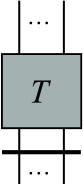
Figure 2: Diagram for the symmetrization of a $(r,k)$-tensor. The symmetrization of the contravariant legs is indicated by a thick bar.

It is convenient to introduce a binary operation on tensors, which we call symmetric composition. Let $Q$ be an $(r,s)$-tensor $Q$ and $H$ a $(l,k)$-tensor, where $l\leq s$. We define the symmetric $(r,s+k-l)$-tensor $Q\odot H$ as follows:

$$Q\odot H(v_{1},\dots,v_{s+k-l})=\frac{1}{(s+k-l)!}\sum_{\sigma\in S_{s+k-l}}Q(H(v_{\sigma(1)},\dots,v_{\sigma(k)}),v_{\sigma(k+1)},\dots,v_{\sigma(s+k-l)})$$

We have assumed here for simplicity that all the contravariant legs are involved in the symmetrization. The more general case is defined similarly.

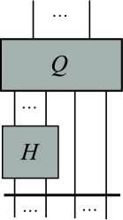
Figure 3: Symmetric composition $Q\odot H$ of $Q$ and $H$.

It is clear from the diagram that $Q\odot H$ would still make sense if $l>s$, in which case the result of the operation is a symmetric $(r+l-s,k)$-tensor. Below we mainly need the case where $l=1$. We also note that the input legs to which symmetrization is typically applied later in the paper are created from multiple applications of covariant differentiation to a tensor.

Proposition 2.2

The symmetric composition of $Q$ and $H$ satisfies the product rule:

$${D}_{v}(Q\odot H)=({D}_{v}Q)\odot H+Q\odot{D}_{v}H.$$

Proof. The proof is a tedious but straightforward application of Equation 22 and the easily proved fact that the $(k,k)$-tensor $P:v_{1}\otimes\dots\otimes v_{k}\rightarrow v_{\sigma(1)}\otimes\dots\otimes v_{\sigma(k)}$ satisfies ${D}P=0$, where $\sigma$ is any permutation. $\square$

When $Q$ and $H$ are themselves symmetric, $Q\odot H$ has the following useful description. Let $\mathcal{C}(k,l)$ represent the collection of all $l$-subsets of $\{1,\dots,k\}$ (i.e., subsets with $l$ elements). The cardinality of $\mathcal{C}(k,l)$ is the binomial coefficient $\binom{k}{l}=k!/(k-l)!l!$. Let $\pi:S_{k}\rightarrow\mathcal{C}(k,l)$ denote the map that associates to each permutation $\sigma$ the set $J=\{\sigma(1),\dots,\sigma(l)\}$, and write $S_{J}=\pi^{-1}(J)$. Then each $S_{J}$, $J\in\mathcal{C}(k,l)$, has cardinality $l!(k-l)!$ and $S_{k}$ is partitioned into the disjoint union of the $S_{J}$. The following notation will be used: let $v_{1},\dots,v_{k}$ be a subset of $T_{x}\mathbb{R}^{n}$, $H$ a symmetric $(m,l)$-tensor at $x$, and $J$ an $l$-subset of $\{1,\dots,k\}$. Then it makes sense to write $H(J):=H(v_{j_{1}},\dots,v_{j_{l}})$ for $J=\{j_{1},\dots,j_{l}\}.$ If $Q$ is a symmetric $(r,s)$-tensor, where $s\geq m$ and $s-m=k-l$, we similarly write $Q(H(J),J^{c})$, where $J^{c}$ indicates the complement of $J$. (More generally, $Q$ and $H$ may contain additional contravariant legs, with respect to which the tensors are not necessarily symmetric, that are not included in the operation of symmetric composition.)

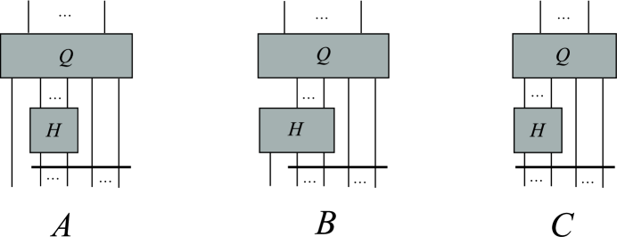
Figure 4: Tensors $A,B,C$ satisfying the identity $\binom{k-1}{l+1}A+\binom{k-1}{l}B=\binom{k}{l+1}C$ of Proposition 2.3.

If $v\in T_{x}\mathbb{R}^{n}$ and $H$ is an $(l,k)$-tensor, let $i_{v}H$ denote the $(l,k-1)$-tensor such that $(i_{v}H)(v_{2},\dots,v_{k})=H(v,v_{2},\dots,v_{k})$.

Proposition 2.3

Let $H$ be an $(u,l+1)$-tensor, $Q$ an $(m,k-l-1+u)$-tensor, both symmetric in their lower legs, and $v\in T_{x}\mathbb{R}^{n}$. Then

$$\binom{k}{l+1}i_{v}(Q\odot H)=\binom{k-1}{l+1}i_{v}Q\odot H+\binom{k-1}{l}Q\odot i_{v}H.$$

Proof. Let $v_{1}=v$, $v_{2},\dots,v_{k}$ be elements of $T_{x}\mathbb{R}^{n}$. The key point to observe is that the sum of $Q(H(J),J^{c})$ over all $J\in\mathcal{C}(k,l+1)$ is equal to the sum over all $J\in\mathcal{C}(k,l+1)$ that contain $1$ plus the sum over all $J$ that do not. $\square$

2.3 Identities for the Lie derivative

The infinitesimal action of the flow $\phi_{t}$ on tensors is given by the Lie derivative with respect to the vector field $F$. We register here for later use some useful formulas involving the Lie and covariant derivatives. We recall that the Lie derivative of tensor fields is defined just as we did for the covariant derivative, except that, on a vector field $X$, it is given by the Lie bracket $\mathcal{L}_{F}X=[F,X]$, and on functions $\mathcal{L}_{F}f=Ff$. Another way to describe $\mathcal{L}_{F}T$ is as the time derivative of the tensor defined by “convecting” $T$ along the flow of $F$.

Let now $F$ be a smooth vector field (thus $F$ is a $(1,0)$-tensor) and set $F^{(k)}={D}^{k}F$. Thus $F^{(k)}$ is a $(1,k)$-tensor. For the moment, we only make use of $F^{(1)}$.

The covariant and Lie derivatives of tensors with respect to a vector field $F$ are related via an “algebraic derivative” with respect to $F^{(1)}$. The latter operation is defined as follows. Let $B$ be a field of linear maps and define $\mathcal{A}_{B}$ by the properties: (1) $\mathcal{A}_{B}f=0$ on functions; (2) $\mathcal{A}_{B}v=Bv$ on vectors; (3) $\mathcal{A}_{B}\alpha=-\alpha\circ B$ on covectors; (4) $\mathcal{A}_{B}$ satisfies the product rule with respect to tensor product. It can be checked that these properties uniquely determine a linear map on tensors. In particular, if $Q$ is a $(0,k)$-tensor,

$$(\mathcal{A}_{B}Q)(v_{1},\dots,v_{k})=-\sum_{j=1}^{k}Q(v_{1},\dots,Bv_{j},\dots,v_{k}).$$

From the properties stated in Proposition 2.4 below we obtain that if $Q$ is a $(0,k)$-tensor field, then for any point $x$ and tangent vectors $v_{1},\dots,v_{k}$ at $x$,

$$(\mathcal{L}_{F}Q)_{x}(v_{1},\dots,v_{k})=({D}_{F}Q)_{x}(v_{1},\dots,v_{k})+\sum_{j=1}^{k}Q_{x}(v_{1},\dots,F^{(1)}(v_{j}),\dots,v_{k}),$$

and if moreover $Q$ is symmetric, then $\mathcal{L}_{F}Q={D}_{F}Q+kQ\odot F^{(1)}.$ The next proposition summarizes some relations among the various derivative operations. Here $[\cdot,\cdot]$ is the standard commutator of operators. Also note that, if we regard $F$ as generating the time evolution of a system, then with a slight abuse of notation, ${D}_{F}Q=\dot{Q}$, where the dot over $Q$ means time derivative. Below, $F^{(l+1)}(X_{1},\dots,X_{l},\cdot)$ is the field of linear maps defined by inserting a vector into the last slot.

Proposition 2.4

Let $F$, $X$, $X_{1},\dots,X_{l}$ be vector fields and $Q$ an $(r,k)$-tensor field. Then

1. ${D}_{F}Q-\mathcal{L}_{F}Q=\mathcal{A}_{F^{(1)}}Q$

2. $[{D}_{X},\mathcal{A}_{F^{(1)}}]Q=\mathcal{A}_{F^{(2)}(X,\cdot)}Q$

3. $[{D}_{X_{1}},\mathcal{A}_{F^{(l)}(X_{2},\dots,X_{l},\cdot)}]=\mathcal{A}_{F^{(l+1)}(X_{1},\dots,X_{l},\cdot)+\sum_{j=2}^{l-1}F^{(l)}(X_{2},\dots,{D}_{X_{1}}X_{j},\dots,X_{l},\cdot)}$

4. $[\mathcal{L}_{F},{D}_{X}]Q={D}_{[F,X]}Q+\mathcal{A}_{F^{(2)}(X,\cdot)}Q$

5. $(\mathcal{L}_{F}Q^{(1)})(X;\cdot)={D}_{X}\mathcal{L}_{F}Q+\mathcal{A}_{F^{(2)}(X,\cdot)}Q.$

Proof. It is easily checked that ${D}_{F}-\mathcal{L}_{F}$ has the properties defining $\mathcal{A}_{F^{(1)}}$, so 1 is a consequence of uniqueness of $\mathcal{A}_{F^{(1)}}$. A similar verification also proves 2. Property 3 is shown by induction and the same argument used for 1 and 2 based on uniqueness of the algebraic derivative. Properties 4 and 5 can be proved using 1 and 2 by a tedious but straightforward algebraic manipulation. When deriving these properties, it should be born in mind that ${D}$ is torsion-free and flat. $\square$

Property 5 of the above proposition gives a way of finding $\mathcal{L}_{F}Q^{(k)}$ recursively if $\mathcal{L}_{F}Q$ is known. We illustrate this with a formula for $\mathcal{L}_{F}Q$ when $Q=f^{(k)}$ and $f$ is a function. This is the case we need to consider in extending Malkin’s method. The key point to notice is that the formula expresses $\mathcal{L}_{F}f^{(k)}$ in terms of the lower order tensors $f^{(l)}$, $l=1,\dots,k-1$.

Proposition 2.5

Let $F$ be a smooth vector field and $f$ a smooth function. Suppose that $Ff=g$, for some smooth function $g$. Then $\mathcal{L}_{F}f^{(1)}=g^{(1)}$ and, for $k\geq 2$,

$$\mathcal{L}_{F}f^{(k)}=g^{(k)}-\sum_{l=2}^{k}\binom{k}{l}f^{(k+1-l)}\odot F^{(l)}.$$

Proof. The proof is by induction. Using Property 5 of Proposition 2.4 one immediately gets $\mathcal{L}_{F}f^{(1)}=g^{(1)}$ and

$$\left(\mathcal{L}_{F}f^{(2)}\right)(v_{1},v_{2}) =\left({D}_{v_{1}}\mathcal{L}_{F}f^{(1)}\right)(v_{2})+\left(\mathcal{A}_{F^{(2)}(v_{1},\cdot)}f^{(1)}\right)(v_{2})$$

$$=\left({D}_{v_{1}}g^{(1)}\right)(v_{2})-f^{(1)}\left(F^{(2)}(v_{1},v_{2})\right)$$

$$=\left(g^{(2)}-f^{(1)}\odot F^{(2)}\right)(v_{1},v_{2}).$$

So we suppose that the equation holds for $k\geq 2$ and wish to obtain it for $k+1$. First note that

$$\begin{split}\left({D}_{v_{1}}\mathcal{L}_{F}f^{(k)}\right)(v_{2},\dots,v_{k+1})&={D}_{v_{1}}\left(g^{(k)}-\sum_{l=2}^{k}\binom{k}{l}f^{(k+1-l)}\odot F^{(l)}\right)(v_{2},\dots,v_{k+1})\\ &=g^{(k+1)}(v_{1},\dots,v_{k+1})\\ &\qquad-\sum_{l=2}^{k}\binom{k}{l}\left({D}_{v_{1}}f^{(k+1-l)}\odot F^{(l)}\right)(v_{2},\dots,v_{k+1})\\ &\qquad\qquad-\sum_{l=2}^{k}\binom{k}{l}\left(f^{(k+1-l)}\odot{D}_{v_{1}}F^{(l)}\right)(v_{2},\dots,v_{k+1})\\ &=g^{(k+1)}(v_{1},\dots,v_{k+1})\\ &\qquad-\sum_{l=1}^{k-1}\binom{k}{l+1}\left({D}_{v_{1}}f^{(k-l)}\odot F^{(l+1)}\right)(v_{2},\dots,v_{k+1})\\ &\qquad\qquad-\sum_{l=1}^{k-1}\binom{k}{l}\left(f^{(k+1-l)}\odot{D}_{v_{1}}F^{(l)}\right)(v_{2},\dots,v_{k+1})\\ &\qquad\qquad\qquad-\left(f^{(1)}\odot F^{(k+1)}\right)(v_{1},\dots,v_{k+1})\\ &\qquad\qquad\qquad\qquad+k\left(f^{(k)}\odot{D}_{v_{1}}F^{(1)}\right)(v_{2},\dots,v_{k+1}).\end{split}$$

Using the tensor identity of Proposition 2.3, the above simplifies to

$$\begin{split}\left({D}_{v_{1}}\mathcal{L}_{F}f^{(k)}\right)(v_{2},\dots,v_{k+1})&=g^{(k+1)}(v_{1},\dots,v_{k+1})\\ &\qquad-\sum_{l=2}^{k+1}\binom{k+1}{l}\left(f^{(k+2-l)}\odot F^{(l)}\right)(v_{1},\dots,v_{k+1})\\ &\qquad\qquad+k\left(f^{(k)}\odot{D}_{v_{1}}F^{(1)}\right)(v_{2},\dots,v_{k+1}).\end{split}$$

By Property 5 of Proposition 2.4,

$$\begin{split}\mathcal{L}_{F}f^{(k+1)}(v_{1},\dots,v_{k+1})&=\left({D}_{v_{1}}\mathcal{L}_{F}f^{(k)}\right)(v_{2},\dots,v_{k+1})+\left(\mathcal{A}_{F^{(2)}(v_{1},\cdot)}f^{(k)}\right)(v_{2},\dots,v_{k+1})\\ &=\left({D}_{v_{1}}\mathcal{L}_{F}f^{(k)}\right)(v_{2},\dots,v_{k+1})\\ &\qquad-\sum_{j=2}^{k+1}f^{(k)}(v_{2},\dots,F^{(2)}(v_{1},v_{j}),\dots,v_{k+1})\\ &=g^{(k+1)}(v_{1},\dots,v_{k+1})\\ &\qquad-\sum_{l=2}^{k+1}\binom{k+1}{l}\left(f^{(k+2-l)}\odot F^{(l)}\right)(v_{1},\dots,v_{k+1})\\ &\qquad\qquad+k\left(f^{(k)}\odot{D}_{v_{1}}F^{(1)}\right)(v_{2},\dots,v_{k+1})\\ &\qquad\qquad\qquad-\sum_{j=2}^{k+1}f^{(k)}(v_{2},\dots,F^{(2)}(v_{1},v_{j}),\dots,v_{k+1})\\ &=g^{(k+1)}(v_{1},\dots,v_{k+1})\\ &\qquad-\sum_{l=2}^{k+1}\binom{k+1}{l}\left(f^{(k+2-l)}\odot F^{(l)}\right)(v_{1},\dots,v_{k+1}),\end{split}$$

which is the claimed formula for $k+1$. $\square$

The case of main interest is $f=\Theta$, for which $F\Theta=1/T$ is constant. Thus $g^{(k)}=0$ for $k\geq 1$ and we obtain

$$\mathcal{L}_{F}\Theta^{k}=-\sum_{l=2}^{k}\binom{k}{l}\Theta^{(k+1-l)}\odot F^{(l)}.$$ (23)

2.4 Proof of Theorem 1.1

We turn now to the proof of Theorem 1.1. Part (1) of the theorem, which gives the differential equation satisfied by $\Theta^{(k)}$ is restated in the next proposition. Recall the notation: $Q^{(k)}_{t}=\Theta^{(k)}_{\phi_{t}(x)},$ where $\phi_{t}$ is the flow of $F$ and $x$ is arbitrary. Indicating the time derivative of $Q^{(k)}$ by $\dot{Q}^{(k)}$, we have $\dot{Q}^{(k)}_{t}=({D}_{F}\Theta^{(k)})_{\phi_{t}(x)}.$

Proposition 2.6

We assume the notation of Section 1.3. Let $Q^{(k)}$ be as just defined. Then

$$\dot{Q}_{t}^{(k)}+kQ_{t}^{(k)}\odot F^{(1)}=-\sum_{l=1}^{k-1}\binom{k}{l+1}Q_{t}^{(k-l)}\odot F^{(l+1)}.$$

Proof. According to Proposition 2.4, ${D}_{F}\Theta^{(k)}-\mathcal{A}_{F^{(1)}}\Theta^{(k)}=\mathcal{L}_{F}\Theta^{(k)}$. On the other hand, $\mathcal{A}_{F^{(1)}}\Theta^{(k)}=-k\Theta^{(k)}\odot F^{(1)}$, and since the directional derivative $F\Theta$ is constant, $\mathcal{L}_{F}\Theta^{(k)}$ is given by Equation 23. We get the claimed formula by finally rewriting the resulting equation in terms of $Q^{(k)}_{t}$. $\square$

In what follows, let $W_{t}$ be the tangent space to the isochron at $\phi_{t}(x)$, $x\in\mathcal{C}$. Vectors in $W_{t}$, by assumption, contract exponentially under the flow; i.e., $|d\phi_{s}v|<C\lambda^{s}|v|$ for all $v\in W_{t}$ and positive constants $C$ and $\lambda<1$, where $s\geq 0$. If $v$ is parallel to $F(\phi_{t}(x))$ then $|d\phi_{s}v|$ is bounded above as well as away from $0$. We similarly need to know the decay properties of tensors of type $(0,k)$ under the flow. The natural push-forward action of $\phi_{s}$ on a tensor-valued function, $\tau_{t}$, of type $(0,k)$ along $\mathcal{C}$ is defined by

$$(\phi_{s}\cdot\tau_{t})(u_{1},\dots,u_{k})=\tau_{t}((d\phi_{s})_{y}^{-1}u_{1},\dots,(d\phi_{s})_{y}^{-1}u_{k}),$$

where $u_{1},\dots,u_{k}$ are vectors at $y$. This applies, in particular, to a tensor field $\tau$ defined in a neighborhood of $\mathcal{C}$, in which case $\tau_{t}=\tau_{\phi_{t}(x)}$ is a $T$-periodic tensor-valued function of $t$. The function is flow-invariant if $\phi_{s}\cdot\tau_{t}=\tau_{t+s}$.

Let $\mathbb{R}\tau$ represent the one-dimensional space over $\mathbb{R}$ spanned by a tensor $\tau$. Since the family of isochrons and the vector field $F$ are invariant under the flow, the tangent space to $\mathbb{R}^{n}$ decomposes invariantly as a direct sum

$$T_{\phi_{t}(x)}\mathbb{R}^{n}=\mathbb{R}F_{t}\oplus W_{t},$$

where $F_{t}=F(\phi_{t}(x))$. Let $W_{t}^{*}$ be the subspace of $T^{*}_{\phi_{t}(x)}\mathbb{R}^{n}$ consisting of covectors that vanish on $F_{t}$. It is not difficult to check that

$$T^{*}_{\phi_{t}(x)}\mathbb{R}^{n}=\mathbb{R}Q^{(1)}_{t}\oplus W_{t}^{*}$$

is also a flow-invariant decomposition. By general tensor algebra, one also obtains a flow-invariant decomposition of the space of $(0,k)$-tensors as a direct sum of subspaces of the form

$$V_{k_{1},k_{2},t}=\mathbb{R}Q_{t}^{(1)}\otimes\cdots\otimes\mathbb{R}Q_{t}^{(1)}\otimes W_{t}^{*}\otimes\cdots\otimes W_{t}^{*},$$

in which there are $k_{1}$ copies of $\mathbb{R}Q_{t}^{(1)}$ and $k_{2}$ copies of $W_{t}^{*}$, where $k_{1}+k_{2}=k$ and $0\leq k_{1}\leq k$.

The Euclidean norm on vectors, $|v|$, extends in natural ways to norms on tensors of any kind. We use the same notation, $|\tau|$, for the norm of a tensor $\tau$ of general type. We refer the reader to texts on multilinear algebra or differential geometry for how this can be defined, although it is not necessary for what we do below to have any explicit description in mind, and the form of the theorem does not depend on a particular choice of norm. The main property we use below is that if $A$ is a $(0,k)$-tensor and $u_{1},\dots,u_{k}$ are vectors then $|A(u_{1},\dots,u_{k})|\leq|A|\prod_{j=1}^{k}|u_{j}|$.

Lemma 2.1

Let $A$ be a tensor in $V_{k_{1},k_{2},t}$. Then there exists a constant $C_{A}$ such that $|\phi_{s}\cdot A|\leq C_{A}\lambda^{k_{2}|s|}$ for all $s<0$.

Proof. A tensor in $V_{k_{1},k_{2},t}$ has the form $Q_{t}^{(1)}\otimes\cdots\otimes Q_{t}^{(1)}\otimes\widetilde{A}$ where $\widetilde{A}$ belongs to the $k_{2}$-fold tensor power of $W_{t}^{*}$. Thus $|\phi_{s}\cdot A|\leq K|\phi_{s}\cdot\widetilde{A}|$, where $K$ is the $k_{1}$th power of the supremum of $|Q_{s}^{(1)}|$ over the period $0\leq s\leq T$. Since $\widetilde{A}$ vanishes whenever any one of its arguments is parallel to $F_{t}$, the norm of $\phi_{s}\cdot\widetilde{A}$ can be bounded above by the supremum of $|\widetilde{A}((d\phi_{s})^{-1}u_{1},\dots,(d\phi_{s})^{-1}u_{1})|$ over all $u_{j}\in W_{t+s}$ of norm at most $1$. Now,

$$\left|\widetilde{A}((d\phi_{s})^{-1}u_{1},\dots,(d\phi_{s})^{-1}u_{1})\right|\leq\left|\widetilde{A}\right|\prod_{j=1}^{k_{2}}\left|(d\phi_{s})^{-1}u_{j}\right|\leq C^{k_{2}}\lambda^{k_{2}|s|}$$

which proves the assertion of the lemma. $\square$

Proposition 2.7

Let $x\in\mathcal{C}$ and $A_{t}^{(k)}$ a $(0,k)$-tensor at $\phi_{t}(x)$ depending differentiably on $t$. Suppose that $A^{(k)}_{t}$ is a solution of the homogeneous equation

$$\dot{A}_{t}^{(k)}+kA^{(k)}_{t}\odot F^{(1)}=0.$$

Then for some positive constant $K$ and for $\lambda<1$ as above, there exists $c$ such that

$$\left|A_{t}^{(k)}-c\ \!Q_{t}^{(1)}\otimes\cdots\otimes Q_{t}^{(1)}\right|<K\lambda^{|t|}$$

for all $t<0$, where the tensor product on the left-hand side contains $k$ terms. In particular, if $A_{t}^{(k)}$ is $T$-periodic, then $A_{t}^{(k)}=c\ \!Q_{t}^{(1)}\otimes\cdots\otimes Q_{t}^{(1)}$.

Proof. Since $F_{x}=\frac{d}{dt}$ along the limit cycle (by the usual identification of a vector field as a derivation), $\dot{A}_{t}$ equals ${D}_{F}A$, where the latter has to be interpreted in terms of an arbitrary extension of $A$ on a neighborhood of the limit cycle. Now, according to part (1) of Proposition 2.4,

$$\mathcal{L}_{F}A_{t}^{(k)}=\dot{A}_{t}^{(k)}-\mathcal{A}_{F^{(1)}}A_{t}^{(k)}=\dot{A}^{(k)}+kA^{(k)}\odot F^{(1)}=0$$

on $\mathcal{C}$. Therefore, the proposition amounts to the assertion that (1) the space of periodic, flow-invariant tensor-valued functions of type $(0,k)$ on $\mathcal{C}$ is one-dimensional, spanned by the $k$th tensor power of $Q_{t}^{(1)}$, and (2) if $A_{t}^{(k)}$ is flow-invariant but not necessarily periodic, the stated inequality holds, i.e., the components of a solution transverse to the one-dimensional space of periodic solutions must contract exponentially to $0$.

Thus suppose first that $A_{t}^{(k)}$ is flow-invariant and $T$-periodic. Let $A_{t}^{(k_{1},k_{2})}$ be the component of $A_{t}^{(k)}$ in $V_{k_{1},k_{2},t}$. In particular, $A^{(k,0)}_{t}=c_{t}Q_{t}^{(1)}\otimes\cdots\otimes Q_{t}^{(1)}$. Since the subspaces $V_{k_{1},k_{2},t}$ are flow-invariant and periodic, each component $A_{t}^{(k_{1},k_{2})}$ is also flow-invariant and periodic. In particular, $c_{t}$ is constant (independent of $t$) and $A_{t}^{(k_{1},k_{2})}=0$ whenever $k_{2}\neq 0$, by Lemma 2.1. This shows claim (1). To verify claim (2) we suppose that $A_{t}^{(k)}$ is flow-invariant but not necessarily periodic. Thus $A_{t+s}^{(k)}=\phi_{s}\cdot A_{t}^{(k)}$. Now each component in the decomposition

$$A_{t}^{(k)}=c_{t}Q_{t}^{(1)}\otimes\cdots\otimes Q_{t}^{(1)}+\sum_{k_{2}\neq 0}A_{t}^{(k_{1},k_{2})}$$

is flow-invariant, so $c_{t+s}=c_{t}$ for all $s$ and

$$\left|A_{t+s}^{(k)}-c_{t}Q_{t+s}^{(1)}\otimes\cdots\otimes Q_{t+s}^{(1)}\right| \leq\sum_{k_{2}\neq 0}\left|A_{t+s}^{(k_{1},k_{2})}\right|$$

$$=\sum_{k_{2}\neq 0}\left|\phi_{s}\cdot A_{t}^{(k_{1},k_{2})}\right|$$

$$\leq K\lambda^{|s|}$$

for some constant $K$, where we have used again Lemma 2.1. This concludes the proof of the proposition. $\square$

We can now prove parts (2) and (3) of Theorem 1.1. For $k=1$, the equation reduces to

$$\dot{Q}_{t}^{(1)}+Q_{t}^{(1)}\circ F^{(1)}=0.$$

This equation can be solved numerically by the standard (first order) approach, which essentially amounts to Proposition 2.7 in the special case $k=1$: Fix $x\in\mathcal{C}$ and let $A$ be a choice of initial value, arbitrary except for the condition $A(F_{x})=1/T$. One then integrates the first order equation for $t<0$ for large enough values of $|t|$ until the solution stabilizes to a periodic matrix-valued function over the limit cycle. That function is the sought after solution for $Q_{t}^{(1)}$. For larger values of $k$, we regard the differential equation in Proposition 2.6 as non-homogeneous:

$$\dot{Q}_{t}^{(k)}+kQ^{(k)}_{t}\odot F^{(1)}=B^{(k)}_{t},$$

where the right-hand side is assumed to have already been obtained in the previous steps.

We proceed by induction. Suppose that we have found $Q^{(1)}_{t},\dots,Q^{(k-1)}_{t}$ and wish to obtain $Q^{(k)}_{t}$. Set

$$B_{t}^{(k)}=-\sum_{l=1}^{k-1}\binom{k}{l+1}Q_{t}^{(k-l)}\odot F^{(l+1)}$$ (24)

and integrate the equation

$$\dot{A}_{t}^{(k)}+kA^{(k)}_{t}\odot F^{(1)}=B^{(k)}_{t}$$

for $t\leq 0$, starting with an arbitrary initial condition, until ${A}_{t}^{(k)}$ stabilizes to a periodic function of $t$. Stabilization must occur at the exponential rate given by Proposition 2.7, since the difference ${A}_{t}^{(k)}-Q_{t}^{(k)}$ is a solution of the homogeneous equation of Proposition 2.7. This periodic solution is still denoted by $A_{t}^{(k)}$ (in particular, $A^{(k)}_{0}$ is the value at $x$ after stabilization). The true solution we seek, $Q^{(k)}_{t}$, differs from $A_{t}^{(k)}$ by a periodic homogeneous solution so there exists a constant $c$ such that

$$Q^{(k)}_{t}=A^{(k)}_{t}+c\ \!Q_{t}^{(1)}\otimes\cdots\otimes Q_{t}^{(1)}.$$

Since $Q^{(1)}_{t}(F)=1/T$, the constant $c$ has the form

$$c=T^{k}[Q_{0}^{(k)}(F_{x},\dots,F_{x})-A^{(k)}_{0}(F_{x},\dots,F_{x})].$$

It remains to argue that $Q_{0}^{(k)}(F_{x},\dots,F_{x})$ can be expressed in terms of the lower order $Q^{(l)}_{0}$, $F$, and its derivatives at $x$. Recall that $Q_{t}^{(k)}=\Theta^{(k)}_{\phi_{t}(x)}$. The following general fact holds for $\Theta^{(k)}_{y}$ (for $y$ not necessarily on the limit cycle). We set $F^{(0)}=F$.

Proposition 2.8

There exists for each $k$ an algebraic function that gives $\Theta^{(k)}_{y}(F_{y},\dots,F_{y})$ in terms of the $\Theta^{(l)}_{y}$, for $l=1,\dots,k-1$, and the $F^{(j)}_{y}$, for $j=0,\dots,k-1$, and $y$ in a neighborhood of $\mathcal{C}$.

The precise meaning of this proposition, and an algorithm for obtaining the indicated algebraic function, are explained and illustrated in the next section.

2.5 Forest expansion of $F^{k}\Theta$

We wish to expand $\Theta^{(k)}(F,\dots,F)$, at any given point, in terms of the $\Theta^{(j)}$ and $F^{(j)}$ for $j<k$, and thus find the algebraic function indicated in Proposition 2.8. This can naturally be done by successive applications of the chain rule, applied to the expression $F^{k}\Theta=0$, $k\geq 2$. (Recall that $F\Theta=\Theta^{(1)}(F)=1/T$.) What is needed is a method to conveniently deal with the combinatorial task of enumerating the terms of this expansion. This can be done by enumerating rooted trees with $k$ edges. We describe here this forest expansion method and illustrate it with a few examples.

Finding the general form of the algebraic function claimed in Proposition 2.5 for an arbitrary $k$ is a complicated combinatorial problem, and amounts to a type of Faà di Bruno formula, which we do not attempt to describe here. We are content with giving the forest expansin algorithm and applying it to small values of $k$.

Figure 5 explains how to represent nested evaluations of tensors by rooted trees. The number of edges of the rooted tree diagram is the total order of differentiation, so all diagrams associated to $F^{k}\Theta$ will contain $k$ edges. The degree of the root vertex is the order of differentiation of $\Theta$ (this is $3$ in the example of Figure 5), and all the other vertices represent a $F^{(j)}$, where $j+1$ is the vertex degree. Thus to each leaf (i.e., a vertex with no descendants) is attached an $F$, and to each non-root vertex is recursively attached a vector as follows: Starting from the leaves (associated to copies of $F$) one moves down one step to the parent vertices (associated to copies of $F^{(j)}$, if $j+1$ is the degree of a parent vertex) and compute $F^{(j)}(F,\dots,F)$. This vector is now attached to each of those second-to-last generation vertices. These new vectors in turn are evaluated into the tensors attached to their parent vertices. We continue this process until the vectors attached to the first generation vertices (the ones connected to the root by an edge) are evaluated into $\Theta^{(l)}$, where $l$ is the degree of the root vertex.

Figure 5: A rooted tree diagram representing $\Theta^{(3)}(F^{(2)}(F^{(3)}(F,F,F),F^{(1)}(F)),F,F)$, which is one term in the expression of $F^{9}\Theta$. The tree itself will be represented by $\tau_{3}(\tau_{2}(\tau_{3},\tau_{1}),\tau_{0},\tau_{0})$.

The expression $\Theta^{(k)}(F,\dots,F)$ itself corresponds to a tree having a root of order $k$ and $k$ leaves attached to it. We denote this tree by $\tau_{k}$, $k\geq 0$, where $\tau_{0}$ consists of a vertex with $0$ edges, i.e., a leaf. Other trees are obtained by nesting trees of type $\tau_{j}$. Thus each $\tau_{j}$ can take $j$ arguments, each of which is a tree of the same kind (for possibly different $j$). For example, $\tau_{l}(\tau_{j_{1}},\dots,\tau_{j_{l}})$ represents a tree that consists of a root vertex of degree $l$ and at the non-root vertex of each of the $l$ edges is appended the tree $\tau_{j_{s}}$ so that the root vertex of the latter is identified with the non-root vertex of the former.

It is clear that $F^{k}\Theta$ can in general be represented by a forest of rooted trees with $k$ edges, each tree being assigned some multiplicity. We will see shortly how the multiplicities are determined by counting the ways a tree is derived from other trees with $k-1$ edges. Figure 2.5 shows the forest diagram representation of $F^{2}\Theta$, $F^{3}\Theta$ and $F^{4}\Theta$.

We give a few examples of the forest expansion before showing the general method. By the basic rules of covariant differentiation of tensors, we obtain $FF\Theta=F\Theta^{(1)}(F)=\Theta^{(2)}(F,F)+\Theta^{(1)}(F^{(1)}(F)).$ Therefore,

$$\Theta^{(2)}(F,F)=-\Theta^{(1)}(F^{(1)}(F)).$$

For $k=3$, we have:

$$FFF\Theta =F[\Theta^{(2)}(F,F)+\Theta^{(1)}(F^{(1)}(F))]$$

$$=\Theta^{(3)}(F,F,F)+3\Theta^{(2)}(F^{(1)}(F),F)+\Theta^{(1)}(F^{(2)}(F,F))+\Theta^{(1)}(F^{(1)}(F^{(1)}(F))),$$

so that

$$-\Theta^{(3)}(F,F,F)=3\Theta^{(2)}(F^{(1)}(F),F)+\Theta^{(1)}(F^{(2)}(F,F))+\Theta^{(1)}(F^{(1)}(F^{(1)}(F))).$$

The expansion of $-\Theta^{(4)}(F,F,F,F)$ is shown diagrammatically in Figure 6.

Figure 6: The forest representation of $-\Theta^{(k)}(F,\cdots,F)$ for $k=2,3,4$.

It should now be apparent that the algebraic expression giving $-\Theta^{(k)}(F,\dots,F)$ as a function of the lower order terms $\Theta^{(j)}$ and the $F^{(l)}$, as claimed in Proposition 2.5, is precisely the forest expansion of $-\Theta^{(k)}(F,\dots,F)$. It is also clear that all rooted trees with $k$ edges (except $\tau_{k}$), up to isomorphism, appear as a term in the forest expansion of $\tau_{k}$, for a given $k$. What is needed then is a more formal description of how to determine the integer coefficients of the expansion. (Notice our slight abuse of language in referring to the forest expansion of $F^{k}\Theta$ or of $-\Theta^{(k)}(F,\dots,F)$ as the same thing. Of course, the expansion of the former contains one extra term, which is (minus) the latter.)

Let $\mathcal{T}(k)$ denote the set of (isomorphism classes of) rooted trees with $k$ edges, $k\geq 0$, and denote by $m:\mathcal{T}(k)\rightarrow\mathbb{N}\cup\{0\}$ the multiplicity function, which assigns to each tree its coefficient in the forest expansion of $F^{k}\Theta$. As already defined, each tree gives rise to a number: to the root vertex we associate $\Theta^{(l)}$, where $l$ is the vertex degree; to each of the other vertices we associate $F^{(j)}$, where $j$ is the degree of the respective vertex and $F^{(0)}=F$; the tensors are then evaluated as prescribed by the tree so that each vector attached to a vertex is an argument of the tensor attached to the parent vertex. The result of this nested evaluation of tensors for a given $T\in\mathcal{T}(k)$ will be written $T(\Theta,F)$. Therefore,

$$F^{k}\Theta=\sum_{T\in\mathcal{T}(k)}m(T)T_{p}(\Theta,F).$$

Thus, the forest expansion of $F^{k}\Theta$ requires an enumeration of all rooted trees with $k$ edges, and the determination of the multiplicities $m(T)$.

A few more definitions are needed before identifying $m$. A tree $T^{\prime}\in\mathcal{T}(k)$ is said to grow into $T\in\mathcal{T}(k+1)$ if $T$ can be obtained from $T^{\prime}$ by adding (grafting) one terminal edge to any vertex of $T^{\prime}$. Conversely, $T$ is pruned down to $T^{\prime}$ if $T^{\prime}$ results by eliminating a terminal edge from $T$. Let $\mathcal{C}_{k}$ be the $\mathbb{N}$-module consisting of linear combinations over $\mathbb{N}$ of elements of $\mathcal{T}(k)$. The dual of $T\in\mathcal{T}(k)$ will be written as $T^{*}$, so that $T^{*}(\sum_{S\in\mathcal{T}(k)}n_{S}S)=n_{T}.$

The pruning map $\mathcal{P}:\mathcal{T}(k+1)\rightarrow\mathcal{C}_{k}$ is defined as follows: For each $T\in\mathcal{T}(k+1)$ we set $\mathcal{P}(T)$ to be the sum of all distinct trees in $\mathcal{T}(k)$ which can grow into $T$. The grafting map $\mathcal{G}:\mathcal{C}_{k}\rightarrow\mathcal{C}_{k+1}$ is defined on a tree $T$ by summing all trees that can be pruned down to $T$, now counting repetitions (i.e., each tree is counted as many times as it appears in the process of grafting an edge at the different vertices), then multiplying the result by $m(T)$. Now extend $\mathcal{G}$ to $\mathcal{C}_{k}$ by linearity. It can be shown that the multiplicity function has the form:

$$m(T)=T^{*}(\mathcal{G}(\mathcal{P}(T))).$$

This is based simply on translating into diagrams the rule: If $A=F^{(s)}(A_{1},\dots,A_{s})$, then ${D}_{F}A=F^{(s+1)}(F,A_{1},\dots,A_{s})+\sum_{j=1}^{s}F^{(s)}(A_{1},\dots,{D}_{F}A_{j},\dots,A_{s}).$ The first term on the right corresponds to adding an edge to the root of the tree associated to $A$; the other terms on the right correspond to moving up one step along one of the root edges of $A$ and repeating the operation.

We illustrate the procedure for finding multiplicities with the example of $\tau_{k}(\tau_{1},\tau_{0},\dots,\tau_{0})$ shown in Figure 7. We use the shorter notation $\tau_{k,1}$ for this tree.

Figure 7: The rooted tree $\tau_{k,1}=\tau_{k}(\tau_{1},\tau_{0},\dots,\tau_{0})$. The pruning of the single edge at distance $2$ from the root gives $\tau_{k}$, and the pruning of any of the other edges gives $\tau_{k-1,1}=\tau_{k-1}(\tau_{1},\tau_{0},\dots,\tau_{0})$.

We first calculate $m(\tau_{k})$. Clearly, $\mathcal{P}(\tau_{k})=\tau_{k-1}$. The grafting map gives:

$$\mathcal{G}(\mathcal{P}(\tau_{k})) =\mathcal{G}(\tau_{k-1})$$

$$=m(\tau_{k-1})((k-1)\tau_{k-1,1}+\tau_{k})$$

$$=m(\tau_{k-1})\tau_{k}+\dots.$$

Therefore, $m(\tau_{k})=\tau_{k}^{*}(\mathcal{G}(\mathcal{P})(\tau_{k}))=m(\tau_{k-1}).$ It is clear that $m(\tau_{1})=1$, so $m(\tau_{k})=1$ for all $k$.

We apply the same argument to $\tau_{k,1}$. First, $\mathcal{P}(\tau_{k,1})=\tau_{k}+\tau_{k-1,1}.$ Now,

$$\mathcal{G}(\mathcal{P}(\tau_{k,1})) =\mathcal{G}(\tau_{k})+\mathcal{G}(\tau_{k-1,1})$$

$$=m(\tau_{k})(k\tau_{k,1}+\tau_{k+1})+m(\tau_{k-1,1})(\tau_{k,1}+\dots)$$

$$=(km(\tau_{k})+m(\tau_{k-1,1}))\tau_{k,1}+\dots$$

$$=(k+m(\tau_{k-1,1}))\tau_{k,1}+\dots$$

Denoting by $m_{k+1}$ the multiplicity of $\tau_{k,1}$, we obtain $m_{k+1}=m_{k}+k$, $m_{2}=1$. A simple induction gives the result: $m(\tau_{k,1})=k(k+1)/2$.

It would be useful to derive general properties of the multiplicity map that can help to evaluate the forest expansion of $-\Theta^{(k)}(F,\dots,F)$. For example, if $T$ is any rooted tree, then

$$m(T)=m(\tau_{1}(\cdots\tau_{1}(T)\cdots)).$$

References

- [1] E. Brown, J. Moehlis, P. Holmes. On the phase reduction and response dynamics of neural oscillator populations, Neural Comput. 16, 673-715, 2004.
- [2] B. Ermentrout. Type I membranes, phase resetting curves, and synchrony, Neural Comput. 8, 979-1001, 1996.
- [3] G.B. Ermentrout, N. Kopell. Multiple pulse interactions and averaging in systems of coupled neural oscillators J. Math. Biol., 29, 195-217, 1991.
- [4] J. Guckenheimer (1975). Isochrons and phaseless sets, J. Math. Biol., 1: 259-273.
- [5] D. Hansel, G. Mato, C. Meunier. Synchrony in Excitatory Neural Networks, Neural Comput. 7, 307-337, 1995.
- [6] M.W. Hirsch, C.C. Pugh, M. Shub. Invariant Manifolds, Lecture Notes in Mathematics, V. 583, Springer-Verlag, New York, 1977.
- [7] F.C. Hoppensteadt, E.M. Izhikevich. Weakly Connected Neural Networks, Applied Mathematical Sciences 126, Springer, 1997.
- [8] E.M. Izhikevich. Dynamical Systems in Neuroscience, MIT Press, 2007.
- [9] S. Kobayashi, K. Nomizu. Foundations of Differential Geometry, Volume I. John Wiley and Sons, 1963.
- [10] M. Lengyel, J. Kwag, O Paulsen, P. Dayan. Matching storage and recall: hippocampal spike timing-dependent plasticity and phase response curves, Nature Neuroscience 8, 1677-1683, 2005.
- [11] I.G. Malkin. Methods of Poincare and Liapunov in theory of non-linear oscillations. (in Russian) Gostexizdat, Moskow, 1949.
- [12] I.G. Malkin. Some problems in nonlinear oscillation theory. (in Russian) Gostexizdat, Moskow, 1956.
- [13] T.I. Netoff, M.I. Banks, A.D. Dorval, C.D. Acker, J.S. Haas, N. Kopell, J.A. White. Synchronization in hybrid neuronal networks of the hippocampal formation J. Neurophysiol., 93, 1197-1208, 2005.
- [14] J.C. Neu, Coupled Chemical Oscillators SIAM J. Appl. Math., 37, 307-315, 1979.
- [15] D. Takeshita, Y.D. Sato, S. Bahar. Transition between multistable states as a model of epileptic seizure dynamics, Phys. Rev. E 75, 051925, 2007.
- [16] Y. Tsubo, M Takada A.D. Reyes, T. Fukai. Layer and frequency dependencies of phase response properties of pyramidal neurons in rat motor cortex, European Journal of Neuroscience, 25, 3429-3441, 2007.
- [17] T.L. Williams, G. Bowtell. The calculation of frequency-shift functions for chains of coupled oscillators, with application to a network model of the lamprey locomotor pattern generator J. Comput. Neurosci., 4, 47-55, 1997
- [18] A. Winfree. Patterns of phase compromise in biological cycles. Journal of Mathematical Biology 1, 73-95, 1974.
- [19] K. Yoshimura, K. Arai. Phase reduction of stochastic limit cycle oscillators, Phys. Rev. Lett. 101, 154101, 2008.